SPATIAL PERSPECTIVES ON CROP PRODUCTION

Global agriculture has been on the move its entire 10,000 plus year history (Beddow et al. Reference Beddow, Pardey, Koo, Alston, Babcock and Pardey2010 provide a short summary). Movements in the footprint of agriculture necessarily imply underlying changes in the natural factors that affect productivity. Consequently, care must be taken when interpreting differences in crop yields or land productivity,Footnote ³ namely by recognizing that phenomena exhibited by spatial aggregates are affected by local conditions. For example, a region's average corn yield will likely decrease if that region increases corn output by expanding into less productive areas. Although the region's average yield did indeed decrease, the underlying change in the agricultural landscape requires a more nuanced interpretation of the change than would be necessary if the geography of production were constant.Footnote ⁴ Such examples shed light on the difficulty of specifying a counterfactual when assessing productivity differences, primarily because the comparability of a productivity metric across time or space is questionable when the underlying amounts and composition of natural and other inputs have changed, either due to spatial movements or other factors. It is often useful to analyze the yield trend for a given crop over time for a country (or globally). However, if the land under production is not static within the country, it is difficult to interpret exactly what a change in national average yield means since the yield will have been calculated over different areas for each year in the series. The country's boundaries provide a superset of the potential agricultural area, but the actual agricultural area differs from year-to-year. This is not problematic per se—changes in the national yield will indeed be reflected in the time series, but the measure becomes problematic when one assumes that the yield measure implies something about the state of technology. Suppose that a new technology, for example, increases the yield of a crop on all land by a constant proportional amount. Yield on land currently under cultivation will increase, but the additional yield will also cause some areas that previously were not economically suitable for the crop to become suitable, and some of these marginal areas will be brought into production. If the ratio of new marginal lands to existing high-yielding lands is large, the yield-enhancing technology might lower the national average yield. A naïve assessment would conclude that the land is becoming less productive.

This study develops and applies methods to disentangle the effect of the footprint of agricultural production on output. To provide a concrete example of the methods and procedures, we selected the case of U.S. corn. The analysis is limited to the United States because long-run, relatively spatially disaggregated data are available for many crops and the necessary mapping files (county boundary shapefiles) are available for over a century so that the data could be georeferenced.

THE CHANGING SPATIAL STRUCTURE OF U.S. CORN PRODUCTION

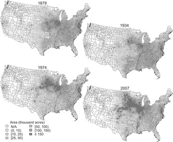
The footprint of U.S. corn area changed dramatically during the 13 decades beginning in 1879. At both the beginning and end of the period, the combined Corn Belt states of Indiana, Ohio, Illinois, Iowa, and Missouri accounted for a little less than one-half of overall U.S. corn acreage (45 percent in 1879 and 47 percent in 2007). While the relative importance of the Corn Belt remained more-or-less stable, there were dramatic shifts away from production in the Southeast and Appalachian regions and toward production in the Northern Plains and Lake States (for region definitions, see Appendix Figure 1 in the Online Appendix). In 1879, the Appalachian and Southeast regions accounted for about 27 percent of U.S. corn acres, but this share had decreased to just over 5 percent by 2007; over the same period, the Northern Plains and Lake States increased from a combined share of less than 10 percent of corn acreage to more than 38 percent.

Figure 1

U.S. CORN AREA, 1879–2007

Notes: The shading of each county indicates the number of harvested corn acres in that county (in thousands). Source: Created using data described in the text.

National acreage increased from 62 million acres in 1879 to 86 million acres in 2007, an increase of 24 million acres.Footnote ⁸ This represents the combined effect of a loss of over 12 million corn acres in the Southeast and Appalachian regions and a 25.5 million acre increase in the Northern Plains and Lake States, netting about half of the additional corn acres. Most of the remaining new acres are accounted for by a 12 million acre increase in the Corn Belt.

The 2007 census reported a dramatic 18 million acre increase in corn harvested area over that reported in the previous census (2002), accounting for three-quarters of the net increase in harvested acres since 1879. Between 2002 and 2007, all regions posted increased corn acreage, and there was a small shift away from production in the Corn Belt and Lake States. While the Corn Belt's share of production slightly decreased over this five-year period, the region saw a nearly seven million acre increase in corn area, accounting for almost 60 percent of that region's total increase in output since 1879. This dramatic change occurred in just one-half of a decade, underscoring the ability of farmers to quickly adapt to changing market and environmental conditions, rapidly changing the footprint of production in the process.

Between 1879 and 2007, national corn output increased by nearly 11 billion bushels, from 1.8 billion bushels in 1879 to 12.7 billion bushels in 2007. Production increased in all regions of the country, but the majority (89 percent) of the increased production was in the Corn Belt, Northern Plains, and Lake States. By contrast, the Southeast and Appalachian regions saw their share of national production decrease from more than 16 percent to under 4 percent. The Delta States maintained around a 3 percent share of national production, and now account for about the same amount of production as the Appalachian states.

County-level area data are plotted in Figure 1.Footnote ⁹ The county maps largely reflect the changes in regional production and area described earlier, but they also reveal significant intra-regional changes—the relative county area within each region did not remain constant. For example, additional area was not added to the Lake States and Northern Plains in proportion to the existing area—counties in the northern portions of these regions saw disproportionate increases relative to the other parts of the regions. Similarly, while the Southeast and Atlantic regions decreased their area, the counties near the Atlantic Coast actually increased their corn acreage.

One way to characterize the changing spatial footprint of corn production is to consider changes in the centroids of output and area. The centroid of a spatial variable, also referred to as the mean center, is the point that minimizes the sum of squared distances to all other points. In the present case, each bushel of corn or acre under corn production can be considered a point, so that the goal is to minimize the weighted sum of squared distances.Footnote ¹⁰ To simplify calculations it is assumed that all corn is grown at the geographic center of the county in which it is produced. So, for example, the centroid of output for a given year is the point on the map that minimizes the sum of squared distances from each county center to the point, with each distance weighted by the county production for the year—in essence, it represents the geographical pivot point of U.S. corn production.

To simplify calculations for this and later analysis, all points were projected onto a flat surface using the Albers Equal Area Conic projection formulae provided by John Snyder (Reference Snyder1987) and represented in meters east and north of a central point, thus allowing for use of Euclidian geometry to derive distances between points. This projection results in some minor distortions of distance (up to 1.25 percent for the conterminous United States), as Snyder (Reference Snyder1987, pp. 97–100) and the references therein discuss in more detail.Footnote ¹¹

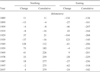
Over the 130 years for which complete county-level data are available, the mean center of corn output moved nearly 279 kilometers west and 157 kilometers north of the 1879 mean center, that is, from central Illinois to southeastern Iowa. The mean center of corn area has moved even more, shifting 343 kilometers to the west and 278 kilometers to the north. While the 2007 area and output mean centers are at about the same location in southern Iowa, the 1879 area centroid fell 78 kilometers to the east and 123 kilometers to the south of the production centroid. This implies that in 1879, areas north and west of the centroid were relatively higher-yielding than average, and that the movement of the centroid caused (or was caused by) expansion into relatively high-yielding areas.

As the present concern is with the relationship between area and output, we consider only data dating back to 1879 when both variables are available. However, Olmstead and Rhode (Reference Lange, Olmstead and Rhode2011) considered the distribution of U.S. corn area dating back to 1839, and showed that the pre-1879 shifts were rather large—there was substantial momentum in the crop's northwesterly movement before the period considered in the present study. Over the entire period 1839–2002, the crop's median location of production moved generally northwest, into cooler and drier areas.

The mean centers took a circuitous route from their 1879 locations to their 2007 locations. Table 1 summarizes movements in the mean center of area for nine- or ten-year periods ending in the indicated census years. The movements are described as period-to-period changes and as cumulative centroid movements to the east (easting) and to the north (northing), and negative values indicate movements in the opposite direction. The centroid moved to the west and north in most, but not all, periods. The two decades during and following the Dust Bowl (the period ending 1939) saw a substantial (but short-lived) easterly shift in the location of corn production followed by a large northerly movement during the subsequent decade. The pace of northerly movement has slowed in recent decades, but there is still a sustained westward push.

Table 1

MOVEMENT IN THE CORN MEAN CENTER, 1879–2007

Notes:

Each value represents the movement of the corn area mean center to the east (easting) or north (northing), relative to the previous centroid. The values for 1889 represent the movement from the 1879 mean centers.

Source:

Calculated using data described in the text.

Some of the movement is likely explained by shifts enabled by technological change, and shorter duration varieties in particular (see Olmstead and Rhode 2011), and consequent changes in relative regional productivity. Further, Geoff Cunfer (2005, pp. 88–89) notes that settlers often initially planted corn for livestock feed, but later planted other crops more suited to the local environment. This was especially pronounced in the Southern Plains, where farmers substituted sorghum for corn, and was exacerbated by the Dust Bowl, which induced a longer run shift away from corn in that region after 1935 (Cunfer 2005, p. 92). Crop substitution likely influenced the large pre-1879 shifts as well, for example increasing southern specialization in cotton after the Civil War (see Wright 1986, pp. 34–39).

Other factors such as settlement and urbanization patterns are also important, although the relationship between the changing population frontier and farming locations is rather complex (see Maizel et al. Reference Maizel, White, Root and Sisk1999 and Gardner Reference Gardner2002). Improvements in transportation and communication infrastructure also influenced the footprint of production, namely by allowing for regional specialization in the crops most suited to the local agroecological environment (Kim Reference Kim1998), thus, for example, allowing Iowa and Illinois producers to deemphasize livestock production, instead shipping corn to feed animals reared in other areas (Bogue Reference Bogue1963, pp. 12–13). The rapid expansion of the railroad networks in the decades around the turn of the twentieth century that helped enable such spatial specialization is particularly striking (see Atack Reference Crosby2013). In addition to development of transportation systems, Pamela Waisanen and Norman Bliss (Reference Waisanen and B. Bliss.2002) summarize a number of other factors that spurred a northwesterly movement in cropping generally, including development of tile drainage (e.g., allowing planting on wetlands in the upper Midwest), increased irrigation in the western states, and collapse of the sharecropping system in the south. Olmstead and Rhode (Reference Lange, Olmstead and Rhode2008, pp. 86–93) provide insight into the effect of various pests, diseases, and weeds on the relative suitability of different regions to growing corn.

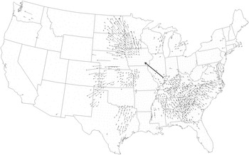
Figure 2 describes the relative contribution of each county to the movement of the national area centroid. The bold arrow shows the movement in the national centroid, with the origin point representing the 1879 national area centroid and the tip of the arrow representing the 2007 centroid.Footnote ¹² The area centroid moved northeast from southeastern Illinois to southeastern Iowa. Each of the smaller black arrows originates at the geographic center of a county, and longer arrows indicate that the county had a relatively large impact on the centroid movement; counties without arrows (represented by dots) did not have much effect on the movement of the national centroid.Footnote ¹³ The arrowheads indicate the direction in which the national centroid was pulled by the change in area in the corresponding counties.

Figure 2

CONTRIBUTIONS TO THE MOVEMENT OF THE AREA CENTROID, 1879–2007

Notes: The movement of the national area mean center of corn production is shown by the bold arrow. The amount by which each county affected the movement of the mean center is indicated by the length of the black arrow that starts at each county's centroid. The angle of each arrow represents the direction in which the area change in the county moved the national centroid. Counties that did not have much effect on the national mean center are represented by dots. See Footnote 13 for more details. Source: Derived using data described in the text.

The figure highlights a number of important trends. Although the Corn Belt exhibited an increase of 12 million acres over the entire period, changes in the spatial location of production within that region did not markedly affect the national centroid. This is at least partially because the centroid was already located in the Corn Belt, so the counties in that region had little torque in moving the centroid. Among the Lake States, a number of counties in southern and western Minnesota pulled the centroid markedly to the north, as did the eastern counties of the Dakotas. Changes in Texas largely cancelled each other, with increases in the counties on the Ogallala Aquifer (see Cunfer Reference Cunfer2005 and Hornbeck and Keskin Reference Hornbeck and Keskin2014 for discussions of the varied effects of tapping the Ogallala Aquifer) and offsetting decreases in the eastern portion of the state. Finally, reduced acreage shares in the counties of the Southeast and Appalachian states on net had a large impact on the centroid, almost uniformly moving it to the northwest.

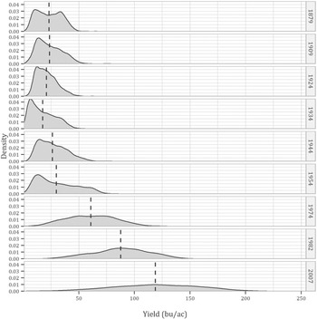
As implied by Figure 2, there have been substantial changes in the relative distribution of production and area across counties, however it remains unclear how the distribution of yields has changed over time. Figure 3 shows smoothed county-level yield densities for selected years. As expected, mean yields generally increase over time. However, neither (non-area weighted) mean nor median yields change appreciably from 1879 to 1924, although the distribution becomes increasingly positively skewed over this period (from a skewness value 0.17 in 1879 to 0.71 in 1924). The 1934 distribution is of particular interest since the represented year occurred during the Dust Bowl; as a result, both the mean and median yield decreased, and the coefficient of variation increased sharply, from about 0.44 in 1924 to 0.64 in 1934. The most pronounced effect was in the movement of the first yield quartile from 13.5 bushels per acre to 7.7 bushels per acre; the effect was less pronounced in the higher-yielding portion of the distribution such that the inter-quartile range was larger than the median by about 20 percent. As noted by Richard Sutch (Reference Robert, Nordhaus, Shaw, Libecap and Steckel2011, p. 214), “[w]hat the droughts starkly demonstrated was that the relative yield of hybrid corn was greatest when the absolute yields were generally depressed.” Indeed, the muted response of hybrid varieties to drought likely spurred their rapid adoption beginning in the latter part of the Dust Bowl. As a result of this rapid adoption, along with increased use of chemical fertilizers and other inputs, the years after the Dust Bowl saw steady increases in median and mean yields, and steadily decreasing spatial skewness—by 1982, the distribution became slightly negatively skewed, although the distributions were more-or-less symmetric starting in the 1960s when hybrid varieties were nearly completely adopted across the country (see Griliches Reference Griliches1960 and Dixon Reference Dixon1980).

Figure 3

DISTRIBUTION OF COUNTY CORN YIELDS, 1879–2007

Notes: The plots represent densities smoothed with a Gaussian kernel estimated using bandwidths determined by “Silverman's rule of thumb, ” namely, 1.06·min(s, IQR/1.34)·n –1/5, where 1.06 is the typical parameter used for Gaussian kernels, IQR is the interquartile range, and s is the sample standard deviation. The vertical dotted lines represent the (unweighted) mean county yield for that year. Source: Calculated using data described in the text.

There have long been a number of counties in the Corn Belt with relatively high production and yields. The two modes apparent in the 1879 distribution (Figure 3) appear to have resulted from low yields in the Southeast, Southern Plains, and Delta States (lower mode) contrasted with higher yields in the Corn Belt, Northern Plains, and Lake States. By 1974 a number of counties in the Northern Plains had surpassed the highest yields in the Corn Belt, although the Northern Plains also contained a number of counties with yields among the lowest nationwide. Over the subsequent three decades, the Corn Belt, Lake States, and Northern Plains saw marked increases in the yields of their largest-producing counties although, as in 1974, the Southern Plains had several moderately important high-yielding counties.

Moreover, the spatial distribution of yields has widened. In 1879, the average yield of the highest 5 percent of the yielding counties was 5.6 times greater than the yield of the lowest 5 percent of counties. By 2007, the difference had increased to 7.3 times. About on-fifth of the highest-yielding counties in 2007 entered production after 1879, while more than one-third of 1879's lowest-yielding counties stopped producing corn. Thus, some of the national yield increase is attributable to counties moving into and out of production.

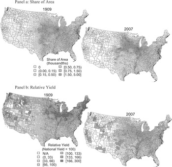
Figure 4 maps the national share of area accounted for by each corn producing county in 1909 and 2007 (Panel a). The share of area in the Corn Belt, Lake States, and Northern Plains counties has increased, at least partially due to relative decreases in the other parts of the country. The bottom maps (Panel b) show each county's yield relative to the national yield for each of the years (where national yield in each of the two years is set equal to 100). The changes in relative yield have been noticeably different from the relative area changes. The relative yields decreased, for example, in many of the counties that most markedly increased their acreage share, so that the Corn Belt now looks much more like the other major corn producing areas in terms of its yields.

Figure 4

RELATIVE YIELDS AND AREAS, 1909 AND 2007

Notes: The top figures show the share of national area accounted for by each county, in thousandths. The bottom figures show the yield of each county, relative to the national yield in the given year, which is indexed to be 100. Source: Calculated using data described in the text.

SPATIAL OUTPUT INDEXES—QUANTIFYING THE EFFECT OF LOCATION ON OUTPUT

The often confounding changes in relative yield, relative area, and in the total area devoted to corn make it difficult to understand exactly what has caused national output to change. This section develops a new, spatially-sensitive method for decomposing a change in national output into changes in national area, yield, and the relative county-specific areas under production.Footnote ¹⁴ As will be seen, comparatively simple concepts from economic index theory can be used, with slight modification, to decompose the national yield change. The analysis takes the yield changes as given, and would not be possible without having production and area data mapped to consistent county boundaries.

Spatial Output Indices

Let a_t and y_t represent vectors of county-specific corn acreages and yields for some year, t. The length of each vector is equal to the number of counties, and they are arranged such that the i ^th element of each vector corresponds to the same county (thus, a_it · y_it is the total output of county i in year t). Then, total production in year t is the sum y_t ′a_t , and the ratio of national output between year-t and some base year, b, is a simple index of output:

(1)

Multiplying the numerator and denominator by y_t ′a_b and rearranging terms reveals that:

(2)

where we define the first term as a Paasche area index (hereafter denoted I^P _A ), and the second term as a Laspeyres yield index (I^L _Y ).Footnote ¹⁵ A more convenient notation can therefore be employed:

(3)

By symmetry, the output index can also be decomposed into a Laspeyres area index and a Paasche yield index,Footnote ¹⁶ namely I^S _O = I^P _AI^L _Y = I^L _AI^P _Y , so that the output ratio can be defined by the product of a set of hypothetical quantities:

• • the output ratio that would result if the yield in each county were held constant at the year-t (year-b) value, allowing the area in each county to change, as represented by I^P _A (I^L _A ), and

• • the output ratio that would result if the area in each county were held constant at the year-b (year-t) value, allowing the county yield levels to change, as represented by I^L _Y (I^P _Y ).Footnote ¹⁷

Both specifications are equally valid, and which is appropriate for a given assessment depends on the questions to be answered.

The area indexes are of particular interest as they are well-suited to answer questions about the output consequences of changes in the spatial allocation. For example:

• • How much did the change in county areas contribute to current output (I^P _A )?

• • What would the change in production have been if the change in county areas had occurred in the base year (I^L _A )?

However, the area indexes are difficult to interpret—they confound the effects of changes in national area with changes in relative production. If, for example, all counties increased their harvested area by 25 percent between a base period and year-t, both area indexes would equal 1.25 for time t (irrespective of any changes in yield). Alternatively, if harvested area were reallocated to counties with higher yield, with the total area under production and the yield vector are held constant, the resulting increase in production would also be reflected exclusively in the area indexes (even though national average yield would have increased). It would be useful to separate the scaling effect of a change in overall (national) area from the effect of spatially reallocating production.

For a general change in the area vector, I^L _A will always differ by I^L _A − A_t / A_b relative to its value under an equi-proportional area change of the same total magnitude (see the Online Appendix). If the index value is larger than A_t / A_b , the change in relative area shares (the footprint of agriculture) caused the index to increase. Therefore, the effect of the relative spatial reallocation can be summarized by:

(4)

The latter form suggests an index of the effect of the relative spatial reallocation, the Laspeyres version of which is:

(5)

Notice that this is equivalent to scaling each of the year-t areas in the numerator so that they sum to A_b , thus maintaining the relative year-t spatial allocation while removing the effect of the change in overall area. A similar Paasche-type reallocation index can be defined by scaling the year-b areas so that they sum to A_t :

(6)

The relative spatial reallocation indexes answer slightly different questions from those addressed by the area indices, namely:

• • I^P _R gives the amount by which output increased due to the change in the relative spatial allocation of corn area between the base year and year t, evaluated at year-t yields, and

• • I^L _R gives the amount by which output increased due to the change in the relative spatial allocation of corn area, evaluated at base-year yields.

The county production and area data do not include observations for all county-years in the panel, either because data were withheld due to privacy concerns or because there was no production in the given county-year (and in some census years, the reason for the null observations was not reported). In the latter case, the null values for area and production can be replaced with zeros. When data were withheld to maintain the privacy of individual producers, it is assumed that the production in the county-year was accounted for by just one or a few farms, and therefore that the total production and area in the county were not very large. The area and production in these cases are also assumed to be zero; in the majority of such cases the effect on the calculated index will be minor.

Missing yield observations are somewhat more problematic. Consider, for example, calculation of an area index. It is possible that a county with no reported production in, say, 1889, markedly increased its area and output by 2007. A Laspeyres area index that uses 1889 as its base year will have in its numerator the inner product of the base-year yields and the year-2007 areas. If some of the 2007 counties had no yield observation in 1889, using zero as the yield value will introduce a downward bias into the index. Had the crop been grown in the county in 1889, it is likely that the yield would have been positive, especially given that it was grown there in 2007 (otherwise the county would not affect the numerator of the index). To reduce the bias, it is helpful to estimate the yield that the county would have exhibited had it grown the crop, a notional “counterfactual yield.” To resolve this issue, the inverse-distance weighted mean of the county's three nearest neighbors for which production and area were reported is used as an estimate of the county's counterfactual yield in the period.Footnote ¹⁸

The Paasche and Laspeyres values for a given variable will not, in general, be the same, and the differences between the indexes have received more attention in the literature than most topics of similar importance. The inequality of the indexes is almost universally viewed as a deficiency among those whose goal is to determine, say, the rate of inflation or the growth in aggregate output, and many solutions have been put forth. These objections usually arise because it is rarely obvious whether one should choose the base period or the current period to weight the index, and many of the proposed solutions are constructed to take account of both weighting vectors. The Fisher index, for example, is calculated as the geometric mean of the Laspeyres and Paasche indexes for a given variable,Footnote ¹⁹ while the Marshall-Edgeworth index uses an arithmetic average of the weights. As shall be demonstrated, the basic spatial output indexes developed here will yield different information about the nature of production, and additional insight will be gleaned from the differences in the indexes—for the current purpose, it will be advantageous to keep the traditional weights and no attempt will be made to empirically reconcile disparities among the indexes.

Other formulations, such as the Young index (Young Reference Young1812) use expenditure shares from a given period to weight prices; if applied to the present problem this approach would be equivalent to holding the production shares of the counties constant at their base-period values. Holding total area constant while allowing the shares to change has no known analogue in the economic index domain, likely because neither the sum of prices nor that of quantities of different goods would have a readily interpretable meaning, while the sum of areas does.

Results

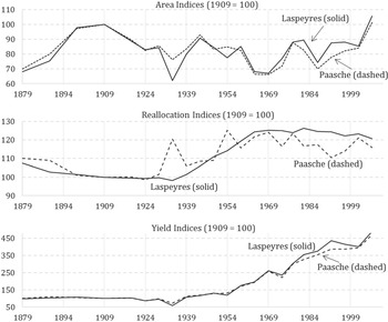
Figure 5 plots the calculated indexes, the values of which are provided in Appendix Table 1 in the Online Appendix. The solid lines in each panel represent Laspeyres indexes and the dashed lines represent Paasche indexes. The base year 1909 was chosen for all of the indexes because more counties were represented in 1909 than in the earlier years, thus minimizing bias that might result from the counterfactual yield estimation procedure described above.Footnote ²⁰ Before the base year, the area indexes (Figure 5, top panel) were generally increasing, as total area under corn production reached a peak in 1909. Over the same period, the yield indexes (Figure 5, bottom panel) both rose slightly then fell; both showed a net decrease by 1909, indicating that yields were falling in both the new areas (I^P _Y ) and the old areas (I^L _Y ). This trend is reflected very clearly in the reallocation indexes (Figure 5, center panel)—which reveal the extent of change in U.S. corn output attributable to the change in relative area from the 1909 footprint of corn production, evaluated at the base-year yields (Laspeyres) or the current-year yields (Paasche)—and both show a fairly substantial and steady decrease between 1879 and 1909.

Figure 5

AREA, REALLOCATION AND YIELD INDEXES, 1879–2007

Notes: Please note the differing scales in the various panels, which caused the plotted versions of the yield indexes to appear smoother than the others; the coefficient of variation of the yield indexes is actually much larger than either the area or the reallocation indexes. See Appendix Table 1 in the Online Appendix for the values. Source: Calculated using data described in the text.

After 1909, the area indexes both fell, reaching troughs in the Dust Bowl year 1934.Footnote ²¹ Much of the decrease can be explained by a decrease in total area under production (I^S _A ). With such a sharp change in area, the reallocation indexes become particularly useful. In that year, a marked difference can be seen between the Laspeyres reallocation index value (98) and the value of the Paasche version (120). Thus, the “new” acres were less affected than the old acres, likely because production had already partially adjusted by 1934 (about four years into the Dust Bowl). Indeed, between 1929 and 1934, the Northern Plains reduced its corn acreage by more than 16 million acres (91 percent) and the region's average yield dropped by nearly 67 percent. The figures here use harvested acres, not planted area as the denominator for yield calculations. Thus, the present calculations do not capture the effect of crop failures (areas with zero yield) on the reallocation indices; the extent to which this biases the results depends on when and on which acres crop failures occur. Insofar as failures are more likely to occur on relatively low-yielding acres and in earlier periods, the reallocation indices will be biased downward and therefore tend to be conservative in attributing output increases to spatial reallocation.Footnote ²²

The Paasche reallocation index peaked sharply again in 1954, reaching a value of 125. As in the Dust Bowl, this was due to deleterious events that did not affect some of the highest-yielding areas: a heat wave covering the plains states, southern portions of the Corn Belt, and the southeast. The harvested corn acreage of Missouri fell by nearly one-quarter, while that of Kansas fell by more than 40 percent. Regarding Missouri, Nancy Westcott and Kevin Grady (Reference Westcott and Grady2010) report that “[t]he damage to the corn was particularly devastating as hot, dry conditions continued through the crucial tasseling stage…(p. 4).” However, the writers of the 1954 Agricultural Census note that the effect of the heat wave on the national yield was muted because of “…favorable weather conditions in most parts of the important corn producing States, the use of fertilizer and hybrid seed, and the improvement in tillage (Vol. 2, Part 7, p 580).” This story supports the divergence in the Paasche and Laspeyres reallocation indexes, and highlights the utility of tracking the indexes separately rather than trying to reconcile their differences.

So overall, how much of the change in U.S. corn output can be attributed to shifts in the location of production? Between 1909 and 2007, the change in the relative spatial allocation of production accounted for about 16 percent of the change in output according to the Paasche version of the reallocation index, and 21 percent according to the Laspeyres version (Figure 5, center panel). The shift in the location of production was enabled by (and in turn had effects on) a whole host of important production and productivity related factors. For example, changes in infrastructure affected the cost of market access (of both inputs and outputs) in different ways in different locations; changes in corn genetics changed the spatial comparative advantages of particular varieties in particular locales—most notably, the introduction of shorter duration varieties facilitated a movement of the crop into higher latitudes with shorter growing seasons, but with generally better water-buffered soils (allowing for higher planting densities), and lower pest and disease pressures. Changes in the genetics of other crops changed the relative local comparative advantages of growing cotton versus corn (say, in the Southern Plains) or wheat versus corn (say, in the Northern Plains and Lake States). Thus the change in corn output attributable to the spatial relocation of production is a mutatis mutandis attribution with respect to the spatial pattern of technology adoption, with a multitude of factors both enabling and being affected by these spatial shifts. That is, technological change over time for the national aggregate is controlled for by anchoring the assessment of the relocation effect by the use of base year (Laspeyres) or current year (Paasche) yields so that only the spatially variable aspects of changes in technology are embedded within the reallocation index.

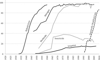
Notably, most of the increase in output attributable, mutatis mutandis, to relocating production occurred during the period of rapid hybrid and fertilizer adoption beginning in the 1930s through to the early 1960s period (see Figure 6), although previous technologies such as the corn belt dents enabled some of the earlier movement (Olmstead and Rhode Reference Robert, Nordhaus, Shaw, Olmstead and Rhode2008, p. 84). The share of U.S. corn acreage sown to hybrid varieties increased from less than 1 percent in 1933 to more than 95 percent by 1960; less than one-half the U.S. corn acreage was receiving any chemical nitrogen fertilizer in 1950, by 1966 more than 90 percent was being fertilized (and the average application rate increased markedly as well, from 5.1 pounds per acre of active ingredient in 1950 to 59.1 pounds per acre in 1966).

Figure 6

CORN TECHNOLOGY ADOPTION

Notes: The variables represent the percentage of harvested corn acres on which the technology was adopted in each year. Source: Data for nitrogen use on corn acres for 1947–1959 are from Ibach and Adams (1967), except for 1950 which is from Mehring, Adams, and Jacob (1957) and 1959 which is from Ibach, Adams, and Fox (1964). Nitrogen use data for 1964–2005 are from USDA-ERS (2011). Herbicide data for 1952 and 1958 are from Eichers, Andrilenas, and Anderson (1978) and values for 1993–2005 are from USDA-NASS (2011a). All other herbicide use data are from Lin et al. (1995). Irrigation data for 1969–1994 are from USDA-ERS (1994) and data for 1997–2007 are from USDA-NASS (2011b). Insecticide use data for 1952 and 1958 are from Eichers, Andrilenas, and Anderson (1978) and from Lin et al. (1995) for other years. See Alston et al. (2010, p. 253) for information on hybrid maize and genetically modified maize adoption.

The footprint of production is also influenced by policy. Roger Claassen, Andrea Cattaneo, and Robert Johansson (Reference Claassen, Cattaneo and Johansson2008) describe three waves of policy-induced land idling, largely spawned by the Agricultural Adjustment Act of 1936, the Soil Bank and the Conservation Reserve Program (CRP). The effect of land idling on the reallocation indices depends on which acres tend to be relatively more affected by the programs. Patrick Sullivan et al. (Reference Sullivan, Hellerstein and Hansen2004) found that only about one-half of the land enrolled in the CRP would return to cropping if the program were to expire, which implies that the CRP tends to idle relatively less productive land. However, the net effect of idling programs on the reallocation indices is not clear as so-called “slippage” causes generally less productive land to be brought into production (see Wu Reference Wu2000) and there is strong evidence that such programs incentivize production on marginal land (Sylvester et al. Reference Sylvester, Brown and Deane2013, p. 13). Further, Sullivan et al. (Reference Sullivan, Hellerstein and Hansen2004) find that the effect of the program is not uniform, with the Southwestern Corn Belt and Northern Plains setting aside more area than other regions, implying that policy may be muting the potential output gains from spatial reallocation.

The corollary to the observation that the major output consequences of moving the location of corn production occurred during the 1930–1960 period is that spatial reallocation effects contributed little to the overall growth in national output during the subsequent four decades for which we have data—both reallocation indexes were more-or-less constant during the 1960s and 1970s, and generally decreased slightly thereafter. Across the board growth in corn yields was the main reason that corn output roughly doubled during the 1960 and 1970 period.Footnote ²³ Particularly noteworthy is the marked increase in national yield and area reported in the 2007 census over that reported in the 2002 census.

Beginning in 1959, the Laspeyres reallocation index is always higher than the Paasche reallocation index. This occurred because yields grew somewhat slower on average in counties that increased their share of national area, such that the average relative yield advantage of those areas, while still positive, was lower than it was in the base year.