I. INTRODUCTION
A. Background
The main mission of the National Institute of Standards and Technology (NIST) is to promote U.S. innovation and industrial competitiveness by advancing measurement science, standards, and technology in ways that enhance economic security and improve the quality of life. Activities associated with the mission of advancing the standards and measurements include those which
(i) develop, maintain, and retain U.S. primary standards for the structure and properties of materials and provide the means and methods for making measurements consistent with those standards, for example, develop and distribute reference materials
(ii) contribute to the development of technically sound standard test methods by participating in national and international standards developing organizations
(iii) and provide critically evaluated materials data to customers.
The efficiency of thermoelectric energy conversion or cooling is related to the dimensionless figure of merit (ZT) of a thermoelectric material,Reference Tritt and Subramanian1, Reference Tritt2 given by ZT = S2σT/k, where T is the absolute temperature, S is the Seebeck coefficient, σ is the electrical conductivity, and k is the total thermal conductivity. ZT is directly related to the coefficient of performance of a thermoelectric material and is the principal criterion by which these materials are judged. Low conversion efficiency has restricted the commercial use to only small-scale devices. Thermoelectric materials with desirable properties (ZT > 1, i.e., characterized by high electrical conductivity, high Seebeck coefficient, and low thermal conductivity) could have widespread military and industrial applications. In recent years, relatively high ZT values have been found in both thin films and bulk materials.Reference Hsu, Loo, Guo, Chen, Dyck, Uher, Hogan, Polychroniadis and Kanatzidis3–Reference Rao, Ji and Tritt6 Continued efforts to identify novel materials and optimize existing materials are crucial for large-scale applications. Most importantly, the accuracy and precision of reported high ZT measurements must be confirmed.
Characterization of thermoelectric materials is performed through measurements of the electrical resistivity/conductivity, the thermal conductivity, and the Seebeck coefficient. These measurements are often demanding; however, one of the most important initial measurements is that of the Seebeck coefficient. Measurement of only the Seebeck coefficient can filter out those materials that do not have the desired thermoelectric properties.
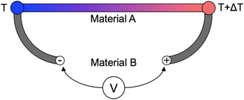
The Seebeck effect, illustrated in Fig. 1, is the direct conversion of a temperature gradient, ΔT, maintained between the two interfaces formed of two dissimilar conductors A and B, into an electric potential, V, (in the presentation of results later, this is called ΔV). The voltage produced is directly proportional to the temperature gradient, and the proportionality constant, SAB, is defined as the Seebeck coefficient:

Schematic of the Seebeck Effect.

The Seebeck coefficient is equal to the difference in the Seebeck coefficients of the two materials:

Thus, if one knows the Seebeck coefficient of one of the materials in the loop, the Seebeck coefficient of an unknown material can be determined.
Measurement apparatus for the Seebeck coefficient include both commercial and custom-built systems. Although data from different systems are commonly compared, there is no Seebeck coefficient SRM for either the low (≤400 K) or the high temperature (≥400 K) regime. A Seebeck coefficient SRM would provide measurement reliability and interlaboratory comparison capabilities. Furthermore, a higher level of certainty in the value of Seebeck coefficient will lead to greater certainty in the value of ZT. The low-temperature Seebeck coefficient is important for potential electronic refrigeration applications, whereas the high-temperature Seebeck coefficient is important for power-generation applications. As a first step, we have completed the development of a Seebeck coefficient SRM for the low-temperature regime (10 K–390 K). The temperature range that is covered by this low-temperature SRM offers some crossover with the temperature range of the high-temperature equipment as well. Therefore, this low-temperature Seebeck coefficient SRM will provide a full calibration for low-temperature measurement equipment and a partial calibration for high-temperature measurement equipment.
B. Requirements for the Seebeck coefficient SRM
A number of aspects had to be considered when developing the Seebeck coefficient SRM.7 First, the material should possess long-term stability. In addition, the material should be homogeneous and producible in a large consistent batch. A large homogeneous batch would allow for measurements of representative samples to provide data indicative of the entire batch. Second, the SRM had to be certified over a broad temperature range as most researchers in this field perform temperature-dependent measurements. Measurements are usually divided into the low-temperature regime (≤400 K) and high-temperature regime (≥400 K). Although there is normally some overlap between these regimes, they typically require different measurement equipment. Third, it is important that the SRM possesses a Seebeck coefficient with a magnitude on the order of that typically measured in the field. This value should be near the middle of the range of 25–400 μV/K. Fourth, the SRM should be available at a reasonable price to the community; therefore, the development and production must be cost-effective. Fifth, as we consider development of the SRM, considerations must be given to future SRMs. It might be possible to use the same material for future thermoelectric related SRMs. These could be produced for other physical properties, for ZT, or for other sample geometries such as thin films.
C. Previous round-robin measurement survey
Prior to the certification process, we completed a measurement survey to determine the feasibility of producing the SRM, the measurement consistency of the candidate materials, and the best measurement technique for providing the standard data.Reference Lowhorn, Wong-Ng, Lu, Zhang, Thomas, Otani, Green, Tran, Caylor, Dilley, Downey, Edwards, Elsner, Ghamaty, Hogan, Jie, Li, Martin, Nolas, Obara, Sharp, Venkatasubramanian, Willigan, Yang and Tritt8, Reference Lu, Lowhorn, Wong-Ng, Zhang, Thomas, Otani, Green, Tran, Caylor, Dilley, Downey, Edwards, Elsner, Ghamaty, Hogan, Jie, Li, Martin, Nolas, Obara, Sharp, Venkatasubramanian, Willigan, Yang and Tritt9 Two candidate materials were chosen. Constantan is well known as a simple alloy (55 at.% Cu/45 at.% Ni), commonly used in thermocouples with a moderate Seebeck coefficient at room temperature. Cylindrical samples (6.47 mm long by 3.45 mm diameter) were purchased from Concept Alloys (Whitmore Lake, MI). Bi2Te3 is a state of the art thermoelectric material with a high Seebeck coefficient at room temperature. Samples with no intentionally added dopants were obtained from Marlow Industries (Dallas, TX) in a rectangular shape (approximately 6.08 mm long by 3.04 mm2).
Measurements were performed in two rounds by 12 international laboratories involved in active thermoelectric research using a number of different commercial and custom-built measurement systems and techniques. The detailed statistical analyses on the interlaboratory measurement results and the statistical methodology for analysis of irregularly sampled measurement curves in the interlaboratory study setting have been reported earlier.Reference Lowhorn, Wong-Ng, Lu, Zhang, Thomas, Otani, Green, Tran, Caylor, Dilley, Downey, Edwards, Elsner, Ghamaty, Hogan, Jie, Li, Martin, Nolas, Obara, Sharp, Venkatasubramanian, Willigan, Yang and Tritt8, Reference Lu, Lowhorn, Wong-Ng, Zhang, Thomas, Otani, Green, Tran, Caylor, Dilley, Downey, Edwards, Elsner, Ghamaty, Hogan, Jie, Li, Martin, Nolas, Obara, Sharp, Venkatasubramanian, Willigan, Yang and Tritt9. On the basis of these results, we have selected Bi2Te3 as the SRM (designated as SRM 3451).
II. DESCRIPTION OF THE SEEBECK COEFFICIENT SRM
SRM 3451 is entitled “Low-Temperature Seebeck Coefficient Standard (10 - 390 K)” and provides members of the thermoelectric materials community the means to calibrate Seebeck coefficient measurement equipment (for bulk materials), in the stated temperature range.
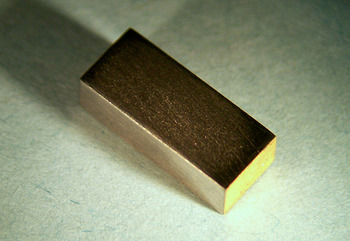
The SRM artifact, shown in Fig. 2, is a bar-shaped piece of nonstoichiometric bismuth telluride (n-type, Te rich, Bi/Te ratio approximately 2/3, formula Bi2Te3+x; see, for example, Ref. Reference Scherrer, Scherrer and Rowe10). The SRM artifacts were custom prepared (involving ingot solidification, cutting and polishing of the bar-shaped pieces, and metal plating of their ends) for NIST by Marlow Industries. No modifications were made at NIST to the as-received SRM artifacts. The SRM artifact dimensions are approximately 3.5 mm × 2.5 mm × 8.0 mm.
Photograph of the SRM 3451 artifact.

Marlow Industries carefully weigh the Bi and Te for ingot preparation to achieve x = 0.004 ± 0.002. The correct composition range is verified by comparing the measured electrical resistivity of the ingot to previous composition/resistivity calibrations. According to Marlow Industries, this optimal resistivity value at room temperature is 1.2 ± 0.1 mΩ-cm. To facilitate good electrical contact between the SRM artifact and the leads to be attached to it, Marlow Industries deposited a 2–3-μm-thick nickel (Ni)/100-nm-thick gold (Au) bilayer on both ends of the artifact, using a standard process.Reference Sankara Narayanan, Baskaran, Krishnaveni and Parthiban11, Reference Das, Limaye, Grover and Suri12 The outer Au layer creates a wettable surface for soldering external leads to the artifact; the inner Ni layer acts as a diffusion barrier between the Au/solder and the bismuth telluride.Reference Tritt and Rowe13
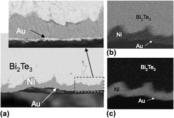
Figure 3 contains three scanning electron micrographs of a typical SRM 3451 artifact, showing the interfaces between the Au, Ni, and bismuth telluride. X-ray energy-dispersive spectroscopy analysis of the SRM was conducted. Figures 3(b) and 3(c) show no observable interactions at the bismuth telluride/Ni and Ni/Au interfaces. Diffusion of Au and Ni into each other and into bismuth telluride is not significant at the Au and Ni deposition temperatures (<100 °C).Reference Tritt and Rowe13 Nonetheless, the Seebeck coefficient measured on the artifact, which comprises the Au/Ni/bismuth telluride/Ni/Au bar, would incorporate the effect of any insignificantly small amount of impurity diffusion; moreover, since all the artifacts are from the same lot and were similarly processed, the effect would be the same for all pieces.
(a) Scanning electron micrograph (backscattered electron image) of a polished cross section of a typical SRM 3451 artifact, showing the interface between the Au (light), Ni (gray), and bismuth telluride (also light) regions; x-ray energy-dispersive spectroscopy maps of the Standard Reference Material (SRM) showing (b) Te Lα distribution and (c) Ni Lα distribution.

III. SRM MEASUREMENT AND ANALYSIS
A. Measurement technique
Certification measurements were obtained using a differential steady-state (DC) technique. Additional reference measurements were obtained using a transient (AC) technique. In this section, we discuss only the DC technique; the SRM certification data are based only on the DC measurements.
Ten artifacts were selected randomly from the batch of 390 received from Marlow Industries, and numbered SRM01 to SRM10. Using the DC technique, five of these artifacts were measured once. The remaining five artifacts were measured twice: for the second measurement, the contact leads were removed and reattached on the opposite ends of the artifacts. Thus, a total of 15 datasets were obtained. In addition, all 10 artifacts were measured once using the AC technique (see Sec. V for these data).
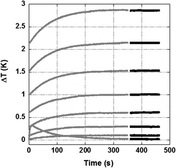
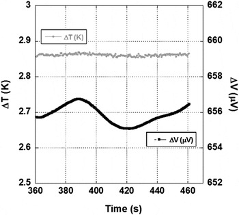
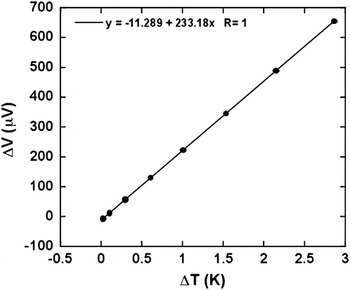
The measurements were performed under a vacuum of <10−5 Pa. During the measurements, each artifact was maintained at a constant base temperature while a range of ΔT values (where ΔT ≤ 0.01T) were applied, and the corresponding ΔV values were measured. For each ΔT, the artifact was stabilized for a period ranging from 25 to 400 s, depending on the temperature. The corresponding ΔT and ΔV measurements were then made over an additional time period of 25–100 s and averaged over that period. Figure 4 shows ΔT as a function of time for eight different ΔT values during the stabilization (gray) and measurement (black) periods. Typical ΔT and ΔV fluctuations during a measurement period are shown in Fig. 5. The time-averaged values of ΔV were plotted as a function of the corresponding ΔT for each base temperature; the Seebeck coefficient was derived from the linear fit of these data, as shown in Fig. 6 for a base temperature of 300 K. This method of fitting the data obtained from multiple (ΔT, ΔV) measurements avoids the assumption that any given data point and the origin (ΔV = 0, ΔT = 0) are collinear, thus effectively eliminating any offset voltage.
ΔT as a function of time for eight different ΔT values during the stabilization (gray) and measurement (black) periods. For each ΔT, the artifact was stabilized for a period ranging from 25 to 400 s. Corresponding ΔT and ΔV measurements were then made over an additional time period of 25–100 s and averaged over that period. These data are from SRM01 at 300 K base temperature.

Typical data showing ΔT and ΔV during the measurement period. The x-axis starts at 360 s (after the stabilization period). These data are from SRM01 at 300 K base temperature and a ΔT of 2.86 K.

Plot of time-averaged values of ΔV and ΔT. These data are from SRM01 at 300 K base temperature. The slope is the Seebeck coefficient at this temperature.

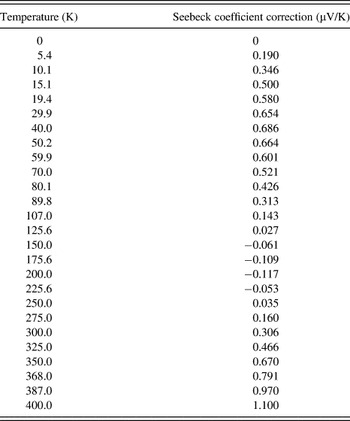
Finally, each measured Seebeck coefficient value was corrected for the Seebeck coefficient of the lead wires attached to the artifact (made of manganin, a well known alloy of 86 at.% copper, 12 at.% manganese, and 2 at.% nickel), according to Eq. (2), using the interpolated manganin S values listed in Table I.
Seebeck coefficient values for manganin lead wires.

B. Measurement hardware and software
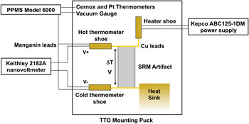
The measurements were performed on a Quantum Design Physical Property Measurement System (PPMS; Model PPMS-9, San Diego, CA).14 Two third-party instruments were interfaced with the system: a Keithley 2182A nanovoltmeter (Keithley Instruments, Inc., Cleveland, OH) used to measure ΔV and a Kepco ABC125DM power supply (Kepco, Inc., Flushing, NY) to generate the heater current for creating the ΔT. A schematic of the measurement system is shown in Fig. 7.
Schematic depicting artifact mounting for Seebeck coefficient measurement.

The artifacts were mounted with a dual-probe configuration, shown schematically in Fig. 7. A disk-shaped copper contact lead was soldered to each end of the artifact. These contact leads had a circular middle section with two thin extensions for attaching the thermometer (Cernox 1050, Quantum Design, San Diego, CA) and heater (resistive chip heater). The artifact and attached leads were mounted on the Quantum Design Thermal Transport Option (TTO) puck. One side of the bottom lead was screwed into the heat sink. The cold thermometer shoe was screwed onto the other side of the bottom lead. The heater shoe was screwed onto the bent side of the top lead, while the hot thermometer shoe was screwed onto the opposite side. The hot and cold thermometer shoes also acted as electrical probes for measuring ΔV along the artifact.
The hot and cold thermometers were calibrated prior to starting the certification measurements, using the Quantum Design calibration procedure with the TTO calibration fixture assembly (P/N 4084-595). In this procedure, the thermometers are mounted to a gold-plated copper calibration sample provided with the TTO system, which acts as a thermal short between the system thermometer and the hot and cold thermometers. Helium gas in the measurement chamber and the thermal short allow the three thermometers to be at the same temperature. The system thermometer is calibrated to a NIST-traceable primary Cernox thermometer for temperatures <100 K and a NIST-traceable platinum thermometer for temperatures >100 K. The resistance of the hot and cold thermometers is measured as a function of the system temperature to generate a resistance–temperature calibration curve.
Custom software was written using National Instruments LabVIEW (National Instruments Corporation, Austin, TX) to automate measurements and data collection.
C. Seebeck coefficient measurements
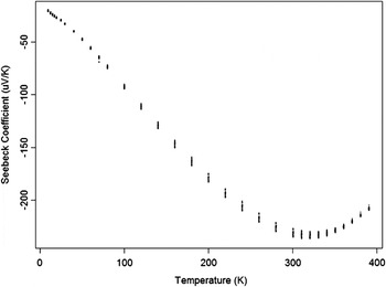
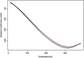
The Seebeck coefficient is derived by plotting the measured electric potential, ΔV, as a function of the measured temperature difference, ΔT, as shown in Fig. 6. To determine the Seebeck coefficient as a function of temperature, such measurements were carried out at 32 different base temperatures. Figure 8 displays the temperature dependence of the Seebeck coefficient; this plot contains 15 datasets measured on 10 different artifacts (since, as described earlier, 5 of the 10 artifacts were measured twice).
Seebeck coefficient as a function of base temperature (15 datasets).

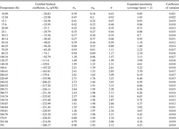
The mean Seebeck coefficient (Sm) was then computed at each base temperature, and the means are listed in the second column of Table II.
Certified Seebeck coefficient values for SRM 3451.

D. Parameterization of the Seebeck coefficient data
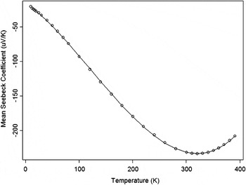
The mean Seebeck coefficient data (Table II) have been parameterized as a Taylor expansion around T = 200 K:

where the parameters a 0,a 1,a 2,a 3, and a 4 are determined to be −25.02319, −0.7739003, 0.001841421, 7.723781 × 10⁻⁶, and −1.065563 × 10⁻⁹, respectively.
This equation serves as an interpolation model for obtaining Seebeck coefficient values at temperatures in between the 32 measured values. The model is purely empirical, and the parameters have neither physical meaning nor units. Figure 9 shows the excellent fit to the data.
Mean (symbols) and parameterized (curve) Seebeck coefficient data as a function of base temperature.

E. Seebeck coefficient uncertainty analysis
Uncertainty analysis was conducted in accordance with the procedures and policies outlined in NIST Technical Note No. 1297.Reference Taylor and Kuyatt15 Uncertainties associated with the results of the Seebeck coefficient measurements may be categorized as either type A or type B, defined classically as those uncertainties that can be evaluated statistically (A) or those that cannot (B). Type A components must be characterized by a statistically analyzed series of observations, while type B components may be systematic in origin. The final standard uncertainty is the combined uncertainty of type A and type B uncertainties.
In our analysis, we assume that all contacts are Ohmic and that all lead wires (including solder interfaces) are appropriately connected such that the law of intermediate metals applies.Reference Burns and Scroger16 Therefore, any temperature-independent voltage or thermal offset between the contact and the “measurement location” is effectively eliminated by linearly fitting the ΔV and ΔT data. Any nonsystematic offsets are best treated statistically based on our combined series of measurements.
1. Type A uncertainties
The type A uncertainty, σA, consists of two components, σA 1 and σA2. σA 1 is the average standard deviation derived from identical measurements on 10 different artifacts and, therefore, contains sample to sample variations. σA2 is the average standard deviation on two measurements made on each of five of the artifacts (second measurement with leads reversed) and, therefore, reflects variations in the artifact-mounting technique.
The type A standard uncertainty is given by:

σA values are tabulated in Table II as a function of temperature.
2. Type B uncertainties
Type B uncertainties are systematic in origin and primarily derive from instrumentation, data acquisition, and/or calibration errors. Therefore, only those systematic uncertainties arising from the measurement of the hot and cold temperatures and the electric potential are considered.
We must consider the uncertainty contributions from both the hot and the cold thermometer measurements. According to the calibration procedure described in Sec. III. B and vendor design specifications, the standard measurement uncertainty for each thermometer is 0.6% T, for any T within the measurement range. Since ΔT is calculated as the difference between the hot and the cold temperatures, ΔT has an uncertainty of (0.62 + 0.62)1/2% = 0.85%. Consequently, the Seebeck coefficient, computed as the least square estimate of the slope based on the data {(ΔTi,ΔVi)} (see Fig. 6, for example), at each temperature point T, has the same 0.85% uncertainty.Reference Fuller17, Reference Berkson18 This uncertainty component, denoted σB 1, is given by:

Furthermore, there is an uncertainty associated with the measurement of the average sample temperature, T, given by the compound average of the collection of sample temperature values obtained for each ΔT and ΔV pair, where each sample temperature is calculated as the simple average using the hot and cold thermometer measurements. The uncertainty for the average of two temperatures can be computed easily in terms of uncertainties for individual temperatures, that is, [(0.6/2)Reference Tritt2 + (0.6/2)Reference Tritt2]1/2 % = 0.42%. To derive the Seebeck coefficient uncertainty component for the average base temperature, denoted σB 2, the Seebeck coefficient data were parameterized [Eq. (3)], and the derivative of the Seebeck coefficient data, S’m(T), was determined. The Seebeck coefficient uncertainty associated with the average base temperature uncertainty is given as:

We now turn to type B errors associated with the electric potential measurements. The manufacturer’s stated uncertainty for the Keithley 2182A nanovoltmeter is ± (50 × 10−6 of the voltage reading, plus 4 × 10⁻⁶ of the voltage range) at 1 year postcalibration. A typical uncertainty calculation is as follows: we take the largest ΔV that corresponds to the largest ΔT as a representative voltage from the collection of ΔV–ΔT pairs at the base temperature of 300.73 K. Using the Seebeck coefficient from Table II (231.36 μV/K) and the largest ΔT (2.86 K, see Fig. 6), we can calculate the thermoelectric voltage as (231.36 μV/K) × 2.86 K = 6.62 × 10⁻⁴ V. We are justified in using the average Seebeck coefficient for this estimation since the linear relationship between ΔV and ΔT in Fig. 6 is strong (R2 = 1). The voltage reading uncertainty is then calculated as (50 × 10−6) × (6.62 × 10−4 V) = 3.31 × 10⁻⁸ V. The voltage range uncertainty in the 10 × 10−3 V range (the range used in our certified measurements) is (4 × 10−6) × (10 × 10−3 V) = 4.0 × 10⁻⁸ V. Therefore, the total measurement uncertainty is ± (3.31 × 10⁻⁸ V + 4.0 × 10⁻⁸ V), resulting in a percent uncertainty for our representative thermoelectric voltage of (7.31 × 10⁻⁸ V)/(6.62 × 10−4 V) × 100 ≈ 0.01%.
Comparing the type B electric potential measurement uncertainty (≈0.01%) with the type B temperature measurement uncertainty (0.85%), it is clear that the contribution from the voltage measurement is about two orders of magnitude smaller and can be neglected.
Thus, the total type B uncertainty can be determined by combining the two temperature measurement uncertainty components:

σB uncertainty values are listed in Table II.
3. Total uncertainty
The total Seebeck coefficient measurement uncertainty is given by:

σ values are listed in Table II. Also listed in Table II are the expanded uncertainties (cσ, with coverage factor c = 2), and the coefficients of variation, which show that the certified Seebeck coefficients have a relative uncertainty of about 1–2%.
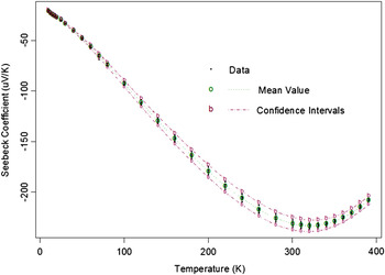
The certified Seebeck coefficient measurement data, along with the mean values and the confidence (uncertainty) intervals (Sm ± cσ, the 95% confidence intervals under the normal distribution assumption), are plotted in Fig. 10. All dotted lines are guides for the eye. The Seebeck coefficient uncertainty for any interpolated temperature value [using Eq. (3)] is given approximately by the σ value at a nearby measured temperature value (Table II). This is a typical approach when only discrete data are available.
Plot of certified Seebeck coefficient data with 95% confidence band. Dotted lines are guides for the eye.

IV. USE OF SRM
SRM 3451 is used for the calibration of instruments that measure low-temperature Seebeck coefficients (10 K to about 400 K). The SRM artifacts were packaged by the SRM Office and placed inside a plastic vial (one per vial) with screwed lid and gasket, under an inert atmosphere of argon gas. The sealed vial was then placed inside a heat-sealed mylar bag to keep out moisture.
Seebeck measurements should be performed by mounting the artifact in a manner as close as possible to that described in this document. We suggest that artifacts be mounted in a two-probe arrangement, with one probe connected to each end of the artifact with solder. These probes should also allow attachment of both a thermometer and a voltage probe. In addition, a heater should be connected to one of the probes while the other is connected to a heat sink. Measurements should be performed under vacuum (<10−5 Pa).
V. SUPPLEMENTARY DATA
Here, we report two sets of supplementary reference (informational) data: Seebeck coefficient data obtained on SRM01 to SRM10, measured using the AC technique and electrical resistivity measurements. These data are not certified.
A. AC Seebeck coefficient measurements
The AC technique is provided as part of the Quantum Design PPMS TTO. In brief, this AC technique continuously monitors ΔT and ΔV, while supplying a transient heat pulse to one end of the artifact and at the same time slowly varying the base temperature. This approach enables one to measure the Seebeck coefficient as a function of temperature without having to wait for stabilization at specific temperatures. AC Seebeck coefficient data are shown in Fig. 11, and Table III compares the certified (DC) and reference (AC) data.
Transient Seebeck coefficient data with 95% confidence band.

Comparison of certified and reference (AC) Seebeck coefficient data.

B. Electrical resistivity data
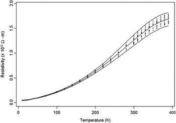
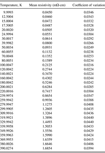
The electrical resistivity was measured on 6 of the 10 SRM artifacts using the AC transport option of the Quantum Design PPMS. A standard four-point probe technique was used. Figure 12 shows the resistivity data as a function of temperature; these data are also tabulated in Table IV.
SRM artifact resistivity as a function of temperature showing mean values and 95% confidence intervals.

Electrical resistivity data for SRM 3451.

Four-probe Hall measurements were conducted at 300 K on a representative artifact sliced (using a wire saw) into the dimensions 0.5 mm × 2.5 mm × 8 mm, using the PPMS infrastructure and a custom measurement sequence. The Hall resistance, RH, was measured as a function of multiple positive and negative magnetic fields (−2.5 T < B < 2.5 T) to mitigate voltage probe misalignment effects and thermal instabilities. RH values for matching ±B were averaged using multiple zero field measurements. Using the relation n = 1/[(RH/B)(et)],Reference Kittel19 where RH/B is the fitted slope for the collection of RH and B values, n the carrier concentration, e the charge per carrier, and t the sample thickness, the carrier concentration is calculated to be 1.4 × 1019 cm-3.
VI. CONCLUSIONS
In conclusion, we have certified a SRM for low-temperature Seebeck coefficient measurements. The availability of this SRM will improve and validate measurement accuracy, leading to a better understanding of the structure/property relationships and underlying physics of new and improved thermoelectric materials.
ACKNOWLEDGMENTS
The authors acknowledge the partial financial support from the former Materials Science and Engineering Laboratory (currently Material Measurement Laboratory) of NIST. The assistance of S. Claggett for sample preparation of the interface layers of one of the SRM artifacts is also acknowledged.