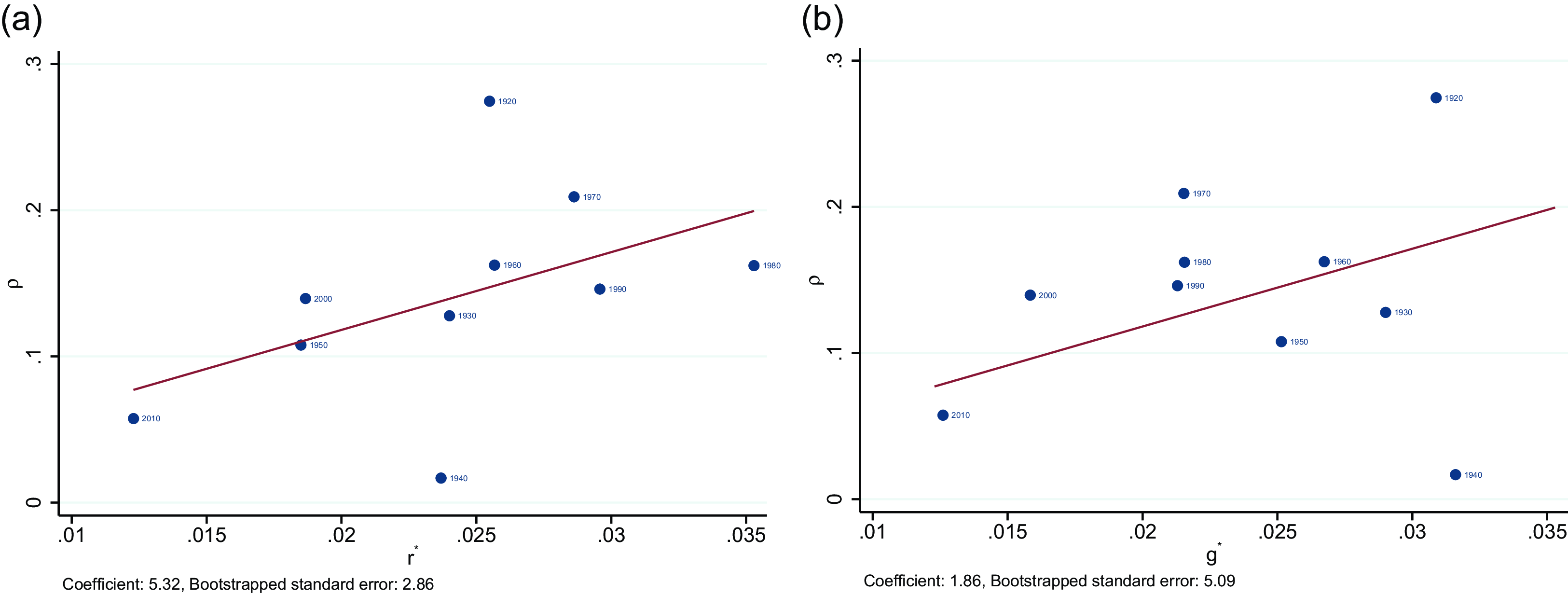
1. Introduction
Chronic or persistent budget deficits that produce mounting debt-GDP ratios pose grave concerns for most countries. In response to these concerns, governments usually take corrective actions for debt by increasing taxes and/or cutting spending. Such actions, characterized with a “fiscal reaction” function (Bohn, Reference Bohn1998) that relates the primary surplus to the debt, form the underlying framework for modern analysis of fiscal sustainability (see, e.g., Canzoneri et al. Reference Canzoneri, Cumby and Diba2001; Mendoza and Ostry, Reference Mendoza and Ostry2008; Collignon, Reference Collignon2012; Ghosh et al. Reference Ghosh, Kim, Mendoza, Ostry and Qureshi2013; Mauro et al. Reference Mauro, Romeu, Binder and Zaman2015; D’Erasmo et al. Reference D’Erasmo, Mendoza and Zhang2016). A simple expression of this function (from Bohn, Reference Bohn1998) is
 $s_t = \rho d_t + \mu _t$
, where
 $s_t$
is the primary surplus-GDP ratio at time
 $t$
,
 $d_t$
is the debt-GDP ratio at the beginning of time
 $t$
,
 $\rho$
is the fiscal reaction or feedback coefficient, and
 $\mu _t$
captures all other determinants of the primary surplus in time
 $t$
.Footnote
1
In this framework, the reaction coefficient
 $\rho$
, measuring the degree of the government’s willingness to respond to changes in debt, is a key parameter determining fiscal sustainability and hence its proper estimation is essential in making appropriate policy analyses or decisions.
The fiscal reaction function described above, though commonplace in fiscal sustainability studies, is predicated on an implicit assumption that the reaction coefficient is constant over time. This, however, may not necessarily be the case. In fact, the fiscal reaction function with a constant coefficient may not adequately describe the government’s fiscal behavior with respect to debt, and hence, it may be too limited to properly assess fiscal sustainability. To correct this problem, there is a growing body of empirical work on fiscal sustainability that allows for the time-varying nature of the fiscal reaction function. Collignon (Reference Collignon2012) uses recursive estimation of the fiscal reaction model and finds evidence for a structural break in the reaction coefficient for a number of European countries, largely dated around the signing of the Maastricht treaty. D’Erasmo et al. (Reference D’Erasmo, Mendoza and Zhang2016) also report evidence supporting a structural break in the U.S. coefficient around the time of the Great Recession. Burger and Marinkov (Reference Burger and Marinkov2012) and Aldama and Creel (Reference Aldama and Jérôme2017) estimate switching regression models to account for variation over time in the coefficient in the fiscal reaction function. Davig and Leeper (Reference Davig and Leeper2006), Davig and Leeper (Reference Davig and Leeper2011), and Bianchi and Ilut (Reference Bianchi and Ilut2017) study the interaction between monetary and fiscal policies, considering regime-switching processes in the fiscal rule with the tax rate. These results clearly attest to the importance of allowing for time variation in fiscal policy rules when analyzing fiscal sustainability. However, it is not easy to identify regime-switching processes in switching regressions and, more importantly, even where there is switching, the parameters governing the time series process remain constant, a possibly restrictive assumption.
In this paper, we present an altogether different approach to estimating the time-varying fiscal reaction function and, in so doing, we offer new insights into the study of fiscal sustainability. We model the time variation in the fiscal reaction coefficient as dependent on observable and unobservable factors, and demonstrate how the constant coefficient assumption can impact the determination of sustainable debt-GDP ratios. We postulate that the government’s fiscal response to changes in debt is likely to be influenced by persistent changes in economic conditions, as well as the political environment it is facing. In particular, we argue that a different economic environment calls for a different fiscal response to changes in debt. Mendoza and Ostry (Reference Mendoza and Ostry2008), in their cross-sectional study of model-based sustainability tests, suggest that changes in economic fundamentals (such as higher potential output growth rates) might lead to changes in the fiscal reaction coefficient. Mauro et al. (Reference Mauro, Romeu, Binder and Zaman2015) also find that variation in the fiscal reaction coefficient across countries is driven in part by unexpected changes in potential economic growth and sovereign borrowing costs. Garín et al. (Reference Garín, Lester, Sims and Wolff2019) discuss how a government’s budget decisions in the presence of low interest rates ought to depend on why exactly interest rates are low (a low potential growth rate has different implications than a greater desire on the part of the society to save). Furthermore, a number of studies have pointed to political determinants of surpluses or deficits (e.g., Alesina and Tabellini, Reference Alesina and Tabellini1990, Goff and Tollison, Reference Goff and Tollison2002), implying that a changing political environment might lead the government to alter its willingness to run surpluses in order to pay down debt.
Importantly, these considerations would suggest that the fiscal response to debt might be endogenously determined with a time-varying stochastic process. There are a few studies that allow the fiscal reaction coefficient to evolve endogenously. Chang and Kwak (Reference Chang and Kwak2017), in a related work, estimate endogenous regime-switching fiscal reaction functions with the tax rule using a time-varying VAR model where the fiscal parameters can endogenously switch across regimes based on latent factors, but their analysis is still based on a constant coefficient framework. Cimadomo et al. (Reference Cimadomo, Garnier and Schalck2007) use state space techniques to estimate time-varying fiscal reaction coefficients, but they impose a random walk on the reaction coefficient, not allowing for endogeneity.Footnote 2
To formalize the above arguments, we develop a generalized fiscal reaction function with a time-varying reaction coefficient that is allowed to vary with the interest rate and growth rate, as well as other, unobservable, factors. This enables us to analyze the dynamic behavior of government debt and deficits in a more comprehensive manner than in earlier studies. With this work, we make contributions to the study of fiscal sustainability on both theoretical and empirical grounds. On the theoretical side, with the generalized fiscal reaction function, we provide a full analysis of debt dynamics by deriving a stability condition that ensures a sustainable path of the debt-GDP ratio toward a long-run or steady state value. Then, we examine the effects of the interest rate and growth rate on the steady state debt-GDP ratio. The fiscal reaction function with a constant reaction coefficient implies that an increase in the economy’s growth rate lowers the steady state debt-GDP ratio, while an increase in the interest rate raises the steady state debt-GDP ratio. When the reaction coefficient evolves endogenously with growth rates or the interest rate, this may not hold. Further, we analyze the long-run relationship between the primary surplus or deficit and the debt-GDP ratio, which describes the fraction of GDP that the government needs to save in order to service debt in the steady state. An important finding is that when interest rates are low relative to growth rates, frequent or chronic budget deficits can be consistent with a sustainable debt.
In the empirical analysis, we present a state space model to estimate the generalized time-varying fiscal reaction function, treating the reaction coefficient as an unobservable stochastic process. The state space approach is also useful, given that we argue that the government’s corrective actions with respect to increasing debt is based on the natural rate of interest and the potential output growth rate, both of which are unobservable. We specify the real interest rate as the sum of the natural rate of interest and a transitory or cyclical component, and we assume that it is correlated with the potential output growth rate, as well as other determinants (such as consumers’ preferences) that may evolve as random walks. The cyclical component of the interest rate is specified as an autoregressive distributed lag process. Observed real GDP is defined as the sum of unobservable trend and transitory (or cyclical) components. The trend follows a random walk with drift, and we interpret this drift as the rate of potential output growth. The state space model is estimated using the Kalman filter via Bayesian techniques, allowing for stochastic volatility of shocks, with the use of prior information, since the model is fairly heavily parameterized and the sample period is somewhat short.
We fit the state space model to the data on U.S. debt-GDP ratios over 1916 to 2022. Although there is evidence that the government considered long-term projections of the interest rate and the growth rate (especially the interest rate) in its fiscal decisions, the response to debt was largely driven by unobservable non-economic factors and by large and persistent shocks. Our results reveal that the federal government was actually more aggressive about containing the debt-GDP ratio for much of the postwar 20th century than would be suggested by the seminal estimates of Bohn (Reference Bohn1998). Specifically, while Bohn (Reference Bohn1998) estimated a reaction coefficient equal to 0.054, we find that, from the mid-1950s to the start of the Great Recession, the reaction coefficient hovered between 0.10 and 0.25 in magnitude. This contrasts with relatively lax estimated responses to debt stockpiles since the year 2009. Because our model controls for cyclical deviations of output and temporary military build-ups associated with wars, this increasing laxness cannot be attributed solely to the output losses of the Great Recession, the expenditures associated with early 21st century military conflicts, or the economic volatility generated by the COVID-19 pandemic. At the end of our sample period in 2022, the reaction coefficient is estimated to be close to the lowest it has been since the years following the end of World War II. The result is a rising steady state debt-GDP ratio.
2. A theoretical framework
When conducting fiscal policy, the government faces an intertemporal budget constraint, which is expressed as
 \begin{equation} D_{t+1} = (1+r)(D_t+G_t-T_t) = (1+r)(D_t-S_t), \forall t \geq 0 \end{equation}
where
 $D_t$
is the stock of government debt outstanding at the beginning of period
 $t$
,
 $r$
is the rate of interest,
 $G_t$
is government spending net of interest during period
 $t$
,
 $T_t$
is government revenue during period
 $t$
, and
 $S_t \equiv T_t-G_t$
is the “primary” budget balance or surplus at time
 $t$
, which is the difference between the government’s tax revenue and spending, net of interest payments. For ease of exposition, we assume for now that the interest rate is constant or stationary with a constant mean, but this assumption will be relaxed in the empirical analysis. We consider all variables in real terms.
An economy where GDP is growing rapidly has relatively more resources at its disposal with which to pay the principal and interest on its debts, so a pertinent measure of the government’s debt burden is not the level of debt itself, but the debt as a proportion of GDP, i.e., the debt-GDP ratio. Assume that the economy, as measured by GDP (denoted by
 $Y$
), grows at a rate of
 $g$
every period so that
 $Y_{t+1}=(1+g)Y_t, \forall t \geq 0$
. Then divide both sides of (1) by GDP to express the government budget constraint in terms of the debt-GDP ratio:
 \begin{equation} d_{t+1} = (1+\delta )(d_t-s_t), \forall t \geq 0 , \end{equation}
with
 $\lim _{N \to \infty } d_{N+1} \geq 0$
, where
 $d_t \equiv \frac {D_t}{Y_t}$
is the debt-GDP ratio,
 $s_t \equiv \frac {S_t}{Y_t}$
is the surplus-GDP ratio, and
 $1+\delta \equiv \frac {(1+r)}{(1+g)}$
, which gives
 $\delta \approx r-g$
, the growth-adjusted interest rate.
Taxes and spending, and hence surpluses, are not exogenously given in the government budget constraint. Rather, they are the government’s choice or policy variables, determined by some political process. We assume that the government takes corrective actions in its budget by increasing taxes and/or cutting spending in response to a higher debt-GDP ratio. This idea is described by the fiscal reaction function in (3) below and is incorporated into the government budget constraint in (2) to evaluate fiscal sustainability.
In its simplest form, as stated in Section 1, the fiscal reaction function of Bohn (Reference Bohn1998) takes the form:
 \begin{equation} s_t = \rho d_t + \mu _t, \forall t \geq 0 , \end{equation}
where
 $\rho$
is the reaction coefficient, and
 $\mu _t$
captures all other determinants of the primary surplus in time
 $t$
. We assume that
 $\mu _t\lt 0$
, because the government’s budget is considered to be in deficit, i.e.,
 $s_t\lt 0$
, without taking corrective actions (
 $\rho =0$
).Footnote
3
With corrective actions, the deficit can be reduced, leading to lower debt. Specifically, a positive value of
 $\rho$
means that the government takes corrective measures in response to a higher debt-GDP ratio in order to ensure solvency. Further, a positive, but large, value of
 $\rho$
indicates that the government is aggressive about countering the increase in debt, while a lower value implies that the government is less concerned about the debt increase.
As we argued in Section 1, the reaction coefficient
 $\rho$
measuring the degree of fiscal responsiveness to changes in debt need not have a fixed value, but instead might vary over time, possibly with changes in the interest rate and output growth rate, i.e.
 $\rho = f(r,g)$
.Footnote
4
For a given debt level, rising interest rates lead to larger debt service payments and may likely force the government into further fiscal adjustment in the form of tax hikes or spending cuts, thus necessitating larger budget surpluses. On the other hand, a higher growth rate can increase a country’s fiscal capacity and allow the government to have smaller surpluses in order to maintain a given debt-GDP ratio.
We propose for now that the reaction coefficient
 $\rho$
takes the following form:
 \begin{equation} \rho = \alpha _0 + \alpha _1 r + \alpha _2 g , \end{equation}
where
 $\alpha _0, \alpha _1,$
and
 $\alpha _2$
are coefficients to be estimated.Footnote
5
The parameter
 $\alpha _0$
reflects the part of the government’s response to changes in debt that occurs independently of changes in the interest rate and the growth rate. We hypothesize for the moment that
 $\alpha _0\gt 0$
,
 $\alpha _1\gt 0$
, and
 $\alpha _2\lt 0$
. A positive value of
 $\alpha _1$
can help explain the Mendoza and Ostry (Reference Mendoza and Ostry2008) conjecture that, in countries with riskier financial and fiscal environments (such as developing countries), where interest rates may be higher, the fiscal reaction coefficient is also higher, requiring larger budget surpluses or smaller budget deficits in these countries relative to GDP. On the other hand, low interest rates imply that borrowing is relatively cheap, which may allow the government to increase spending, generating larger budget deficits or smaller budget surpluses in relation to GDP.Footnote
6
A negative value of
 $\alpha _2$
, however, implies that the higher economic growth often observed in developing countries can make their reaction coefficients smaller than those of industrialized countries, leading to smaller budget surpluses or larger budget deficits in relation to GDP.
Substituting (4) into (3), we obtain
 \begin{equation} s_t = \alpha _0 d_t + \alpha _1 (r \times d_t) + \alpha _2 (g \times d_t) + \mu _t , \forall t \geq 0 , \end{equation}
which can be rewritten as
 \begin{equation} s_t = \alpha _0 d_t + \mu _t^m , \forall t \geq 0, \end{equation}
where
 $\mu _t^m \equiv \alpha _1 (r \times d_t) + \alpha _2 (g \times d_t) + \mu _t , \forall t \geq 0$
. Clearly, the fiscal reaction function (3) estimated in Bohn (Reference Bohn1998), with a constant
 $\rho$
, is a special case of the generalized fiscal reaction function (5) with an endogenous
 $\rho$
, if we let
 $\alpha _0=\rho$
and
 $\alpha _1=\alpha _2=0$
. In this case, we have the fiscal reaction function (6) that is of the same form as (3). This implies that when the fiscal reaction coefficient is endogenously determined, estimation of (3) instead of (5) likely produces a biased estimate of the reaction coefficient. Notably, (5) allows us to examine the effect of the interest rate and growth rate on the primary surplus. That is, for a given debt level,
 $\frac {\partial s_t}{\partial r} = \alpha _1 d_t \gt 0$
and
 $\frac {\partial s_t}{\partial g} = \alpha _2 d_t \lt 0$
. This suggests that policymakers may alter their behavior in response to changes in the interest rate or growth rate, which can affect the budget surplus or deficit. For the duration of the discussion of our conceptual framework, we will assume that the reaction coefficient in (3) takes the form in (4).
To investigate the dynamic behavior of the debt-GDP ratio, substitute (3) into (2) to get
 \begin{equation} d_{t+1} = \kappa d_t + w_t , \forall t \geq 0, \end{equation}
or, equivalently
 \begin{equation} \Delta d_{t+1} \equiv d_{t+1}-d_t = -(1-\kappa )d_t + w_t , \forall t \geq 0, \end{equation}
where
 $\kappa \equiv (1+\delta )(1-\rho )$
and
 $w_t \equiv -(1+\delta ) \mu _t$
, with
 $\mu _t \lt 0$
. (7) is a first-order difference equation with a forcing variable
 $w_t$
, and the stability condition requires that
 $-1 \lt \kappa \lt 1$
. It is common to use an approximation for
 $\kappa$
, with
 $\delta \approx r-g$
(Bohn, Reference Bohn1998; Mendoza and Ostry, Reference Mendoza and Ostry2008; Collignon, Reference Collignon2012). Further, for small values of
 $\delta$
and
 $\rho$
,
 $\kappa \approx 1+\delta -\rho$
. The stability condition then requires that
 $r-g \lt \rho$
. In the interests of a more precise analysis, we instead use an exact expression for
 $\kappa$
with
 $1+\delta = \frac {(1+r)}{(1+g)}$
. Then, the stability condition takes the form
 $\frac {(r-g)}{(1+r)} \lt \rho$
. Since the stability condition ensures the sustainability of debt, we state the following:
Proposition 1.
Given that the government takes corrective actions for a rising debt, the viable condition for fiscal sustainability requires that
 $\frac {(r-g)}{(1+r)}\lt \rho$
. For
 $ r \lt g$
, this condition is satisfied for a positive value of
 $\rho$
. When the sustainability condition is satisfied, the debt-GDP ratio has a stable, convergent path toward a steady state (with a non-negative value), and the government’s debt or fiscal position is sustainable. If the fiscal position is not sustainable, the debt-GDP ratio is explosive or continues to grow with no bound.
To assess the government’s fiscal position, it is crucial to take into account its corrective actions for a rising debt. In Appendix A, we show that the failure to do so leads to an improper sustainability condition and hence misleading inference about fiscal sustainability. While the sustainability condition formalized above is also recognized in previous studies (see, e.g., Mendoza and Ostry, Reference Mendoza and Ostry2008, Collignon, Reference Collignon2012, or Ghosh et al. Reference Ghosh, Kim, Mendoza, Ostry and Qureshi2013), it is based on a constant reaction coefficient. In our model, the reaction coefficient is endogenously determined, allowing for a better understanding of the budgetary adjustment mechanism that underlies fiscal sustainability in response to changes in the interest rate or the output growth rate.
The stability condition ensures a convergent path of the debt-GDP ratio toward a long-run or steady state value. The steady state value can be obtained by setting
 $\Delta d_{t+1} = 0$
in (8) and solving for
 $d$
.Footnote
7
Assuming that the value of
 $w_t$
is constant at
 $w$
over time (implying a constant value of
 $\mu$
), the steady state value of the debt-GDP ratio is given by
 \begin{equation} \bar {d} = \frac {w}{1-\kappa } = \frac {-(1+r)\mu }{(1+g)-(1+r)(1-\rho )}\ . \end{equation}
For a stable solution, a positive steady state debt-GDP ratio requires that
 $\mu \lt 0$
.Footnote
8
With this steady state debt-GDP ratio, the solution to (7) is
 \begin{equation} d_t - \bar {d} = \kappa ^t(d_0-\bar {d}) , \forall t \geq 0\ . \end{equation}
This equation describes the trajectory of the debt-GDP ratio over time toward the steady state. Substituting the value of
 $d_t$
from (10) into (3), we also obtain the time path of the primary surplus over time. Equation (10) reveals the mean-reverting process of the debt-GDP ratio, with the mean being the steady state value,
 $\bar {d}$
. Note that
 $(d_t-\bar {d})$
is the deviation of the debt-GDP ratio from its steady state value at time
 $t$
. Equation (10) suggests that a fraction of this deviation tends to decay each period with the government’s corrective fiscal actions, absent any further shock, at a constant rate
 $1-\kappa$
. Whether an increase in the interest rate or growth rate increases or decreases the rate of convergence to the steady state depends on its effect on the steady state debt-GDP ratio.
It is commonly claimed that higher economic growth will reduce the steady state debt-GDP ratio (and lower economic growth will raise the steady state debt-GDP ratio); see, for example, Bohn (Reference Bohn1995) or Collignon (Reference Collignon2012). To assess the effect of changes in economic conditions on debt dynamics, we can evaluate the steady state debt-GDP ratio (9), assuming a fiscal reaction function with a constant value of
 $\rho$
. Taking derivatives of this expression with respect to the interest rate and the growth rate, we have
 \begin{equation} \frac {\partial \bar {d}}{\partial r} = \frac {-(1+g)\mu }{[(1+g)-(1+r)(1-\rho )]^2} \gt 0 \end{equation}
and
 \begin{equation} \frac {\partial \bar {d}}{\partial g} = \frac {(1+r)\mu }{[(1+g)-(1+r)(1-\rho )]^2} \lt 0 , \end{equation}
because
 $\mu \lt 0$
. Equation (11) shows that an increase in the interest rate raises the steady state debt-GDP ratio. Equation (12) clearly supports the claim that high economic growth lowers the debt-GDP ratio (Collignon, Reference Collignon2012).
Such a claim, however, is dependent on a constant reaction coefficient and fails to account for the possibility that the growth rate might affect the coefficient, as indicated in (4). A generalized fiscal reaction function with an endogenous reaction coefficient allows us to undertake a more comprehensive examination of this issue. With
 $\rho$
of the form in (4), the steady state debt-GDP ratio will depend on
 $r$
and
 $g$
not only in the direct fashion described by (11) and (12), but also indirectly through their effect on
 $\rho$
. All else constant, a higher reaction coefficient
 $\rho$
reduces the steady state debt-GDP ratio, because the government responds with larger primary surpluses, as opposed to borrowing, when debt rises. To examine the effect of the interest rate and growth rate on the steady state debt-GDP ratio, we assume a general form of the fiscal reaction coefficient, i.e.,
 $\rho = f(r,g)$
and, taking derivatives of
 $\bar {d}$
in (9) with respect to
 $r$
and
 $g$
,Footnote
9
we get
 \begin{equation} \frac {\partial {\bar {d}}}{\partial {r}} = \frac {[-(1+g)+(1+r)^2 f_r (r,g)]\mu }{\left[(1+g)-(1+r)(1-f(r,g))\right]^2} \end{equation}
and
 \begin{equation} \frac {\partial {\bar {d}}}{\partial {g}} = \frac {(1+r)[1+(1+r) f_g (r,g)]\mu }{\left[(1+g)-(1+r)(1-f(r,g))\right]^2}. \end{equation}
Note that (11) and (12) are special cases of (13) and (14) when
 $f_r (r,g) = f_g (r,g) = 0$
. Unlike in the case of (11) and (12), however, the signs of the derivatives in (13) and (14) are not known. Since
 $\mu \lt 0$
, evaluating these expressions requires knowing whether the terms in brackets in the numerators are positive or negative. For
 $r$
, then, we get the following condition:
 \begin{equation} \frac {\partial \bar {d}}{\partial r} \gtreqless 0\ \text{if}\ f_r (r,g) \lesseqgtr \frac {1+g}{\left(1+r\right)^2} \end{equation}
We obtain a similar condition for
 $g$
:
 \begin{equation} \frac {\partial \bar {d}}{\partial g} \gtreqless 0\ \text{if}\ f_g (r,g) \lesseqgtr \frac {-1}{1+r} \end{equation}
In order to further derive the implications of these conditions, we examine the generalized fiscal reaction function in (4). We are assuming presently that
 $f_r (r,g) = \alpha _1\gt 0$
, so this in effect measures the influence of the interest rate on the primary surplus for any given level of debt.Footnote
10
We also suppose that
 $f_g (r,g) = \alpha _2\lt 0$
, measuring the influence of the growth rate on the primary surplus for any given debt level. This discussion gives an indication of how the government’s adjustment of its primary surplus in response to a change in the interest rate or the growth rate determines the steady state debt-GDP ratio. This leads to an important finding of our analysis:
Proposition 2. An increase in the growth rate of output can either raise or lower the steady state debt-GDP ratio. This is in sharp contrast to the common view that an increase in the growth rate lowers the steady state debt-GDP ratio. Whether an increase in the growth rate raises or lowers the steady state debt-GDP ratio depends on the degree of responsiveness of the primary surplus for a given debt level with respect to an increase in the growth rate; a higher degree of fiscal responsiveness allows a country to have a lower debt-GDP ratio. Similarly, an increase in the interest rate can raise or lower the steady state debt-GDP ratio. Whether an increase in the interest rate raises or lowers the steady state debt-GDP ratio depends on the degree of responsiveness of the primary surplus for a given debt level with respect to an increase in the interest rate; a lower degree of fiscal responsiveness allows a country to have a higher debt-GDP ratio.
While an increasing debt-GDP ratio can be sustainable as long as the stability condition is satisfied, a constant or steady state debt-GDP ratio is always sustainable by definition, because it is stationary, meaning that the debt will never explode. Assuming that the debt-GDP ratio is at its steady state value, we can solve for the primary surplus that supports it by letting
 $d_{t+1}=d_{t}=\bar {d}, \forall t \geq 0$
, in (2). Solving for
 $s_t$
, we obtain the following result:
Proposition 3. Suppose that the debt-GDP ratio reaches the steady state value. Then, the following equation describes the long-run relationship between the primary surplus or deficit and government debt:
 \begin{equation} \bar {s} = \frac {(r-g)}{(1+r)} \bar {d} , \end{equation}
which is the fraction of GDP that the government needs to save, i.e., the primary budget surplus, in order to service debt in the steady state. It is equal to the discounted growth-adjusted interest payments on a sustainable stock of debt.
Equation (17) shows that the spread between
 $r$
and
 $g$
, combined with the debt-GDP ratio, helps to determine the steady state budget deficit or surplus. If
 $r\gt g$
, the government must maintain a primary surplus in order to keep a constant debt-GDP ratio. If, however,
 $r\lt g$
, the government may run a primary deficit in every period while keeping the debt-output ratio constant. If
 $g=0$
, (17) describes a fraction of GDP for interest payments that the government is required to pay in order to service a given debt-GDP ratio. Figure 1 illustrates the relationship between the primary surplus-GDP ratio and the debt-GDP ratio in the steady state. It shows that to keep the debt-GDP ratio constant at the steady state value,
 $r\gt g$
requires a primary surplus, whereas
 $r\lt g$
implies a primary deficit. An implication of this result is that frequent or chronic budget deficits are consistent with a sustainable debt if
 $r\lt g$
.
Long-run relationship between the primary surplus/Deficit and debt.
Notes: The figure plots the relationship between the steady state debt-GDP ratio and the steady state surplus-GDP ratio, depending on whether the natural rate of interest is greater than or less than the potential output growth rate.

In (17), the steady state debt-GDP ratio
 $\bar {d}$
is not exogenously determined. To assess the effect of a change in the interest rate or the growth rate on the steady state primary surplus-GDP ratio, we need to allow for the effect of either variable on the steady state debt-GDP ratio. To do so, substitute (9) into (17) to get
 \begin{equation} \bar {s} = \frac {-(r-g)\mu }{(1+g)-(1+r)(1-f(r,g))}\ . \end{equation}
Figure 2 demonstrates how an increase in the growth rate can affect the steady state primary surplus-GDP ratio in the case that the growth rate is already greater than the interest rate. Higher growth causes the debt-GDP ratio to rise from
 $\bar {d}_1$
to
 $\bar {d}_2$
, and it also leads to a shift in
 $\bar {s}$
from
 $\bar {s}_1$
to
 $\bar {s}_2$
. We have focused on the effects of changes in the growth rate, but Figure 2 can also aid in understanding the effect of changes in the interest rate on the primary surplus-GDP ratio and the debt-GDP ratio in steady state. In this case, the effects are opposite of those of a change in the growth rate. These results are worth summarizing as follows:
Proposition 4.
A country may be able to sustain a large budget deficit in the steady state if its growth rate is high relative to its interest rate. For a sufficiently large derivative of
 $f(r,g)$
with respect to
 $r$
and for a sufficiently small derivative of
 $f(r, g)$
with respect to
 $g$
, an increase in the growth rate or a decline in the interest rate may allow a nation to have a yet higher sustainable debt-GDP ratio and higher steady state budget deficit.
Effects of an increase in the growth rate.
Notes: The figure plots how the steady state debt-GDP ratio and the steady state surplus-GDP ratio would respond to a permanent increase in the output growth rate.

The interest rate on government debt has been historically low relative to the growth rate of the economy, i.e.,
 $r\lt g$
, in most advanced economies (Mehrotra and Sergeyev, Reference Mehrotra and Sergeyev2021). This is expected to remain for a foreseeable future, especially for the United States. This unusual situation has prompted a reassessment of the government’s debt sustainability, with the possibility that the government may be able to engage in a Ponzi scheme for its debt (Ball et al. Reference Ball, Elmendorf and Mankiw1998; Blanchard, Reference Blanchard2019; Mehrotra and Sergeyev, Reference Mehrotra and Sergeyev2021). Our analysis offers a new perspective on this reassessment. Suppose that the government balances its primary budget every period and continues borrowing to pay for its interest payments on existing debt by rolling over its debt. Then, the debt-GDP ratio grows by
 $1+\delta = \frac {1+r}{1+g}$
(see (2)). If
 $r\lt g$
, the economy’s growth will dominate the rise in government debt due to rolling up interest, so while the debt-GDP ratio may increase for some time due to adverse shocks to growth or positive shocks to the interest rate, it will eventually decrease over time. Then, the debt could continue forever without an increase in the debt-GDP ratio, and the government with a large debt can most likely grow itself out of its problem, creating the possibility of a Ponzi scheme. In our analysis, we allow for the government’s corrective actions but do not require the government’s primary budget to be balanced. This entails
 $r\lt g$
with the debt-GDP ratio rising over time, reaching a non-negative steady state. Thus, continuous borrowing with budget deficits and persistent debt do not pose a problem for the government (see Section 2 for further discussion). Accordingly, with the government’s corrective actions, the possibility of a Ponzi scheme does not arise.
3. A state space model
The fiscal reaction function in (3) plays a central role in the analysis of fiscal sustainability. As discussed in Section 1, many existing studies estimate the fiscal reaction function by treating the reaction coefficient as a constant value, though some allow it to evolve over time. In Section 2, we argued that this reaction coefficient may, in fact, not be constant but rather endogenously determined or otherwise time-varying. In this section, we present a cogent empirical framework for implementing the generalized reaction function that is composed of (3) and (4). In Section 2, the theoretical model is formulated, for convenience, with constant interest rates and growth rates, as well as with constant values of the unmodeled determinants of the surplus-GDP ratio. In the empirical analysis, these variables are taken to vary over time, rendering crucial the time-varying nature of
 $\rho$
in our assessment of fiscal sustainability. In order to capture possibly time-varying behavior of fiscal policy, we propose modeling the evolution of the fiscal reaction coefficient in a state space framework, which also allows us to incorporate other important unobserved variables in the analysis. These may include changes in consumers’ preferences and political tastes, which can influence the reaction to debt stockpiles.
Equation (3) measures the responsiveness of the government’s fiscal policy to an increasing debt-GDP ratio, and this responsiveness is hypothesized to depend on the interest rate and the growth rate, and, we argue, particularly on long-term changes in the interest rate and growth rate. That is to say, a change in the potential output growth rate or the natural rate of interest is more likely to affect how fiscal policy responds to current debt ratios than would year-to-year realizations of observed GDP growth or interest rates. It is also likely that changes in the fiscal reaction coefficient will be persistent. Thus, we specify the fiscal reaction coefficient as a time-varying function of the following form:
 \begin{equation} \rho _t = \rho _{t-1} + \alpha _1 r_{t-1}^{*} + \alpha _2 g_{t-1}^{*} + e_t, \forall t \geq 0 \end{equation}
where
 $r_{t-1}^{*}$
is the natural rate of interest at period
 $t-1$
,
 $g_{t-1}^{*}$
is the potential output growth rate at period
 $t-1$
, and
 $e_t$
is an error term capturing unobservable shocks.Footnote
11
It is easy to imagine that other factors, such as political and social dynamics that are difficult to measure, can also affect how fiscal policy is set relative to a nation’s debt. Thus, we may desire that the fiscal reaction coefficient is itself subject to shocks, necessitating the inclusion of
 $e_t$
. The natural rate of interest and the potential output growth rate are unobservable.
The actual real interest rate is specified as the sum of the natural rate of interest and a transitory or cyclical component:
 \begin{equation} r_t = r_t^{*} + r_t^c, \forall t \geq 0\ \!. \end{equation}
For the natural rate of interest, we follow the work of Laubach and Williams (Reference Laubach and Williams2003) and specify it as
 \begin{equation} r_t^{*} = \gamma _1 g_{t}^{*} + \phi _{t}, \forall t \geq 0, \end{equation}
where
 $\phi _t$
captures unobservable determinants of
 $r_{t}^{*}$
, such as households’ rate of time preference (see also Lucas, Jr., Reference Lucas2003). Keeping in mind the critique of Garín et al. (Reference Garín, Lester, Sims and Wolff2019), we might interpret the
 $\gamma _1 g_t^{*}$
component of the real interest rate as capturing the endogenous effect of growth rates on interest rates, where a decline in this term implies that more borrowing is not in fact more affordable. The
 $\phi _t$
term captures a greater desire of agents to save, and interest rate reductions owing to a reduction in
 $\phi _t$
imply that borrowing is more affordable. It is implicitly a decline in
 $\phi _t$
that we analyzed in our theoretical sketch. We assume that this term follows a random walk:
 \begin{equation} \phi _t = \phi _{t-1}+\nu _t^{\phi }, \forall t \geq 0, \end{equation}
and
 $\nu _t^{\phi }$
is a white noise innovation term.Footnote
12
There is also a transitory or cyclical component of the real interest rate, which we specify as
 \begin{equation} r_t^c = \gamma _2 r_{t-1}^c + \gamma _3 y_{t-1}^c + \nu _t^c, \forall t \geq 0, \end{equation}
with
 $y_{t-1}^c$
the lagged cyclical component of real GDP and
 $\nu _t^c$
being a white noise innovation in the process.
The nominal interest rate (
 $i_t$
) is what we actually observe, and we set it equal to the sum of the real interest rate (
 $r_t$
), expected inflation (
 $\pi _t^e$
), and a forecast error, as follows:
 \begin{equation} i_t = r_t+\pi _t^e+\nu _{t}^{i}, \forall t \geq 0\ \!. \end{equation}
In order to infer inflation expectations in (24), we start with a typical Phillips Curve specification (Romer, Reference Romer2006, p. 257):
 \begin{equation} \pi _t = \pi _{t-1}^e + \gamma _4 y_t^c + u_{1,t}, \forall t \geq 0 , \end{equation}
where
 $\pi _t$
is the rate of inflation and
 $u_{1,t}$
captures supply-side shocks to inflation. The (unobserved) expected rate of inflation evolves in the following fashion:
 \begin{equation} \pi _t^e = \bar {\pi }+\gamma _5 \pi _{t-1}^e + u_{2,t}, \forall t \geq 0, \end{equation}
and
 $\bar {\pi }$
is the mean around which the stationary process for expected inflation fluctuates, while
 $u_{2,t}$
captures other unobservable factors.Footnote
13
In order to estimate the potential output growth rate (
 $g_t^{*}$
), we adopt the widely-used trend-cycle decomposition approach (see Clark, Reference Clark1987; Morley et al. Reference Morley, Nelson and Zivot2003; Kim and Murray, Reference Kim and Murray2002; Laubach and Williams, Reference Laubach and Williams2003) that expresses the logarithm of GDP (
 $y_t$
) as the sum of an unobservable trend component (
 $y_t^{\tau }$
) and a cyclical component (
 $y_t^c$
). The trend component is a random walk with drift, and we interpret the drift as the potential output growth rate. The cyclical component of output is a stationary process that has AR(1) dynamics and is also correlated with the lagged cyclical component of the real interest rate. Formally, we express the decomposition as
 \begin{align} y_t &= y_t^{\tau }+y_t^c, \forall t \geq 0\\[-10pt]\nonumber \end{align}
 \begin{align} y_t^{\tau } &= y_{t-1}^{\tau }+g_{t-1}^{*}+\eta _t^{\tau }, \forall t \geq 0\\[-10pt]\nonumber \end{align}
 \begin{align} g_t^{*} &= g_{t-1}^{*}+\eta _t^g, \forall t \geq 0\\[-10pt]\nonumber \end{align}
 \begin{align} y_t^c &= \gamma _6 y_{t-1}^c+\gamma _7 r_{t-1}^c+\eta _t^c, \forall t \geq 0 , \end{align}
and
 $\eta _t^{\tau }$
,
 $\eta _t^g$
, and
 $\eta _t^c$
are independent white noise processes.
Turning to the fiscal reaction function itself in (3), we postulate that the surplus-GDP ratio may deviate temporarily from the fiscal reaction rule because of the influence of other determinants, which may be unobservable. Following Bohn (Reference Bohn1998), we consider transitory fluctuations in output and in military spending, specifying the fiscal reaction function as
 \begin{equation} s_t = \delta _0 + \rho _t d_t + \delta _1 y_t^c + \delta _2 m_t^c + \delta _3 s_{t-1} + \theta _t, \forall t \geq 0, \end{equation}
where
 $\theta _t$
is an error term. The lagged surplus-GDP ratio is included to allow for possible serial correlation in the series. This is especially important, given the analysis in Leeper and Li (Reference Leeper and Li2017), who note that serial correlation in shocks to the surplus-GDP ratio would be a sufficient condition for regressions of the type estimated in Bohn (Reference Bohn1998) to be misleading. In order to estimate temporary deviations in real military spending (
 $m_t^c$
), we again apply a similar trend-cycle decomposition as for output. The log of real military spending,
 $m_t$
, can be expressed as
 \begin{align} m_t &= m_t^{\tau }+m_t^c, \forall t \geq 0\\[-10pt]\nonumber \end{align}
 \begin{align} m_t^{\tau } &= m_{t-1}^{\tau }+g_{t-1}^m + \omega _{t}^{\tau }, \forall t \geq 0\\[-10pt]\nonumber \end{align}
 \begin{align} g_t^m &= g_{t-1}^m + \omega _t^g, \forall t \geq 0\\[-10pt]\nonumber \end{align}
 \begin{align} m_t^c &= \gamma _8 m_{t-1}^c + \omega _t^c, \forall t \geq 0, \end{align}
where
 $\omega _t^{\tau }$
,
 $\omega _t^g$
, and
 $\omega _t^c$
are independent white noise processes. We include the transitory component of military spending to capture build-ups surrounding external conflicts like World War II and the wars in Korea and Vietnam.
For estimation, we cast the above set of equations as a state space framework. The state space model consists of the transition and measurement equations (see Kim and Nelson, Reference Kim and Nelson1999). For our empirical model, the transition equation describing the evolution of unobservable state variables is written as
 \begin{equation} \boldsymbol{\beta }_t = {\boldsymbol{C}}+{\boldsymbol{F}} \boldsymbol{\beta }_{t-1} +{\boldsymbol{E}}_t, \forall t \geq 0, \end{equation}
where
 \begin{equation*} \boldsymbol{\beta }_t \equiv \begin{bmatrix} \rho _t \\ \phi _t \\ r_t^c \\ \pi _t^e \\ y_t^{\tau } \\ g_t^{*} \\ y_t^c \\ m_t^{\tau } \\ g_t^m \\ m_t^c \\ \pi _{t-1}^e \\ \end{bmatrix}, {\boldsymbol{C}} \equiv \begin{bmatrix} 0 \\ 0 \\ 0 \\ \bar {\pi } \\ 0 \\ 0 \\ 0 \\ 0 \\ 0 \\ 0 \\ 0 \\ \end{bmatrix}, {\boldsymbol{F}} \equiv \left [\displaystyle \begin{array}{l@{\quad}c@{\quad}c@{\quad}c@{\quad}c@{\quad}c@{\quad}c@{\quad}c@{\quad}c@{\quad}c@{\quad}c} \displaystyle 1 & \alpha _1 & 0 & 0 & 0& \hat {\alpha _2} &0 & 0 & 0 & 0 & 0 \\ \displaystyle 0 & 1 & 0 & 0 & 0 & 0 & 0 & 0 & 0 & 0 & 0\\ \displaystyle 0 & 0 & \gamma _2 & 0 & 0 & 0 & \gamma _3 & 0 & 0 & 0 & 0 \\ \displaystyle 0 & 0 & 0 & 0 & 0 & 0 & 0 & 0 & 0 & 0& \gamma _5 \\ \displaystyle 0 & 0 & 0 & 0 & 1 & 1 & 0 & 0 & 0 & 0 & 0 \\ \displaystyle 0 & 0 & 0 & 0 & 0 & 1 & 0 & 0 & 0 & 0 & 0 \\ \displaystyle 0 & 0 & \gamma _7 & 0 & 0 & 0 & \gamma _6 & 0 & 0 & 0 & 0 \\ \displaystyle 0 & 0 & 0 & 0 & 0 & 0 & 0 & 1 & 1 & 0 & 0 \\ \displaystyle 0 & 0 & 0 & 0 & 0 & 0 & 0 & 0 & 1 & 0 & 0 \\ \displaystyle 0 & 0 & 0 & 0 & 0 & 0 & 0 & 0 & 0 & \gamma _8& 0 \\ \displaystyle 0 & 0 & 0 & 1 & 0 & 0 & 0 & 0 & 0 & 0 & 0 \\ \end{array}\right ], {\boldsymbol{E}}_t \equiv \begin{bmatrix} e_t \\ \nu _t^{\phi } \\ \nu _t^c \\ u_{2,t} \\ \eta _t^{\tau } \\ \eta _t^g \\ \eta _t^c \\ \omega _t^{\tau } \\ \omega _t^g \\ \omega _t^c \\ 0 \\ \end{bmatrix}, \end{equation*}
and
 $\hat {\alpha _2} = \alpha _1 \gamma _1 + \alpha _2$
. The measurement equation relates the observed data to the unobservable state variables:
 \begin{equation} {\boldsymbol{X}}_t = {\boldsymbol{H}}_t \boldsymbol{\beta }_t + {\boldsymbol{J}} {\boldsymbol{Z}}_t + \boldsymbol{\Xi }_t, \forall t \geq 0 , \end{equation}
where
 \begin{equation*} {{\boldsymbol{X}}}_t \equiv \begin{bmatrix} i_t \\ \pi _t \\ y_t \\ s_t \\ m_t \\ \end{bmatrix}, {\boldsymbol{H}}_t \equiv \left [\begin{array}{l@{\quad}c@{\quad}c@{\quad}c@{\quad}c@{\quad}c@{\quad}c@{\quad}c@{\quad}c@{\quad}c@{\quad}c} \displaystyle 0 & 1 & 1 & 1 & 0 & \gamma _1 & 0 & 0 & 0 & 0 & 0 \\ \displaystyle 0 & 0 & 0 & 0 & 0 & 0 & \gamma _4 & 0 & 0 & 0 & 1 \\ \displaystyle 0 & 0 & 0 & 0 & 1 & 0 & 1 & 0 & 0 & 0 & 0 \\ \displaystyle d_{t} & 0 & 0 & 0 & 0 & 0 & \delta _1 & 0 & 0 & \delta _2 & 0 \\ \displaystyle 0 & 0 & 0 & 0 & 0 & 0 & 0 & 1 & 0 & 1 & 0 \\ \end{array}\right ], {\boldsymbol{J}} \equiv \begin{bmatrix} 0 & 0 \\ 0 & 0 \\ 0 & 0 \\ \delta _0 & \delta _3 \\ 0 & 0 \\ \end{bmatrix}, \end{equation*}
 \begin{equation*} {\boldsymbol{Z}}_t \equiv \begin{bmatrix} 1 \\ s_{t-1} \\ \end{bmatrix}, \boldsymbol{\Xi }_t \equiv \begin{bmatrix} \nu _t^{i} \\ u_{1,t} \\ 0 \\ \theta _t \\ 0 \\ \end{bmatrix} . \end{equation*}
We assume that
 ${\boldsymbol{E}}_t \sim {\mathcal{N}} (0,\boldsymbol{Q})$
and
 $\boldsymbol{\Xi }_t \sim {\mathcal{N}} (0,\boldsymbol{R}_t)$
. In order to maintain the parsimony of the model, we assume that
 $\boldsymbol{Q}$
is a diagonal matrix and that the shocks to all of the various state variables are independent of each other at all leads and lags.Footnote
14
Since there is no error term associated with the lagged value of expected inflation, its variance is zero, meaning that
 $\boldsymbol{Q}$
is a collection of ten variance terms: [
 $\sigma ^2 (\rho _t)$
,
 $\sigma ^2 (\phi _t)$
,
 $\sigma ^2 (r_t^c)$
,
 $\sigma ^2 (\pi _t^e)$
,
 $\sigma ^2 (y_t^{\tau })$
,
 $\sigma ^2 (g_t^y)$
,
 $\sigma ^2 (y_t^c)$
,
 $\sigma ^2 (m_t^{\tau })$
,
 $\sigma ^2 (g_t^m)$
,
 $\sigma ^2 (m_t^c)$
]. There are three variance terms in the matrix
 $\boldsymbol{R}_t$
: [
 $\sigma _t^2 (i_t)$
,
 $\sigma _t^2 (\pi _t)$
,
 $\sigma _t^2 (s_t)$
], and while we assume that
 $\boldsymbol{R_t}$
is also diagonal, we allow for stochastic volatility so that the non-zero terms in
 $\boldsymbol{R_t}$
evolve over time. The reason for this is that, in models with time-varying parameters where stochastic volatility is not allowed for, it is possible to spuriously estimate variation in parameters over time when it is actually the volatility of shocks changing over time (see Fernández-Villaverde et al. Reference Fernández-Villaverde, Guerrón-Quintana, Kuester and Rubio-Ramírez2015; Chang and Kwak, Reference Chang and Kwak2017).
4. Estimation and results
4.1. Data
We estimate the state space model in order to assess the sustainability of U.S. federal government debt over the years from 1916 to 2022.Footnote 15 Most of our data comes from standard sources (i.e., information on real GDP and real military spending is obtained from the Bureau of Economic Analysis, while the debt-GDP and surplus-GDP ratios are taken from the U.S. Office of Management and Budget). For the interest rate, we use the yield on the 10-year Treasury note. To extend the data set to 1916 (the first year analyzed in Bohn (Reference Bohn1998)), we obtain information on most of the key variables for our model from the online database associated with Bohn (Reference Bohn and Bohn2008). The one exception to that rule is that, to extend the data set for the yield on the 10-year Treasury note, we use the database published alongside Shiller (Reference Shiller1989) and Shiller (Reference Shiller2015).
Figure 3a reports the time series of the debt-GDP ratio over the course of our sample period. The debt-GDP ratio is generally rising between 1916 and the end of World War II, peaking above 100 percent of GDP before falling dramatically over a span of decades. It begins to rise in the 1980s, falls in the late 1990s, and has generally been increasing since the turn of the new millennium, with a sharp turn upwards as the pandemic struck. Figure 3b offers an analogous depiction of the primary budget surplus as a share of GDP. The time series is characterized by large negative values, i.e., primary budget deficits, that occurred during World War I, World War II, the Great Recession of 2007 to 2009, and in 2020. Outside of these episodes, the surplus-GDP ratio tends to hover around zero, although there is a very subtle negative trend in the series since the start of the 1950s. A negative trend in the surplus combined with rising debt would seem to support the idea that the relationship between the two series has been changing over time.
Debt- and surplus-GDP ratios.
Notes: The left figure plots the time series of U.S. government debt held by the public as a share of Gross Domestic Product. The right figure plots the time series of U.S. government primary surplus as a share of Gross Domestic Product.

4.2. Model parameter estimates
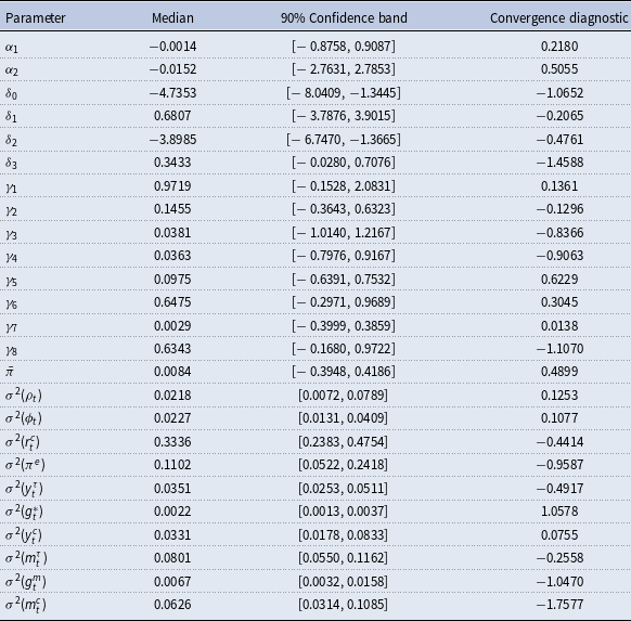
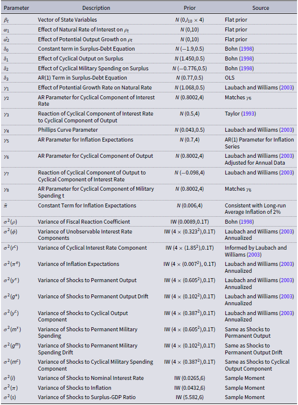
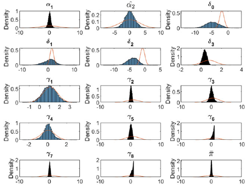
We use the Kalman filter and Bayesian statistical methods to estimate the model presented in Section 3. Appendix B reports our estimation algorithm, allowing for stochastic volatility of shocks. Bayesian methods incorporate prior knowledge on the behavior of some of the dynamic relationships that may help to produce more efficient estimates. Appendix Table D1 contains the prior distributions for each of the parameters in the state space model, and Appendix Figure E1. depicts the posterior distributions of these model coefficients with histograms. For comparison, the figures offer the kernel densities of the prior distributions of each parameter as well. Table 1 contains the same results in tabular form, reporting the median, as well as the
 $5^{th}$
and
 $95^{th}$
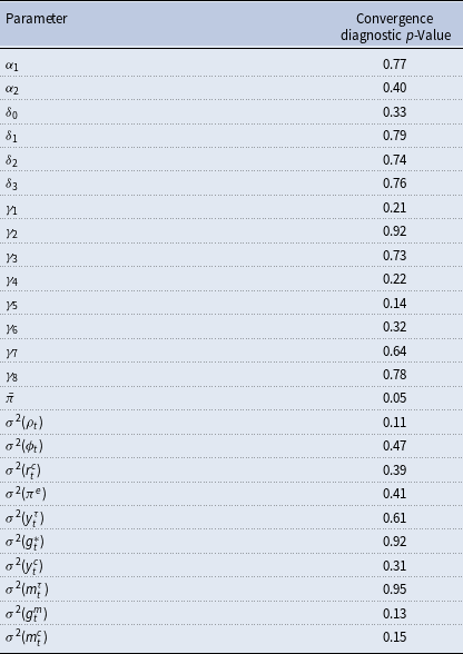
percentiles, of the posterior distribution, alongside a convergence diagnostic statistic which tests for the equality of means of the parameter in the first 10 percent of retained draws and the last 40 percent of retained draws (that is, after the burn-in period). This statistic assesses the extent to which the influence of the initial parameter guess has been purged. Table 1 shows that we cannot reject the null of no difference in means in the two different parts of the distribution for all but one of the parameters at the 5 percent significance level after the burn-in period, which implies that the estimation has generally converged. As a robustness check, we also considered two other convergence diagnostics discussed in Appendix C, which show convergence.
Parameter posterior distributions

Notes: The table reports the main statistics associated with the simulated posterior distribution for each parameter in the model. The convergence diagnostic is defined as
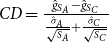 $CD = \frac {\hat {g}_{S_A} - \hat {g}_{S_C}}{\frac {\hat {\sigma }_{A}}{\sqrt {S_A}}+\frac {\hat {\sigma }_C}{\sqrt {S_C}}}$
; see Koop (Reference Koop2003). The convergence diagnostic statistics are compared with standard normal critical values.
 $\hat {g}$
is the average value of each parameter over the first 10% of draws after the burn-in period (
 $S_A$
) or the last 40% of draws after the burn-in period (
 $S_C$
). Failure to reject the null implies convergence of the draws to the posterior distribution.
Inference on latent variables.
Notes: The top left figure reports the estimated time series of the natural rate of interest (
 $r^{*}$
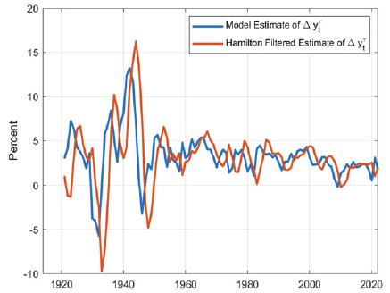
) from the state space model discussed in Section 3. For comparison, we also include the natural rate of interest implied by applying the filter introduced in Hamilton (Reference Hamilton2018). For the Hamilton filter, we use the modified specification of Quast and Wolters (Reference Quast and Wolters2022), in which the projection horizon is varied from 1 to 3 years, with one lag in all regressions. The values we use are the average of the Hamilton cyclical component derived from the 1-year-ahead, 2-year-ahead, and 3-year-ahead projection horizons. The top right figure reports the estimated time series of the potential output growth rate (
 $g^{*}_t$
) from the state space model discussed in Section 3, alongside the growth rate of measured output (
 $g_t$
). The bottom figure depicts the time series of
 $\sigma _t^2 (s_t)$
, the variance of the error term in the surplus-GDP ratio equation.

The state space model provides estimates of the natural rate of interest and the potential output growth rate, which we use to estimate the fiscal reaction coefficient
 $\rho _t$
, as well as the steady state debt-GDP ratio and surplus-GDP ratio. Figure 4a presents the actual and natural rates of interest,Footnote
16
and Figure 4b depicts the actual output growth rate and the potential output growth rate.Footnote
17
Although there is considerable variability over time in the actual real interest rate and real output growth rate, the estimated latent long-run values are comparatively stable over time and are comparable to the estimates of Laubach and Williams (Reference Laubach and Williams2003), despite the context being different.
Turning to the parameter estimates themselves, we first note that neither
 $\alpha _1$
nor
 $\alpha _2$
is statistically significant and both are very close to zero, indicating that changes in the natural rate of interest or the potential output growth rate do not have a strong influence on the way fiscal policymakers react to debt ratios at this frequency.Footnote
18
Importantly, however, the variance of innovations to the fiscal reaction coefficient (
 $\sigma _{\rho }^2$
) is 0.0221. This is approximately 40.9 percent of the estimated
 $\rho$
coefficient (0.054) in Bohn (Reference Bohn1998). This is an indication that large and persistent exogenous shocks to the fiscal reaction coefficient are an important driver of its fluctuations, a subject we turn to in the next subsection.
Looking at the other parameters of the fiscal reaction function, as expected, the surplus is serially correlated, with an AR(1) parameter (
 $\delta _3$
) of 0.3597, and it is positively associated with the cyclical component of GDP (with
 $\delta _1=0.7511$
) and negatively associated with the transitory component of military spending (
 $\delta _2=-3.9856$
), significant at the ten percent significance level and implying that the government is willing to run large deficits in wartime. These results accord well with our intuition.
In Figure 4c, we report the time series of
 $\sigma _t^2 (s_t)$
, or the estimated conditional variance of innovations in the surplus-GDP ratio. It is evident that the long-run trend in variability of the surplus-GDP ratio is downward, compared with the years around World War I and World War II. That said, it is also clear that the variance of the surplus-GDP ratio has risen recently, with a slow increase since the 1980s. Fernández-Villaverde et al. (Reference Fernández-Villaverde, Guerrón-Quintana, Kuester and Rubio-Ramírez2015) estimate tax and spending processes for the United States with time-varying volatility, and they find that unexpected changes in fiscal volatility can affect economic activity. As of the end of our sample,
 $\sigma _t^2 (s_t)$
was still higher than it had been for most of the postwar period. This suggests that time-varying volatility in shocks to the surplus-GDP ratio, while possibly very important in earlier periods, has played less of a role in recent decades, at least before the Great Recession.Footnote
19
4.3. Main results
In this section, we report the results for fiscal sustainability implied by estimation of the state space model.
Evolution of fiscal reaction coefficient.
Notes: The figure reports the estimated time series of the coefficient on the debt-GDP ratio (
 $\rho$
in the model discussed in Section 3) from the state space model for the full sample and the post-WWII period. 90 percent confidence band is denoted by the dashed line. Light blue shading indicates periods when the debt-GDP ratio is not sustainable.

4.3.1. Evolution of the fiscal reaction coefficient
Figure 5 illustrates the evolution over time of the fiscal reaction coefficient, which relates the surplus-GDP ratio to the debt-GDP ratio and is a key element in fiscal sustainability analysis, along with 90 percent confidence bands. The figure also, for comparison, shows the estimated value of
 $\rho =0.054$
in Bohn (Reference Bohn1998), as well as an updated coefficient of 0.002.Footnote
20
Our results indicate that, in many periods in the last 100 years, the government was actually more proactive about constraining increases in the debt-GDP ratio than even the rather robust results of Bohn (Reference Bohn1998) might have implied. In the years before the onset of the Great Depression,
 $\rho$
generally stayed well above 0.1, reaching as high as about 0.32 in 1929. During the Depression years and into World War II, however,
 $\rho$
collapsed, hitting a trough of around
 $-0.20$
in 1943. The implication is that the large deficits run by the federal government during this period were not solely a result of deviations of output or military spending from their respective trends, but also reflected a reduction in aggressiveness in working to counteract debt build-ups. In other words, big increases in demand for military spending during the war led to higher deficits for any given debt level, but even without the war spending, the government would not have tried to run a higher surplus in response to higher debt.
Following the war,
 $\rho$
rises steadily, hitting a local peak around 0.26 (about two tenths higher than the average estimate of Bohn, Reference Bohn1998) in 1974, and then begins to trend downward. The decline is particularly steep after the turn of the millenium, suggesting that, over the last two decades, policymakers have become less concerned about debt as a motivating factor to rein in deficits. Notably, since the end of the Great Recession, the reaction coefficient has hovered around the value of 0.05. In 2022, the last year of our sample,
 $\rho = 0.0498$
, close to the lowest value since World War II, with the exception of the Great Recession years and the 2020 pandemic year. Our model thus implies that the agressiveness with which policymakers react to debt is currently near the lowest in the modern era.
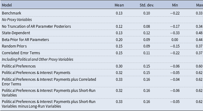
It is worth noting that, in our baseline estimation, the average value of
 $\rho$
is 0.13, and this average coefficient value is robust to a number of different specifications that we consider, as discussed in Appendix C.Footnote
21
However, this value is larger than that of Bohn (Reference Bohn1998) and other previous studies for much of the sample. This may reflect differences in methodology used to estimate the fiscal reaction function. Previous studies, by and large, estimate this function with a constant coefficient. Our analysis, in contrast, has demonstrated the importance of the time-varying, endogenous nature of the reaction coefficient, along with the stochastic volatility of shocks to the surplus-GDP ratio.Footnote
22
It is also important at this point that we address the critique of Leeper and Li (Reference Leeper and Li2017), who argue that single-equation surplus-debt regressions may provide misleading inference on the fiscal reaction coefficient when monetary policy is passive and fiscal policy is active, which is likely to cover much of our sample period.Footnote 23 In the terminology of Leeper and Li (Reference Leeper and Li2017), monetary policy is said to be passive when the policy interest rate reacts only weakly to inflation, or the coefficient on inflation in a Taylor (Reference Taylor1993)-type rule is less than one in absolute value. Fiscal policy is said to be active when the absolute value of the fiscal reaction coefficient is less than one. Leeper and Li (Reference Leeper and Li2017) argue that, when the economic policy regime is described by these characterizations, the results could be misleadingly indicative of a strong fiscal reaction response, when there is none.
We evaluate our results in light of these arguments. We note first that Leeper and Li (Reference Leeper and Li2017) note that their critique applies in the presence of serially correlated errors in the surplus-debt regression. By including the lagged surplus-GDP ratio in our surplus equation (see (31)), we hope to have mitigated many of the problems associated with this critique. Even where the critique still applies, however, we note the following. We find very large positive fiscal reaction coefficients in the years between 1960 and 1980. This period is precisely the time when a number of studies show that monetary policy in the United States was, in the words of Leeper and Li (Reference Leeper and Li2017), passive (see Clarida et al. Reference Clarida, Galí and Gertler2000; Davig and Leeper, Reference Davig and Leeper2011). Thus, the period between 1960 and 1980 is characterized by a “passive monetary/active fiscal” regime. It could be, then, that our estimates of a strong fiscal response to debt in this period are merely a result of the bias described in Leeper and Li (Reference Leeper and Li2017). That said, this would not explain the general decline in fiscal responsiveness since the year 2000 (relative to the 1990s) that we document. Davig and Leeper (Reference Davig and Leeper2011) find that much of the 1990s and early 2000s feature the “active monetary/passive fiscal” regime, and Leeper and Li (Reference Leeper and Li2017) note that these single-equation frameworks are likely to provide accurate inference in such regimes. This would imply that our finding of a declining fiscal reaction coefficient is not an artifact of biased regression estimates. In fact, to the extent that the policy environment is again described by a “passive monetary/active fiscal” regime, our model would understate the decline in the fiscal reaction coefficient since 2000. This is to say that, while it is possible that the Leeper and Li (Reference Leeper and Li2017) critique applies to the level of our
 $\rho$
time series, it is not obvious that it would invalidate the time series dynamics that we uncover.
4.3.2. Steady state debt-GDP ratios
We next turn to calculating the steady state debt-GDP ratio, which is expressed as
 $\bar {d} = \frac {-(1+r^{*}) \delta _0}{(1+g^{*})(1-\delta _3)-(1+r^{*})(1-\delta _3-\rho )}$
for each time period in our sample.Footnote
24
Intuitively, this is the level of debt towards which the actual debt-GDP ratio would asymptote if the current policy (summarized by the
 $\rho$
coefficient) were to continue, conditional on the natural rate of interest and potential output growth rate for each period. If the stability condition (
 $\kappa \lt 1$
) is satisfied, the debt-GDP ratio has a convergent path and is then sustainable. As Figure 6 demonstrates, the stability condition is satisfied for most of the sample period, with the exceptions of the years following World War I, the years during World War II, the years of the Great Recession, and those of the pandemic.
Model stability condition.
Notes: The figure reports the estimated time series of the stability condition parameter
 $\left(\kappa = \frac {1+r^{*}}{1+g^{*}}\frac {(1-\delta _3-\rho )}{1-\delta _3}\right)$
from the state space model.
 $\kappa \lt 1$
implies that the stability condition is satisfied and hence debt is sustainable.

Figure 7 illustrates the implied steady state debt-GDP ratio. For comparison, the plot includes the actual debt-GDP ratio as well. While the top panel depicts the full time series, the bottom panel zooms in on the years after World War II, so that the dynamics might be more clearly observed and not so badly obscured by the large spike that occurs during the pandemic. For the years when the debt-GDP ratio is unsustainable and there is no steady state value, we set it to missing, for expositional purposes. It is clear from the figure that there are periods when the steady state debt-GDP ratio is extremely high, multiple times the level of GDP. Specifically, in 2021, the steady state debt-GDP ratio nears 1000 percent.
Actual and steady state debt-GDP ratios.
Notes: The figure reports the time series of the debt-GDP ratio alongside the estimated steady state debt-GDP ratio implied by the estimated time series of the natural rate of interest (
 $r^{*}$
), the potential output growth rate (
 $g^{*}$
), and the fiscal reaction coefficient (
 $\rho$
) for the full sample and post-World War II and pre-COVID period. Light blue shading indicates periods when the debt-GDP ratio is not sustainable. We set the steady state debt-GDP ratio to missing for these periods.

Since the mid-1970s, the steady state debt-GDP ratio has been more or less consistently trending upwards. Because the stability condition is satisfied in most of the postwar years of our sample, the implication is that the debt-GDP ratio is mean-reverting, but the mean around which it reverts has, in recent years, been much higher than the approximately 35 percent estimated by Bohn (Reference Bohn1998). Simultaneously, the speed of adjustment that we find is slower than that reported in Bohn (Reference Bohn1998).
The steady state debt spikes well above 100 percent of GDP during the Great Recession, due to the sharp drop in
 $\rho$
during this period. It is not surprising that policymakers might be less concerned about fiscal responsiveness in the midst of a deep financial crisis, the magnitude of which may not be fully captured by the measure of the output gap,
 $y_t^c$
. There are similar dynamics at work during the COVID-19 pandemic. What is remarkable is how, even aside from these dramatic events, the steady state debt-GDP ratio has generally trended upwards, even as the economy has recovered. Our model indicates that, as of the end of 2022, the steady state debt was approximately 94 percent of GDP, close to the actual ratio. This implies that, assuming no changes in fiscal behavior, debt is likely to modestly decrease as a share of GDP going forward.
Based on our estimates of
 $\alpha _1$
and
 $\alpha _2$
, and using our time series for the natural rate of interest and the potential output growth rate, we can assess how steady state debt might react to changes in either of these variables using the conditions stated in (15) through (16). We find that, throughout our sample period, a higher natural rate of interest causes the steady state debt-GDP ratio to increase and a higher rate of potential output growth causes the steady state debt-GDP ratio to fall. Given our estimates of
 $\alpha _1$
and
 $\alpha _2$
, both of which are essentially zero, this is expected and in line with much of the expectations expressed in the literature.
From Figures 5 and 7, it is interesting to note that the reaction coefficient
 $\rho$
and the debt-GDP ratio appear to be negatively correlated (the estimated correlation coefficient between
 $\rho$
and the actual debt-GDP ratio is
 $-0.42$
). This is in accord with a prediction of our model discussed in Section 2. All else constant, increases in
 $\rho$
are likely to lower the steady state debt-GDP ratio, and decreases in
 $\rho$
raise the steady state debt-GDP ratio. Over the course of our sample period, the natural rate of interest and the potential output growth rate remained (relatively speaking) fairly stable (see Figures 4b and 4a). In calculating the steady state debt-GDP ratio, we further assume that cyclical deviations of output and military spending are 0. Under these conditions, we would expect a negative relationship between the reaction coefficient and the steady state debt-GDP ratio. Importantly, this implies that the government’s efforts to rein in deficits can determine the path of debt.
Actual and steady state surplus-GDP ratios.
Notes: The figure reports the time series of the surplus-GDP ratio alongside the estimated steady state surplus-GDP ratio implied by the estimated time series of the natural rate of interest (
 $r^{*}$
), the potential output growth rate (
 $g^{*}$
), and the fiscal reaction coefficient (
 $\rho$
) for the full sample and post-World War II and pre-COVID period. Light blue shading indicates periods when the debt-GDP ratio is not sustainable. We set the steady state debt-GDP ratio to missing for these periods.

In Figure 7, one can observe that the actual and steady state debt-GDP ratios move together fairly closely. In order to evaluate the predictive information contained in the estimated steady state debt-GDP ratio for the actual debt-GDP ratio, we employ Granger causality tests. Since the steady state debt-GDP ratio in any given simulation is a generated regressor, standard inference is likely to be misleading, but we still find it suggestive that in 100 percent of our draws, we reject the null hypothesis that the estimated steady state debt-GDP ratio does not Granger cause the actual debt-GDP ratio. We only reject the null that the actual debt-GDP ratio Granger causes the steady state debt-GDP ratio in about 22 percent of draws. This implies that, consistent with visual examination of the two series and our intuition, one can use the steady state debt-GDP ratio from our model to glean information on the future path of debt as a share of GDP.
4.3.3. Steady state surplus-GDP ratios
Associated with the debt-GDP ratio is the surplus-GDP ratio, which is plotted in Figure 8. The steady state surplus-GDP ratio is calculated as
 $\bar {s} = \frac {r^{*}-g^{*}}{1+r^{*}} \bar {d}$
, so it rises with the natural rate of interest, declines in the potential output growth rate, and rises in steady state debt as a share of GDP. An actual value of the surplus-GDP ratio higher (lower) than the steady state value is consistent with a declining (rising) debt-GDP ratio. Particularly notable in Figure 8 is that actual surpluses were well in excess of steady state surpluses in the years immediately after World War II, setting the debt-GDP ratio on its declining mid-century trend. In the early-to-mid-1980s, the opposite scenario obtained, indicating that debt was about to start rising persistently, which it did until the late 1990s, when surpluses again exceeded their steady state value. Since the turn of the millenium, the surplus-GDP ratio has largely remained below the value implied by the steady state condition, and this has coincided with a new run-up in debt and in the steady state debt-GDP ratio.
4.3.4. Speed of convergence
The steady state debt-GDP and surplus-GDP ratios are long-run values. As such, there could be a potentially lengthy transition period from a current debt-GDP ratio to the steady state. At the end of 2022, the actual debt-GDP ratio was 94.4 percent, and the steady state debt was 93.7 percent of GDP. From our time-varying estimates of
 $\rho$
,
 $r^{*}$
, and
 $g^{*}$
, we compute a time series for
 $\kappa$
, which determines the speed of convergence of the debt-GDP ratio to its steady state value, which is
 $\kappa = 0.923$
at the end of 2022. The speed of convergence is calculated as
 $1-\kappa = 0.077$
, meaning that approximately 7.7 percent of any deviation of the debt-GDP ratio from its steady state value decays every year. This implies that it will take about 8 years for debt-GDP to make up half of the deviation from steady state.
Trajectory of debt-GDP ratio as of 2022.
Notes: The figure depicts the speed of transition of the debt-GDP ratio to its steady state value, using the actual value and the estimated steady state value for 2022.

Figure 9 illustrates the convergence of the debt-GDP ratio to its steady state value, assuming the actual value and inferred steady state value for 2022 (thus we are assuming that the pre-pandemic situation would have prevailed). Given that the steady state debt-GDP ratio was lower than the actual debt-GDP ratio at the end of 2022, this implies that debt will decline going forward, assuming no additional shocks to the surplus-GDP ratio or to the processes that help determine
 $\bar {d}$
. According to our estimated process, the debt-GDP ratio would approach its steady state value only in the middle part of this century.
4.3.5. Decomposition of primary surplus
Figure 10 breaks down the surplus-GDP ratio in each year of our sample into its various components, including the part of the surplus due to temporary cyclical deviations of output or military spending, autoregressive dynamics, unexpected errors, and, most importantly for us, the government’s response to debt. Notably, the biggest drags on the primary balance are the constant term and the AR(1) dynamics. This implies that a large structural budget deficit is a persistent and substantial driver of the government’s fiscal balance every year. It is interesting to note, however, that from the end of World War II until around the year 2000, the contribution of the government’s response to debt to the surplus-GDP ratio remained roughly constant at an average rate of 6.0 percent of GDP. Since then, however, the average has fallen to 3.6 percent of GDP, a result of the decline in fiscal responsiveness leading to substantial deficits in the new millenium. This reduced aggressiveness is likely to be a contributing factor to larger deficits in recent years.
Contributions to surplus-GDP ratio.
Notes: The figure reports the estimated contributions of each of the elements in the fiscal reaction function to the actual surplus-GDP ratio over time. The thick pink line, representing the actual surplus-GDP ratio, is the sum of the other five lines in the figure.

Mendoza and Ostry (Reference Mendoza and Ostry2008) and Ghosh et al. (Reference Ghosh, Kim, Mendoza, Ostry and Qureshi2013) broach the “fiscal fatigue” hypothesis in their analyses of fiscal sustainability, according to which debt ratios beyond a certain threshold lead to a reduced ability to run higher surpluses, placing debt on a course leading inevitably to default. To the extent that the
 $\rho$
coefficient may have been higher when debt was low than it was when debt started to rise, it may be consistent with this fiscal fatigue hypothesis. We do not find any evidence, however, that debt-GDP ratios in the U.S. are actually unsustainable, because the stability condition for debt dynamics (
 $\kappa \lt 1$
) is almost always satisfied, excepting a couple of years during World War II, the Great Recession, or the years at the very onset of the pandemic. Further, the primary mechanism by which higher debt-GDP ratios become unsustainable in the previous literature is an increase in debt servicing costs, whereas we estimate (consistent with the current consensus) that interest rates have actually fallen in the last several decades.Footnote
25
Our model implies that some factor besides economic fundamentals is driving a reduced willingness or ability to react aggressively to debt. It could be that there is a diminished political appetite for fiscal tightening, so policymakers pay less heed to rising debt-GDP ratios. Such an explanation could be in line with political economy explanations as voiced by Alesina and Tabellini (Reference Alesina and Tabellini1990), Persson and Svensson (Reference Persson and Svensson1989), or Goff and Tollison (Reference Goff and Tollison2002).
4.3.6. Re-examination of fiscal gaps
The theme of our paper has been that it is important to allow for the government’s corrective actions for debt to evaluate fiscal sustainability. Interestingly, a similar idea, though not recognized in the literature on fiscal sustainability, is presented in the analysis of fiscal gap or imbalance by Auerbach (Reference Auerbach1997). To show this, we need to express the government budget constraint in (2) in the present-value form. A detailed derivation of this equation is provided in Appendix A with its implications for fiscal sustainability. For convenience, it is copied here:
 \begin{equation} d_0 = \sum _{t=0}^{\infty } (1+\delta )^{-t} E_0 s_t , \end{equation}
where
 $d_0$
is the initial or current debt as a share of GDP, and
 $E_0$
is the expectation conditional on information available at time 0. This equation implies that the government budget must be intertemporally balanced, that is, if the government has an outstanding debt, it must run primary surpluses in the future. In practice, the current debt can be sustained by any sequence of primary surpluses or deficits that satisfies (38). An issue of interest is to see if there is evidence that the government conducts its fiscal policy by obeying the present-value borrowing constraint given in (38). As discussed in Appendix A, this is equivalent to testing whether the transversality condition in (A2) is satisfied. The test involves examining the time series properties of debt and/or deficits, and the evidence is mixed for the U.S. (see, e.g., Hamilton and Flavin, Reference Hamilton and Flavin1986; Hakkio and Rush, Reference Hakkio and Rush1991; Haug, Reference Haug1991).
Now, for planning purposes, with the current level of debt chosen as the desired target and the projected primary surpluses, what is the necessary increase in taxes or reduction in expenditures (as a constant share of GDP) to satisfy the government budget constraint expressed in (38)? This change, denoted by
 $\Delta$
and referred to as the “fiscal gap,” is obtained by solving the following equation:
 \begin{equation} d_0 = \sum _{t=0}^{\infty } (1+\delta )^{-t} (\hat {s}_t+\Delta ), \end{equation}
where
 $\hat {s}_t$
is the projected surplus-GDP ratio. Thus
 $\Delta$
can be viewed as a summarized measure of the fiscal actions by the government to achieve the projected primary surpluses with the current level of debt. We expect that
 $\sum _{t=0}^{\infty } (1+\delta )^{-t} E_0 s_t = \sum _{t=0}^{\infty } (1+\delta )^{-t} (\hat {s}_t+\Delta )$
because the present-value constraint needs to be satisfied.
Spectral densities.
Notes: The figure reports the estimated spectral densities of the first differences of reaction coefficient
 $\rho$
, the natural rate of interest
 $r^{*}$
, and the potential output growth rate
 $g^{*}$
.

Auerbach (Reference Auerbach1997) measures the magnitude of the fiscal gap, which is found to be large for the U.S. He notes, however, that correcting the fiscal gap ensures government debt to be sustainable in that it satisfies the government budget constraint, with the implication that the debt-GDP ratio cannot grow forever without bound and eventually (as time approaches infinity) converges to its current level. With the government’s fiscal actions to correct the fiscal gap, this is clearly possible. Without them, however, as discussed in Appendix A, the transversality condition associated with (38) implies that the debt-GDP ratio can grow forever with an unsustainable path. When the government takes continuous fiscal actions to correct the fiscal gap, the current level of debt can be increased.
4.4. Determinants of the
 $\rho$
coefficient: a decadal analysis

Table 1 reports that we cannot reject the null that
 $\alpha _1=0$
or that
 $\alpha _2=0$
, implying that yearly changes in
 $r^{*}$
or
 $g^{*}$
do not influence the fiscal reaction coefficient. It is possible that there is not enough annual variation in either of these two latent variables to identify their influence on the
 $\rho _t$
series. Therefore, we decided to take a longer view as well. This approach is motivated by the estimates of the spectral densities of the first differences of each of these variables, which we illustrate in Figure 11. From these figures, it is apparent that the variation in these variables is dominated by activity at very low frequencies. For example, with respect to
 $\rho$
, the biggest spikes in the spectral density are for cycles that occur roughly once every six to ten years or so. There is another spike for cycles occurring about every three years, which matches the largest spike for
 $r^{*}$
. With respect to the potential growth rate, the biggest spike occurs for cycles that take about twenty years to complete. Also, when we estimate a vector autoregression in the levels of
 $\rho$
,
 $g^{*}$
, and
 $r^{*}$
(controlling for a time trend), and compute a variance decomposition, we find that, in the long run, the share of fluctuations in
 $\rho$
attributable to the other two variables, while remaining small, grow over time. In the case of
 $r^{*}$
, the share of variance in
 $\rho$
that it explains grows from almost 0 at the one-year horizon to nearly 12 percent at the 10-year horizon. For
 $g^{*}$
, it grows from 0.4 percent to 2.4 percent over the same time span.
Given that these variables appear to be driven more by longer-run cycles, we decide to average each of our latent series by decade, as follows: 1920 to 1929, 1930 to 1939, 1940 to 1949, 1950 to 1959, 1960 to 1969, 1970 to 1979, 1980 to 1989, 1990 to 1999, 2000 to 2009, and 2010 to 2019. In Figure 12, we report simple scatter plots of the decadal averages of
 $\rho$
against, respectively, decadal averages of
 $r^{*}$
and decadal averages of
 $g^{*}$
, along with the coefficient estimates from univariate regressions of
 $\rho$
against each variable with associated heteroskedasticity-robust standard errors.
We continue to find no evidence for an influence of the potential output growth rate. We do, however, see some marginal evidential relationship between
 $\rho$
and the natural rate of interest. The coefficient is 5.32, with a bootstrapped standard error of 2.86 and p-value of 0.06. This implies that there may be some longer-run positive relationship between the fiscal reaction coefficient and the natural rate of interest. This, we take as evidence, though suggestive, that short-term or year-to-year movements in the interest rate and growth rate do not drive the government’s response to debt. Rather, the government considers long-term projections of the interest rate and the growth rate (especially the interest rate) in their response to debt. Indeed, this is consistent with the projection of long-term interest rates produced as part of the President’s budget request each year, as well as Congressional Budget Office modeling.
Long-run averages:
 $\rho$
vs.
 $r^{*}$
and
 $g^{*}$
.
Notes: The figure depicts a scatter plot of decadal averages of
 $\rho$
against decadal averages of
 $r^{*}$
or
 $g^{*}$
, as indicated, for the median time series of each.

This highlights the importance of the long-term interest rate in debt management. In particular, as interest rates have risen in recent years, the need for the federal government to pay more attention to its accumulated debt may become ever greater as debt service chews up more and more of the government’s budget. To evaluate the effect of a change in the interest rate on the steady state debt-GDP ratio with the government’s corrective actions, we utilize (15). Repeating that expression, we have:
 \begin{equation*} \frac {\partial \bar {d}}{\partial r} \gtreqless 0\ \text{if}\ f_r (r,g^{*}) \lesseqgtr \frac {1+g^{*}}{(1+r)^2} \end{equation*}
In each decade,
 $\frac {1+g^{*}}{(1+r)^2}$
is close to, but below, unity (ranging between 0.953 and 0.988). Thus,
 $f_r (r,g^{*}) = 5.32 \gt \frac {1+g^{*}}{(1+r)^2}$
in each decade, implying that the steady state debt-GDP ratio declines with increases in the interest rate, as fiscal authorities intensify their responsiveness to debt build-ups.
It should be noted, however, that while the long-run view of the government’s response to debt with respect to the interest rate is informative, we continue to find that the evolution of the fiscal response coefficient is driven by the error term. That is, the government’s response to debt is largely driven from year to year by unobservable factors and large and persistent shocks. In Appendix C, we provide a discussion to identify unobservable factors, but the evidence uncovered in that analysis is not sufficiently compelling to overturn the results of our baseline finding that the primary driver of the systematic fiscal response to debt is unobservable non-economic factors, which are short-run responses to debt observed from year to year. It appears to us that these responses are dominated by short-run responses to other dynamics that may be difficult to quantify, such as the vagaries of the political equilibrium that determines the government’s budget from year to year.
5. Conclusion
We reassess the sustainability of U.S. government debt over 1916 to 2022 by investigating whether and how the government responded to the rising debt during this period. Motivated by the seminal work of Bohn (Reference Bohn1998), we make at least two contributions—one theoretical and one empirical—to the literature. On the theoretical side, we demonstrate the importance of allowing the fiscal reaction coefficient to evolve over time. We speculate that this could be a response to changes in the natural rate of interest or the potential output growth rate, which could induce policymakers to adjust their fiscal stance with respect to a given level of debt. We also allow that political influences, such as those studied in Alesina and Tabellini (Reference Alesina and Tabellini1990), Persson and Svensson (Reference Persson and Svensson1989), or Goff and Tollison (Reference Goff and Tollison2002), might alter a government’s tendency to run surpluses as a reaction to debt.
Empirically, we estimate a time-varying fiscal reaction function with a state space model, treating the fiscal reaction coefficient as an unobservable stochastic process, and we uncover new findings on fiscal sustainability. Although there is evidence that the government considers long-term projections of the interest rate and the growth rate (especially the interest rate) in its response to debt, we find that it was largely driven by unobservable non-economic factors and by large and persistent shocks. Our main takeaway is that the fiscal reaction coefficient has varied considerably over our sample period. For most of the postwar 20th century, the
 $\rho$
coefficient was well above that estimated by Bohn (Reference Bohn1998), but after 2000, it has fallen substantially. As of 2022, the reaction coefficient was near the smallest it has been since World War II, which might suggest that the debt-GDP ratio is more likely to become unsustainable now than at any time in decades. That the
 $\rho$
coefficient has fallen even as debt has risen might be considered as indicative of the kind of “fiscal fatigue” studied in Mendoza and Ostry (Reference Mendoza and Ostry2008) and Ghosh et al. (Reference Ghosh, Kim, Mendoza, Ostry and Qureshi2013).
These estimates imply that the steady state debt-GDP ratio has been rising, to a level around 94 percent at the end of 2022. With the decline in the
 $\rho$
coefficient, we also find that the reaction to debt has taken on a smaller role in the government’s primary balance since the turn of the millenium, falling from 5.9 percent of GDP during the period from the late 1940s through the 1990s to only about 3.8 percent of GDP since then. The implication is that deficits as a share of GDP might have been close to two percentage points smaller in magnitude on average, if policymakers had maintained the same willingness to respond to debt that they had exhibited in the second half of the 20th century.
Our results lead us to conclude that the years since the turn of the millenium might be part of a new regime with respect to fiscal policy, one less focused on containing debt than that which existed for much of the postwar 20th century. While the spending programs enacted during the pandemic were likely necessary, they also speak to a lesser concern about debt than might have existed in the past. The direct result of this is higher steady state debt-GDP ratios and, if interest rates were to start rising again, higher debt service costs. If the results of Reinhart and Rogoff (Reference Reinhart and Rogoff2010) are to be believed (see also Herndon et al. Reference Herndon, Ash and Pollin2014; Checherita-Westphal and Rother, Reference Checherita-Westphal and Rother2012), then higher debt ratios also could lead to slower income growth. In order to avoid possibly explosive debt dynamics, policymakers will need to evaluate if this reduced responsiveness to debt stocks is a policy that is consistent with ever-changing economic fundamentals.
In closing, we note that according to previous studies, fiscal and monetary policies jointly achieve debt stability and price determination. See, among many others, Sims (Reference Sims and Sims1988) and Leeper (Reference Leeper1991). Our study also addresses the potential issue that interpreting fiscal policy behavior without considering the monetary policy stance might mislead one about the debt dynamics and their implications. We have undertaken a robustness check in which we conducted a state-dependent analysis, so that the
 $\rho$
coefficient might behave differently depending on the monetary policy stance. Specifically, we divide the sample into periods when monetary policy is unconstrained and when nominal interest rates are constrained by the effective lower bound (this would apply during the years of the Depression, the Great Recession, and the COVID years). Overall, we find that our results are not affected very much. However, to be relevant, the current fiscal policy stance and debt-GDP ratio should be understood based on the underlying monetary policy stance and, more importantly, expectations about the evolution of monetary and fiscal policy stances. Even if the current underlying fiscal-monetary stance is a so-called “active-active” regime and, as a consequence, debt increases, if economic agents expect a passive fiscal stance or passive monetary stance in the near future, the current temporary deviation from the steady state debt-GDP level does not generate explosive debt dynamics and deteriorate the economy. Our paper implicitly assumes an underlying active monetary policy rule by not specifying a time-varying monetary policy rule. Considering the time-varying interaction between fiscal and monetary policies is beyond our paper’s scope, this we leave as a future project.
Acknowledgment
We are thankful to the Associate Editor and an excellent anonymous referee for their suggestions, which contributed to a substantial improvement of the manuscript. We also thank seminar participants at Western Kentucky University, the University of Kentucky, and the 2018 Southern Economic Association Meetings for helpful comments and suggestions.
Competing interest
None.
Appendix A. The present-value government budget constraint and the sustainability condition
Hamilton and Flavin (Reference Hamilton and Flavin1986) demonstrate that the government budget constraint, expressed in the present-value form, imposes testable restrictions on the behavior of debt and/or deficits. This idea has been utilized to examine fiscal sustainability (see, e.g., Wilcox, Reference Wilcox1989; Trehan and Walsh, Reference Trehan and Walsh1991; Uctum and Wickens, Reference Uctum and Wickens2000). These studies fail to account for the government’s corrective actions for a rising debt, which leads to an improper sustainability condition and hence misleading inference about the government’s debt sustainability. To show this, taking expectations of (2) and applying recursive forward substitution to it, we obtain
 \begin{equation} d_0 = \sum _{t=0}^{\infty } (1+\delta )^{-t} E_0 s_t+ \lim _{N \to \infty } (1+\delta )^{-N} E_0 d_{N+1}, \end{equation}
where
 $E_0$
is the expectation operator conditional on information at time 0. The transversality condition is
 \begin{equation} \lim _{N \to \infty } (1+\delta )^{-N} E_0 d_{N+1} = 0, \end{equation}
which rules out Ponzi schemes in which debt is continually rolled over. This implies that the government budget constraint holds in present-value terms with
 \begin{equation} d_0 = \sum _{t=0}^{\infty } (1+\delta )^{-t} E_0 s_t , \end{equation}
which states that government debt equals the expected present value of primary surpluses. (A2) suggests that the discounted debt-GDP ratio converges to zero asymptotically, i.e., the discounted debt-GDP ration is a decreasing sequence with zero in the limit; it does not imply that the government must eventually dispose of its debt, i.e.,
 $\lim _{N \to \infty } d_{N+1} = 0$
. The limit of (A2) exists if and only if
 $1+\delta = \frac {1+r}{1+g}\gt 1$
, or
 $r\gt g$
. If
 $r\lt g$
, then
 $\lim _{N \to \infty } (1+\delta )^{-N} d_{N+1} = \infty$
, with the government engaging in Ponzi schemes.
The
 $r\gt g$
condition is well known as the economy’s dynamic efficiency condition (see Mankiw, Reference Mankiw2015, for a good discussion) and is often used to justify its relevance in fiscal sustainability by examining the time series properties of debt and/or deficits associated with (A2) or (A3) (Wilcox, Reference Wilcox1989; Trehan and Walsh, Reference Trehan and Walsh1991; Uctum and Wickens, Reference Uctum and Wickens2000). However, it is used in a different context and does not give us a viable result for fiscal sustainability. In particular, a relevant measure of fiscal sustainability, which is derived from the stability condition, is the undiscounted, rather than discounted, debt-GDP ratio (Ball et al. Reference Ball, Elmendorf and Mankiw1998; Blanchard, Reference Blanchard2019). For the undiscounted, or simply, debt-GDP ratio, as described by (2), the stability condition is examined by
 $1+\delta =\frac {1+r}{1+g}$
. If
 $\delta \gt 0$
or
 $r\gt g$
, the stability condition is violated with no stable debt-GDP ratio. If, however,
 $\delta \lt 0$
or
 $r\lt g$
, there is a stable debt-GDP ratio for any sequence of primary deficits (
 $s_t\lt 0$
). For constant
 $s$
, its steady state value (
 $\bar {d}$
) is
 $\bar {d}= \frac {1+\delta }{\delta } s$
. For a primary surplus (
 $s\gt 0$
), the steady state debt-GDP ratio is negative with accumulation of assets. However, fiscal sustainability concerns a rising debt, not accumulation of assets, so this case can be ruled out of consideration. These results are made clearer when we allow for the government’s corrective actions. With such actions, we find that sustainability, as discussed in Proposition1, requires the condition that
 $r\lt g$
. With this condition, frequent or chronic budget deficits are consistent with a sustainable debt. If
 $r\gt g$
, however, a sustainable debt requires primary surpluses by the government; see the discussion presented in Proposition3.
The
 $r\gt g$
condition with the discounted debt-GDP ratio, implied by the transversality condition in (A2), ignores the government’s corrective actions, which is inconsistent with the conduct of fiscal policy. While it produces the discounted debt-GDP ratio to converge to zero in the limit, the more relevant, undiscounted debt-GDP ratio increases forever with no convergent path (see also Hamilton and Flavin, Reference Hamilton and Flavin1986), a clearly unsustainable result. We pick up this point in Section 4.3.6 to re-examine the fiscal gap analyzed by Auerbach (Reference Auerbach1997).
Appendix B. Estimation methods
We use the Kalman filter and Bayesian statistical methods to estimate the model. A primary reason for this is that our model is fairly heavily parameterized and the sample period is somewhat short, so Bayesian methods incorporating prior knowledge on the behavior of some of the dynamic relationships may help to produce more efficient estimates. Specifically, we employ Gibbs sampling Markov Chain Monte Carlo (MCMC) posterior simulation methods for state space models, as introduced in Carter and Kohn (Reference Carter and Kohn1994) and described in Koop and Korobilis (Reference Koop and Korobilis2009).Footnote 26
For the purposes of the Gibbs sampling, we divide each of the parameters of the model and the unobserved state variables into blocks. The first block is the set of state variables,
 $\boldsymbol{\beta _t}$
. The second is the set of parameters found in the matrix
 $F$
that governs the evolution of
 $\boldsymbol{\beta _t}$
, namely
 $\boldsymbol{\Pi } \equiv [\alpha _1, \hat {\alpha _2}, \gamma _2, \gamma _3, \gamma _5, \gamma _6, \gamma _7, \gamma _8, \bar {\pi }]^{'}$
. The third is the set of variance terms that make up the matrix
 $\boldsymbol{Q}$
. The fourth is the set of parameters found in the measurement equation, namely
 $\boldsymbol{\Delta } \equiv [\delta _0, \delta _1, \delta _2, \delta _3, \gamma _1, \gamma _4]^{'}$
. Finally, there is the matrix of time-varying conditional variance terms,
 $\boldsymbol{R_t}$
, consisting of the variance of innovations to the nominal interest rate,
 $\sigma _t^2 (i_t)$
, the inflation rate,
 $\sigma _t^2 (\pi _t)$
, and the surplus-GDP ratio itself,
 $\sigma _t^2 (s_t)$
.
The Gibbs sampling algorithm proceeds as follows. We start with an initial guess for
 $\boldsymbol{\Pi }, \boldsymbol{Q}, \boldsymbol{\Delta }$
, and
 $\boldsymbol{R_t}$
. Conditional on these initial guesses, we draw
 $\boldsymbol{\beta ^T} \equiv [\boldsymbol{\beta _0^{'}}, \boldsymbol{\beta _1^{'}}, \ldots , \boldsymbol{\beta _T^{'}}]\boldsymbol{^{'}}$
, running this draw through the Kalman Filter. The distribution of
 $\boldsymbol{\beta _t}$
is assumed to be multivariate normal in each period. Then, conditional on the draw of
 $\boldsymbol{\beta ^{T}}$
and holding constant
 $\boldsymbol{Q}, \boldsymbol{\Delta }$
, and
 $\boldsymbol{R_t}$
, we draw values for
 $\boldsymbol{\Pi }$
from a multivariate normal, though it should be noted that we need to impose that the cyclical components of real GDP, the real interest rate, real military spending, and inflation expectations be stationary, so
 $\gamma _i$
for
 $i=2,5,7,8$
are actually drawn from a truncated normal distribution with their absolute values constrained to be less than one. Conditional on
 $\boldsymbol{\beta ^{T}}$
,
 $\boldsymbol{\Pi }$
,
 $\boldsymbol{\Delta }$
, and
 $\boldsymbol{R_t}$
, we then draw the elements of
 $\boldsymbol{Q}$
from an inverse Wishart distribution (again imposing that the diagonal element corresponding to
 $\pi _{t-1}$
is zero). Following that, we draw the elements of
 $\boldsymbol{\Delta }$
from a multivariate normal, and conditional on the realization of
 $\boldsymbol{\beta ^{T}}, \boldsymbol{\Pi }$
, and
 $\boldsymbol{\Delta }$
, we draw
 $\log \sigma _t^2 (i_t), \log \sigma _t^2 (\pi _t)$
, and
 $\log \sigma _t^2 (s_t)$
from an inverse Wishart. Once this is done, we again draw a new set of
 $\boldsymbol{\beta ^{T}}$
and repeat the entire process again. We allow 1 million “burn-in” replications to purge any influence of the initial guesses for the parameters and state variables, and then repeat the process an additional 50 thousand times. Our simulated posterior distributions comprise only every fifth replication after the burn-in period, so as to remove any serial correlation in the sequence of draws.
Appendix Table D1 contains the prior distributions for each of the parameters. In many cases, the priors are quite uninformative, although a few draw on previous analyses. For example, for the interest rate, we take as our priors the variance estimates in Laubach and Williams (Reference Laubach and Williams2003), which also provides us with priors on the variances of the permanent and transitory components of GDP, as well as its drift. The priors for the variances of the analogous terms for military spending take the same values, and we also take the Laubach and Williams (Reference Laubach and Williams2003) estimate of the Phillips Curve parameter as our prior in that equation. For
 $\delta _0$
,
 $\delta _1$
, and
 $\delta _2$
, the prior values are those estimated in Bohn (Reference Bohn1998), while the prior for
 $\delta _3$
derives from simple OLS estimation of the measurement equation, estimating cyclical components for real GDP and real military spending via the regression technique introduced in Hamilton (Reference Hamilton2018).
Appendix C. Robustness checks
More convergence checks
In Table 1, we presented a convergence diagnostic statistic which tests for the equality of means of the parameter to assess the extent to which the influence of the initial parameter guess has been purged. We also consider two other convergence diagnostics. Based on the metrics of Raftery and Lewis (Reference Raftery, Lewis, Raftery and Lewis1992a, b, Reference Raftery, Lewis, Raftery and Lewis1995), we would need close to 937 draws in order to accurately simulate the posterior distributions, and we currently make use of 10,000. Table C1, reports results for the Geweke (Reference Geweke and Geweke1992)
 $\chi ^2$
convergence statistic that compares means from the first 20 percent of the simulations after the burn-in period to the last 50 percent, allowing for 15 percent tapering of the periodgram window, owing to the fact that the draws are not
 $iid$
. We also conduct trace tests, and trace plots for each parameter do not suggest that the draws are drifting in any direction and that they appear to be stationary (these results are available upon request). This is what we would expect to see if the model has converged, with any drifting purged by the burn-in period.
p-values for Geweke (Reference Geweke and Geweke1992) convergence statistics

Notes: The table reports the p-values for the Geweke (Reference Geweke and Geweke1992)
 $\chi ^2$
statistics testing the null hypothesis that the means of the draws for the first 20 percent of the simulations (after the burn-in period) and the last 50 percent are equal, allowing for a 15 percent tapering of the periodgram window. A failure to reject the null hypothesis (a p-value greater than 0.05) implies that the MCMC chains have converged.
Alternative model specifications
Figure 5 shows the time series plots of the benchmark ρ coefficient with a sample mean of 0.13. To confirm this finding, we conduct a battery of robustness checks by considering different specifications of the state space model. First we include different prior specifications, a state-dependent analysis, and correlated error terms. We allow for correlated errors in the transition equation (36) by relaxing the assumption that the Q covariance matrix of shocks to the state variables is diagonal. Table C2, in the middle panel labeled as “No Proxy Variables,” contains summary statistics for the ρ time series under different specifications. The results are largely very similar to our benchmark case, with almost no significant effect at all on the time series of the ρ coefficient. Further, the estimated correlations among the error terms in the state variable vector are all found to be very small (less than 0.1 in absolute value). This implies that our assumption of a diagonal covariance matrix is a reasonable one. However, different specifications do not alter the finding that the natural rate of interest and potential growth rate do not have a role to play at the annual frequency.
In our analysis, we found that the evolution of the response coefficient to debt is primarily driven by the error term that represents unobservable non-economic factors. To investigate these variables, we consider political preferences and several other variables and examine their effects of the reaction coefficient. For political preferences, we include proxies for them in the measurement equation of the state space model. For proxies for political preferences, we follow the work of Goff and Tollison (Reference Goff and Tollison2002), who found that the share of defense spending in overall government spending and a dummy for whether or not control of the two houses of Congress was split between the two main political parties were helpful in predicting changes in the debt-GDP ratio. The findings from such a specification are presented in Table C2, in the bottom panel labeled as “Including Political and Other Proxy Variables,” and they turn out not to shed much light on the question. The coefficient on the share of defense spending in overall government spending is significant (this variable is meant to capture political preferences via the venerable “guns vs. butter” trade-off), but the other variables are not. To the extent that this variable goes some way to expressing a political preference (and to the extent that one accepts the median voter idea that policymakers are acting on the wishes of their voters), then we find some slight evidence that political preferences play a role in the short run. That said, adding these variables does not alter the finding that the natural rate of interest and the potential growth rate do not have a role to play at the annual frequency. Further, adding these variables has the effect of greatly increasing the magnitude of the
 $\rho$
coefficient, to values as high as 0.6, which is 10 times that estimated by Bohn (Reference Bohn1998). Certainly, a main argument of our paper is that the fiscal reaction coefficient was larger than previously thought, but such a difference might strain credulity, as it is well outside the bounds often found in the literature. This may well indicate that our measures of political preferences may actually be inducing some sort of bias in our state space model. Specifically, we suspect that, if the measurement equation is absorbing some of the effect of increases in defense spending, it may be distorting estimation of the latent variables present in the transition equation of the state space model.
Summary statistics for
 $\rho _t$
(Robustness checks)

Notes: The table reports summary statistics for the median time series of
 $\rho _t$
for different specifications of our empirical model. The first row does not constrain any autoregressive parameter to be less than one in absolute value. The second row allows different values of
 $\rho$
depending on whether the nominal interest rate is constrained by the Zero Lower Bound. The third proposes beta distributions for autoregressive parameters. The fourth randomizes prior means for all parameters with uniform distributions for each prior mean. The fifth row relaxes the assumption that the
 $Q$
matrix be diagonal. The sixth row includes proxies for political preferences in the measurement equation of the state space model. These include whether or not different political parties control either house of Congress and the share of military spending in total government outlays. The seventh row adds interest payments as a share of GDP to the specification in the sixth row. The eighth row is the same model as the seventh, but also relaxes the assumption that
 $Q$
is diagonal. The ninth row is the same as the seventh but also allows
 $\rho$
to be influenced by the cyclical components of the real interest rate and growth rate. The tenth row is the same as the ninth but restricts
 $\rho$
to not be influenced by the natural rate of interest and potential growth rate.
To further investigate the potential determinants of the response of fiscal policy to debt, along with political preferences, we have included a host of proxy variables such as interest payments as a share of GDP and cyclical realizations of interest rates and GDP growth, with or without long-run trend variables. The results are presented in Table C2, in the bottom panel labeled as “Including Political and Other Proxy Variables,” and show that they are very similar to those with political preferences only with unreasonable large
 $\rho$
coefficients. Importantly, the different specifications, with and without, proxy variables, do not alter the finding that the natural rate of interest and the potential growth rate do not have a role to play for the fiscal reaction coefficient at the annual frequency. This suggests that our efforts to identify unobservable factors in the reaction coefficient require further research and possibly alternative methods of identification. We realize that this is a challenging task, leading us to agree with Leeper (Reference Leeper2010), who argues that a scientific analysis of fiscal policy decisions brings a great many complications, relative to a similar study of monetary policy-making.
Appendix D. Additional tables
Parameter prior distributions

Notes: The table reports the prior distributions specified for each parameter in the state space model. In the table “N” indicates a normal distribution, and “IW” indicates an inverse Wishart distribution. “
 $T$
” refers to the number of observations.
Appendix E. Additional figures
Parameter posterior distributions.
Notes: The figure reports plots of the prior and posterior distributions of each of the coefficients in the state space model for the dynamics of debt. The orange line in each subfigure provides the kernel density of the prior distribution, and the histograms illustrate the posterior distribution of draws for each parameter.

Growth rate of permanent component of output.
Notes: The figure reports the estimated time series of the growth rate of the permanent component of output (
 $\Delta y_t^{\tau }$
) from the state space model discussed in Section 3. For comparison, we also include the potential output growth rate implied by applying the filter introduced in Hamilton (Reference Hamilton2018). For the Hamilton filter, we use the modified specification of Quast and Wolters (Reference Quast and Wolters2022), in which the projection horizon is varied from 1 to 3 years, with one lag in all regressions. The values we use are the average of the Hamilton cyclical component derived from the 1-year-ahead, 2-year-ahead, and 3-year-ahead projection horizons.