1. Background

Recent papers (Alfredsson, Segalini & Örlü Reference Alfredsson, Segalini and Örlü2011; Alfredsson, Örlü & Segalini Reference Alfredsson, Örlü and Segalini2012; Castro, Segalini & Alfredsson Reference Castro, Segalini and Alfredsson2013) have explored the use of what is called the diagnostic plot to inspect axial turbulence intensity data in the outer region of zero-pressure-gradient boundary layers, i.e. the region from within the log-law layer out towards the edge of the flow. This plot is of the local turbulence intensity, $u^{\prime }/U$ in the usual notation, against the local mean velocity normalised by the free stream value, $U/U_{e}$ . It turns out that over quite a wide range of Reynolds numbers and also of roughness types in the case of rough-wall boundary layers, such plots are closely linear over a surprisingly wide range of ${\it\eta}\equiv U/U_{e}$ , so that

(1.1) $$\begin{eqnarray}u^{\prime }/U={\it\alpha}-{\it\beta}{\it\eta}\end{eqnarray}$$

where ${\it\alpha}$ and ${\it\beta}$ are positive constants. These appear not to be Reynolds number dependent although the extent of the fit certainly is, with linearity being maintained over an increasingly wide range of $U/U_{e}$ as Reynolds number increases.

It is recognised that this relationship has no apparent physical basis. In fact, it differs in principle from what is implied by the well-known attached eddy hypothesis (AEH). Along with the law of the wall, expressed in the usual wall units,

(1.2) $$\begin{eqnarray}U^{+}=\frac{1}{{\it\kappa}}\ln (y^{+})+A.\end{eqnarray}$$

AEH leads to a similar logarithmic behaviour of the streamwise turbulence (e.g. Marusic et al. Reference Marusic, Monty, Hultmark and Smits2013)

(1.3) $$\begin{eqnarray}u^{\prime 2^{+}}=B_{1}-A_{1}\ln (y/{\it\delta}),\end{eqnarray}$$

which is strictly only true within the mean flow’s log-law region. These expressions can be combined to yield

(1.4) $$\begin{eqnarray}u^{\prime 2^{+}}=C-A_{1}{\it\kappa}U^{+}\end{eqnarray}$$

where

(1.5) $$\begin{eqnarray}C=B_{1}+AA_{1}{\it\kappa}+A_{1}\ln ({\it\delta}^{+}).\end{eqnarray}$$

In terms of the diagnostic plot variables this can be rewritten as

(1.6) $$\begin{eqnarray}u^{\prime }/U=\frac{(D-E{\it\eta})^{1/2}}{{\it\eta}}\end{eqnarray}$$

where $D=C(C_{f}/2)$ and $E={\it\kappa}A_{1}\sqrt{C_{f}/2}$ . This is clearly very different in form to (1.1) and, in particular, displays a dependence on Reynolds number through the values of $C$ , $D$ and $E$ which together contain the Reynolds number ${\it\delta}^{+}$ (sometimes called the Kármán number) and the skin friction $C_{f}$ .

It is emphasised again that (1.2) and (1.3) do not provide suitable models beyond the logarithmic regions (and the extent of the validity of (1.3) is not necessarily the same as that of (1.2)). Recognising that the diagnostic plot (1.1) shows quite a good fit to data significantly beyond the log-law regions, it is worth considering how $u^{\prime }/U$ varies if one uses more complete profiles for both $U^{+}$ and $\overline{u^{2}}^{+}$ . Chauhan, Monkwitz & Nagib (Reference Chauhan, Monkwitz and Nagib2009) constructed a composite mean velocity profile and this was used by Marusic et al. (Reference Marusic, Monty, Hultmark and Smits2013) in their discussion of mean flow universality. It can be written as

(1.7) $$\begin{eqnarray}U_{c}^{+}=U_{inner}-\frac{2{\it\Pi}}{{\it\kappa}}W_{exp}[y/{\it\delta}],\end{eqnarray}$$

where $U_{inner}$ is essentially the log-law of (1.2) with modifications to account for behaviour in the buffer region and the viscous region ( $U^{+}=y^{+}$ ) nearest to the wall. Here $W_{exp}$ is a wake function based on the high-Reynolds-number data of Nagib, Christophorou & Monkewitz (Reference Nagib, Christophorou, Monkewitz, Meier and Sreenivasan2004).

Likewise, Marusic, Uddin & Perry (Reference Marusic, Uddin and Perry1997) suggested a composite profile for the longitudinal stress, effectively extending (1.3) both below and above the log-law bounds on $y/{\it\delta}$ . This can be written

(1.8) $$\begin{eqnarray}u_{c}^{\prime 2^{+}}=B_{1}-A_{1}\ln (y/{\it\delta})-V_{g}[y^{+},y/{\it\delta}]-W[y/{\it\delta}],\end{eqnarray}$$

where $V_{g}$ and $W$ encapsulate the behaviour below and above the log-law region, respectively. The various functions in these two expressions ( $W_{exp}$ , $V_{g}$ and $W$ ) were obtained by a combination of physically based ideas and fits to (largely) recent high-Reynolds-number data sets. It is again clear that the $u_{c}^{\prime }/U_{c}$ profile implied by (1.7) and (1.8), i.e.

(1.9) $$\begin{eqnarray}u_{c}^{\prime }/U_{c}=\frac{(B_{1}-A_{1}\ln (y/{\it\delta})-V_{g}-W)^{1/2}}{U_{c}^{+}},\end{eqnarray}$$

is Reynolds number dependent. We explore in the following section the extent to which both (1.6) and (1.9) vary with Reynolds number and the degree to which experimental and computational data differ from both them and/or the diagnostic plot (1.1).

2. Reynolds number effects

Determining whether experimental data support the flow universality originally proposed by Townsend (Reference Townsend1976), and are thus in accord with (1.2) and (1.3), is blighted by the difficulties of determining accurate values of the friction velocity $u_{{\it\tau}}$ (or, correspondingly, the wall friction $C_{f}\equiv 2u_{{\it\tau}}^{2}/U_{e}^{2}$ ) and the boundary-layer thickness, ${\it\delta}$ . Nonetheless, there is increasing evidence that universality does occur and this has most recently been demonstrated from various sets of high-Reynolds-number data by Marusic et al. (Reference Marusic, Monty, Hultmark and Smits2013). They employed the composite mean velocity profile constructed by Chauhan et al. (Reference Chauhan, Monkwitz and Nagib2009) and given above as (1.7) to obtain both $u_{{\it\tau}}$ and ${\it\delta}$ from the data, using ${\it\kappa}=0.384$ (and $A=4.17$ ) deduced from a range of low- to moderately high-Reynolds-number data by, for example, Monkewitz, Chauhan & Nagib (Reference Monkewitz, Chauhan and Nagib2007). Incidentally, the latter also proposed a composite mean velocity profile which, although different in form from that of Chauhan et al. (Reference Chauhan, Monkwitz and Nagib2009) (and written in terms of a displacement thickness Reynolds number rather than ${\it\delta}^{+}$ ), provides a practically identical profile. Both models are consistent with the Coles–Fernholz relation:

(2.1) $$\begin{eqnarray}U_{e}^{+}=\frac{1}{{\it\kappa}}\ln (\mathit{Re}_{{\it\delta}^{\ast }})+C^{\prime }+O(\ln (\mathit{Re}_{{\it\delta}^{\ast }})^{-1}),\end{eqnarray}$$

where $\mathit{Re}_{{\it\delta}^{\ast }}$ is the Reynolds number based on $U_{e}$ and displacement thickness ${\it\delta}^{\ast }$ . Note that $U_{e}^{+}$ also follows directly from the usual log-law plus wake formulation of the mean velocity profile:

(2.2) $$\begin{eqnarray}U_{e}^{+}=\frac{1}{{\it\kappa}}\ln ({\it\delta}^{+})+A+2{\it\Pi}/{\it\kappa},\end{eqnarray}$$

where ${\it\Pi}$ is the wake strength, which Chauhan et al. (Reference Chauhan, Monkwitz and Nagib2009) plots versus $\mathit{Re}_{{\it\delta}^{\ast }}$ deduced from their composite profile. Beyond about $\mathit{Re}_{{\it\delta}^{\ast }}=10^{4}$ , ${\it\Pi}=0.44$ but it falls off to zero by about $\mathit{Re}_{{\it\delta}^{\ast }}=1000$ .

For a specified value of ${\it\delta}^{+}$ , it is therefore straightforward to deduce the values of the ‘constants’ embodied in (1.6); for $\mathit{Re}_{{\it\delta}^{\ast }}<10^{4}$ this requires an iterative evaluation of ${\it\Pi}$ (using both (2.1) and (2.2)). Figure 1(a) shows the resulting $u^{\prime }/U$ profiles for various ${\it\delta}^{+}$ (denoted $\mathit{Re}$ for convenience in the legend of this and later figures).

Figure 1.

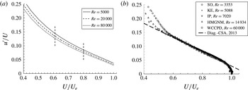
(a) Variation of axial turbulence intensity from (1.6) for the various $\mathit{Re}\equiv {\it\delta}^{+}={\it\delta}u_{{\it\tau}}/{\it\nu}$ , shown in the legend. The curves become lower as ${\it\delta}^{+}$ increases. Note that the total variation covers a factor of 16, with displacement thickness Reynolds numbers given by $\mathit{Re}_{{\it\delta}^{\ast }}$ increasing from about 16 000, through 67 000 to 270 000. The vertical dashed lines indicate the extent of the mean velocity log-law region at the highest $\mathit{Re}$ . (b) Turbulence intensity for a range of smooth-wall experimental and computational data; values of $\mathit{Re}$ are included in the legend for each data set, denoted by: SO, Schlatter & Örlü (Reference Schlatter and Örlü2010); KE, Krogstad & Efros (Reference Krogstad and Efros2012); IP, Inoue & Pullin (Reference Inoue and Pullin2011); HMGNM, Hutchins et al. (Reference Hutchins, Monty, Ganapathisubramani, Ng and Marusic2011); WCCPD, Winkel et al. (Reference Winkel, Cutbirth, Ceccio, Perlin and Dowling2012). The bold dashed line is the $u^{\prime }/U={\it\alpha}-{\it\beta}{\it\eta}$ relation from Castro et al. (Reference Castro, Segalini and Alfredsson2013).

The first thing to note about this plot is how slowly the curves shift (downwards) with increasing Reynolds number. A factor of 16 increase in ${\it\delta}^{+}$ leads to a fall of typically only 13 % in $u^{\prime }/U$ at $U/U_{e}=0.7$ (which we denote by $u^{\prime }/U|_{0.7}$ ). This factor (16) is roughly what is attainable in laboratory experiments on fully developed boundary layers (having constant value of the wake strength ${\it\Pi}$ ). Second, we point out that even at the highest Reynolds number, the range over which one expects the log-law to apply is limited to the region defined approximately by $0.61<U/U_{e}<0.80$ (using the upper and lower limits proposed by Marusic et al. Reference Marusic, Monty, Hultmark and Smits2013, i.e. $3\sqrt{{\it\delta}^{+}}<y^{+}<0.15{\it\delta}^{+}$ ). This range is indicated on the figure for the highest ${\it\delta}^{+}$ . Lower Reynolds numbers yield a more restricted log-law range. Currently, the highest ${\it\delta}^{+}$ laboratory data set available is that of Oweis et al. (Reference Oweis, Winkel, Cutbrith, Ceccio, Perlin and Dowling2010) (and Winkel et al. Reference Winkel, Cutbirth, Ceccio, Perlin and Dowling2012, for the corresponding stress data), at a momentum thickness Reynolds number $\mathit{Re}_{{\it\theta}}=156\,000$ . For this data ${\it\delta}^{+}$ is about 60 000, although the precise value depends on the definition of ${\it\delta}$ . Variations of, say, 25 % in this parameter would not noticeably shift the turbulence intensity curves (like those in figure 1).

Turbulence intensity data from various smooth-wall experiments, both laboratory and computational, are shown in figure 1(b). The data cover a range of nearly 18 in ${\it\delta}^{+}$ , from the direct numerical simulations (DNS) of Schlatter & Örlü (Reference Schlatter and Örlü2010) at ${\it\delta}^{+}=3353$ and the large-eddy simulations of Inoue & Pullin (Reference Inoue and Pullin2011) at ${\it\delta}^{+}=7020$ , to the laboratory data of Hutchins et al. (Reference Hutchins, Monty, Ganapathisubramani, Ng and Marusic2011), Krogstad & Efros (Reference Krogstad and Efros2012) and Winkel et al. (Reference Winkel, Cutbirth, Ceccio, Perlin and Dowling2012) at ${\it\delta}^{+}=5088$ , 14 934 and 60 000, respectively. These are all believed to be high-quality data sets for the canonical boundary layer. Note first that despite the wide range of ${\it\delta}^{+}$ the variation between the different sets of data, at least for $U/U_{e}>0.6$ , is noticeably smaller than the variations seen in figure 1(a). In fact, it is probably no more than the uncertainty in the data, whether from laboratory or numerical experiments. Second, the fits of each set of data to the straight-line relation (1.1) are, visually at least, no worse than they would be to the model curve (like those in figure 1 a) at the corresponding Reynolds number, particularly in the log-law region. Third, the fits to (1.1) actually extend over a considerably wider range than they would to the AEH model curve, with the extent increasing to lower $U/U_{e}$ as ${\it\delta}^{+}$ rises.

Recall that the AEH is really only formulated on the basis of assumptions made about the log-law region (e.g. that the turbulent shear stress is constant in that region, as Townsend Reference Townsend1976, postulated). Even if the assumptions were strictly valid (which they are not) one would not expect (1.6) to fit the data outside the log region. 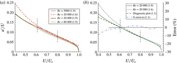The turbulence intensity behaviour arising from the more complete $U^{+}$ and $u^{\prime 2^{+}}$ profiles, i.e. (1.9), is shown in figure 2(a) for the same values of ${\it\delta}^{+}$ used in figure 1(a). For ${\it\delta}^{+}=20\,000$ the profile from (1.6) shown in figure 1(a) is included and it is clear that using the full composite profiles for $U^{+}$ and $u^{\prime 2^{+}}$ significantly straightens the $u^{\prime }/U$ versus $U/U_{e}$ plot on both sides of the log-law region. Figure 2(b) repeats the comparison and includes the diagnostic plot (1.1) and the percentage difference between the latter and what is deduced using the full composite profiles (1.9). The diagnostic plot differs from the behaviour expected using the full velocity and stress profiles by less than 3 % over the mean velocity range $0.48<U/U_{e}<0.96$ , which at this Reynolds number is equivalent to about $0.0037<y/{\it\delta}<0.61$ : a much wider range than the log-law range, both below and above the limits of the latter.

Figure 2.

(a) Variation of axial turbulence intensity for various $\mathit{Re}\equiv {\it\delta}^{+}={\it\delta}u_{{\it\tau}}/{\it\nu}$ , shown in the legend, using the full composite profiles (1.9) (from the combination of (1.7) and (1.8)). The dashed (red online) line is the simple (1.6) result, from figure 1(a). (b) The solid and dashed black curves are repeats of the $\mathit{Re}=20\,000$ data in figure 2(a). The heavy dashed linear (green online) line is the diagnostic plot (1.1) and the dash-dot (blue online) line shows the percentage error between this and the full result from (1.9). Both figures include the upper and lower limits of the log-law range (as in figure 1), indicated by the dashed vertical lines.

So what is in one sense curious about the data shown in figure 1(b) (and indeed all the very varied data sets that we have studied, see Castro et al. Reference Castro, Segalini and Alfredsson2013), in that they follow (1.1) well even though there seems no obvious physical basis for this behaviour, is in fact not so odd, since published composite profiles for both mean velocity and longitudinal stress imply a distribution of $u^{\prime }/U$ versus $U/U_{e}$ (i.e. (1.8) together with (1.7)) which is quite closely linear over a region of the boundary layer much wider than the extent of the usual log law, at least within some Reynolds number range. There is, nonetheless, a Reynolds number influence, as expected, and figure 2(a) suggests that at much lower Reynolds numbers the straight-line diagnostic plot behaviour will not work so well; the profile for ${\it\delta}^{+}=5000$ is clearly more curved through the buffer region between the log-law and linear very-near-wall regions.

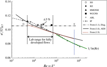
We can pursue further the matter of Reynolds number effects by considering data at a fixed value of $U/U_{e}$ compared with the expectations from (1.6), or indeed from the corresponding behaviour arising from use of the full composite profiles (1.9). Figure 3 compares this expectation for $U/U_{e}=0.7$ , along with the appropriate values from the data sets already mentioned. The figure shows the bounds within which all extant laboratory data fall (for cases where $\mathit{Re}_{{\it\theta}}$ is large enough to ensure a constant value of ${\it\Pi}$ ). Within this range, the model variation from either (1.6) or (1.9) is not very large; indeed, not much larger perhaps than experimental uncertainties; it is marginally smaller if the full model (1.9) is used. The figure includes results from the LES studies of Inoue & Pullin (Reference Inoue and Pullin2011) which actually extend up to $\mathit{Re}_{{\it\theta}}=10^{12}$ (i.e. very much farther than the largest ${\it\delta}^{+}$ shown). It is interesting that over the laboratory range these data are close to the (1.6) and (1.9) expectations and, indeed, the laboratory data, whereas at higher ${\it\delta}^{+}$ they fall below the expected trend. Note, however, that even for neutrally stable atmospheric boundary layers (ABLs), ${\it\delta}^{+}$ is typically $O(10^{6})$ and unlikely to be very much larger. The ABL data used by Marusic et al. (Reference Marusic, Monty, Hultmark and Smits2013) and originally reported by Hutchins et al. (Reference Hutchins, Chauhan, Marusic, Monty and Klewicki2012) has an estimated ${\it\delta}^{+}$ of 628 000 (indicated in figure 3), but because of the difficulty of assigning a proper boundary-layer depth, this is a somewhat crude estimate and it is difficult to estimate the proper $U_{e}$ . Nonetheless, using the best available estimate, the resulting $u^{\prime }/U^{\prime }|_{0.7}$ of about 0.108 is close to all of the results from the much lower ${\it\delta}^{+}$ (laboratory) data sets. (The definition of $U^{\prime }$ , used for rough-wall flows, is given in § 3, where the ABL data are discussed more fully.) Note also the one experimental data point at the highest laboratory ${\it\delta}^{+}$ yet achieved, using a large cavitation water channel (Winkel et al. Reference Winkel, Cutbirth, Ceccio, Perlin and Dowling2012). Like the ABL data point, this lies above the trend of the computed LES data, but is very similar to results from all of the other laboratory data. Collectively, all of the experimental data lie reasonably close to the expectation from the diagnostic plot (1.1), within the likely experimental error, whereas the LES data fall below both this and what would be expected from the AEH model (1.6) or its extension (1.9).

Figure 3.

The expected variation with ${\it\delta}^{+}$ of $U/U_{e}|_{0.7}$ from (1.6) (solid black line) and (1.9) (dotted (red online) line), compared with values from the various data sets, denoted in the legend by: SO, Schlatter & Örlü (Reference Schlatter and Örlü2010); KE, Krogstad & Efros (Reference Krogstad and Efros2012); IP, Inoue & Pullin (Reference Inoue and Pullin2011); HMGNM, Hutchins et al. (Reference Hutchins, Monty, Ganapathisubramani, Ng and Marusic2011); WCCPD, Winkel et al. (Reference Winkel, Cutbirth, Ceccio, Perlin and Dowling2012); AC, Amir & Castro (Reference Amir and Castro2011); ABL, Hutchins et al. (Reference Hutchins, Chauhan, Marusic, Monty and Klewicki2012). Solid symbols are from experiments, open symbols are from simulations. The solid (green online) line in the lower right of the figure is the asymptotic behaviour, $u^{\prime }/U\rightarrow f({\it\eta})/\ln ({\it\delta}^{+})$ (Pullin, Inoue & Salto Reference Pullin, Inoue and Salto2013). The vertical (blue online) dotted line indicates the estimated ${\it\delta}^{+}$ of the Hutchins et al. (Reference Hutchins, Chauhan, Marusic, Monty and Klewicki2012) ABL data.

What happens as ${\it\delta}^{+}\rightarrow \infty$ ? The data of Inoue & Pullin (Reference Inoue and Pullin2011), their subsequent asymptotics (Pullin et al. Reference Pullin, Inoue and Salto2013), and the AEH model relation (1.6) all suggest that as ${\it\delta}^{+}\rightarrow \infty$ , $u^{\prime }/U$ at any fixed $U/U_{e}$ tends to zero. Equation (1.6) implies that asymptotically, $u^{\prime }/U\rightarrow f({\it\eta})/\sqrt{\ln ({\it\delta}^{+})}$ whereas the analysis of Pullin et al. (Reference Pullin, Inoue and Salto2013) can be shown to imply $u^{\prime }/U\rightarrow f({\it\eta})/\!\ln ({\it\delta}^{+})$ , which is rather more rapid. Interestingly, the latter conforms quite well to the higher Reynolds number LES data of Inoue & Pullin (Reference Inoue and Pullin2011), as demonstrated in figure 3. In any case, it is clear that the fall in $u^{\prime }/U$ at fixed $U/U_{e}$ is a slow process; real flows of any scale surely never get anywhere near the final state of an essentially free-slip wall postulated by Pullin et al. (Reference Pullin, Inoue and Salto2013). From a practical perspective, the cases with much larger ${\it\delta}^{+}$ values than those shown in figure 3, computed by Inoue & Pullin (Reference Inoue and Pullin2011), are of little interest, certainly at planetary scales. Furthermore, it is worth noting that even their result for ${\it\delta}^{+}=1.1\times 10^{6}$ , shown in figure 3, refers to a location close to the grid point nearest to the wall, where the subgrid (and thus modelled) kinetic energy is about 70 % of the energy in all of the larger scales; the computed intensity might thus not be particularly accurate, and the situation must increasingly worsen for the higher-Reynolds-number simulations.

3. Rough-wall extensions

A rough surface leads to the addition of $-{\rm\Delta}U^{+}$ , the well-known roughness function, to the right-hand side of (1.2):

(3.1) $$\begin{eqnarray}U^{+}=\frac{1}{{\it\kappa}}\ln (y^{+})+A-{\rm\Delta}U^{+},\end{eqnarray}$$

which leads to a more general version of (1.4), namely

(3.2) $$\begin{eqnarray}u^{\prime 2^{+}}=C-A_{1}({\it\kappa}U^{+}+{\rm\Delta}U^{+})\end{eqnarray}$$

and thus a similarly more-general version of (1.6), which can be written

(3.3) $$\begin{eqnarray}u^{\prime }/U^{\prime }=\frac{(D-E{\it\eta}^{\prime }(1+{\rm\Delta}U_{n}))^{1/2}}{{\it\eta}^{\prime }},\end{eqnarray}$$

where now the scaling mean velocity is $U^{\prime }=U+{\rm\Delta}U$ , the normalised mean velocity parameter is ${\it\eta}^{\prime }=(U+{\rm\Delta}U)/(U_{e}+{\rm\Delta}U)$ and ${\rm\Delta}U_{n}={\rm\Delta}U/U_{e}$ . Both $U^{\prime }$ and ${\it\eta}^{\prime }$ revert of course to the smooth-wall equivalents for ${\rm\Delta}U=0$ . (A similar modification would be necessary for the composite profile result, (1.9).) Castro et al. (Reference Castro, Segalini and Alfredsson2013) discussed this more generalised scaling and demonstrated that ${\rm\Delta}U_{n}$ does not exceed an $O(1)$ quantity for rough surfaces (even in a very rough ABL such as that over cities). The ‘constants’ in (3.3) ( $C,D,E$ ) were defined in § 1 but now, for a given ${\it\delta}^{+}$ and ${\rm\Delta}U_{n}$ , $C_{f}/2$ (in $D$ and $E$ ) is determined from the more general version of (2.2), i.e.

(3.4) $$\begin{eqnarray}U_{e}^{+}=\left.\left(\frac{1}{{\it\kappa}}\ln ({\it\delta}^{+})+A+2{\it\Pi}/{\it\kappa}\right)\right/(1+{\rm\Delta}U_{n}),\end{eqnarray}$$

with the universality assumption that ${\it\kappa}$ , $A$ and ${\it\Pi}$ are identical to their smooth-wall values. Equation (3.3) may be compared with the more general version of (1.1),

(3.5) $$\begin{eqnarray}\frac{u^{\prime }}{U^{\prime }}={\it\alpha}-{\it\beta}{\it\eta}^{\prime },\end{eqnarray}$$

or the corresponding rough-wall extension of the full relation (1.9), which merely contains the extra $-{\rm\Delta}U^{+}$ in the expression for $U_{c}^{+}$ . Castro et al. (Reference Castro, Segalini and Alfredsson2013) also showed that extant rough-wall data fit this latter expression (with the same values of ${\it\alpha}$ and ${\it\beta}$ as for smooth flows), independent of Reynolds number. Not surprisingly perhaps, the curve defined by (3.3) for a particular ${\it\delta}^{+}$ collapses on to that of (1.6) for the same ${\it\delta}^{+}$ (and ${\rm\Delta}U=0$ ). However, the ${\it\eta}^{\prime }$ range covered is smaller so that, taking ${\it\delta}^{+}=10\,000$ and ${\rm\Delta}U_{n}=1$ as an example case, the value of ${\it\eta}^{\prime }$ corresponding to ${\it\eta}=0.4$ is 0.7. In principle, if it were possible that ${\rm\Delta}U_{n}\rightarrow \infty$ , the curve of $u^{\prime }/U^{\prime }$ versus ${\it\eta}^{\prime }$ would collapse to a point at $(1,0)$ but, as mentioned above, ${\rm\Delta}U_{n}$ does not normally exceed  $O(1)$ .

Figure 4.

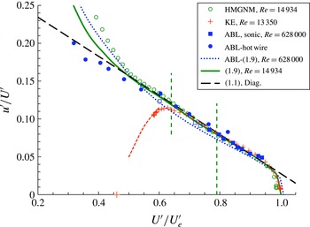
Data from Hutchins et al. (Reference Hutchins, Monty, Ganapathisubramani, Ng and Marusic2011) (HMGNM, smooth wall), Krogstad & Efros (Reference Krogstad and Efros2012) (KE, rough wall), and Hutchins et al. (Reference Hutchins, Chauhan, Marusic, Monty and Klewicki2012) (ABL, rough surface) compared with the full model (1.9). The vertical dashed lines indicate the extent of the log-law region for the Hutchins et al. (Reference Hutchins, Monty, Ganapathisubramani, Ng and Marusic2011) flow. The (red online) cross at $u^{\prime }/U^{\prime }=0$ is the value of $U^{\prime }/U_{e}^{\prime }$ (0.46) when $U=0$ for the Krogstad & Efros (Reference Krogstad and Efros2012) profile.

The major point is that surface roughness does not change the expected behaviour of the outer layer turbulence intensity as predicted by the AEH, which is in accord with the classical Townsend hypothesis. Furthermore, rough-wall data, whether from laboratory or numerical experiments, collapse onto the same diagnostic plot, as shown by Castro et al. (Reference Castro, Segalini and Alfredsson2013). As an example, figure 4, which again shows the smooth-wall Hutchins et al. (Reference Hutchins, Monty, Ganapathisubramani, Ng and Marusic2011) data for ${\it\delta}^{+}\approx 15\,000$ (the highest ${\it\delta}^{+}$ case currently available from wind tunnel smooth-wall experiments), also shows the data from Krogstad & Efros (Reference Krogstad and Efros2012) which are for a flow at ${\it\delta}^{+}=13\,350$ over two-dimensional bar roughness (for which ${\rm\Delta}U_{n}=0.82$ ). Since the flow has a very similar ${\it\delta}^{+}$ to that of the Hutchins et al. (Reference Hutchins, Monty, Ganapathisubramani, Ng and Marusic2011) smooth-wall flow the notional log-law limits are practically the same and it is evident that the data scaled this way collapse to both (3.5) and (1.9) quite well in both the log-law region and, beyond that, well into both the buffer layer and the outer (wake) part of the flow. Incidentally, the fit in the buffer region (for smooth-wall cases) is quite sensitive to the specific values of $A_{1}$ and $B_{1}$ ; small changes in these, for example as evident in the papers of Marusic et al. (Reference Marusic, Uddin and Perry1997) and Chauhan et al. (Reference Chauhan, Monkwitz and Nagib2009), lead to significant shifts in that part of the profile. We have used the values given by the former, but those authors also used ‘older’ values of $A$ and ${\it\kappa}$ (5.0 and 0.41, respectively) in the mean flow profile; strictly, that ( $A$ , ${\it\kappa}$ ) pair would require adjustments to the other constants in Chauhan’s composite mean flow profile but this has not been pursued here.

The rough-wall case highlights the inability (not surprisingly) of the AEH model to describe the behaviour near the wall. In such cases the lowest possible value of $U^{\prime }/U_{e}^{\prime }$ (when $U=0$ ) is ${\rm\Delta}U_{n}/(1+{\rm\Delta}U_{n})$ and, despite the complications very close to and within the roughness, $u^{\prime }$ must be zero at that location; this point is shown in figure 4 for the value of ${\rm\Delta}U_{n}$ appropriate to the Krogstad & Efros (Reference Krogstad and Efros2012) flow and the measured data have already begun to fall towards this point. The peak in $u^{\prime }/U^{\prime }$ for this flow is around 0.11, corresponding to a turbulence intensity of $u^{\prime }/U\approx 0.47$ which is significantly higher than the near-wall asymptote for smooth walls (around 0.4). Smooth-wall data also have a peak (or two) in the normal stresses, but these lie well below the bottom $U/U_{e}$ extent of the axis in this figure; naturally, the AEH ceases to apply around, and below, that height, where viscous effects become significant. Rough-wall boundary layers always contain a roughness sublayer which must extend some distance above the top of the roughness and within which the flow is inhomogeneous in spanwise planes. The form taken by mean velocity and stress profiles within this region depends on the roughness morphology and the specific location of the profile, but there is no doubt that the roughness sublayer can severely restrict the lower extent of the log-law region, effectively ‘squeezing’ this region from below. The (outer) peak in $u^{\prime }/U^{\prime }$ usually occurs just outside the roughness sublayer; in the Krogstad & Efros (Reference Krogstad and Efros2012) case it occurs at a height of about $3h$ , where $h$ is the height of the roughness, but a good fit of the mean velocity to the log law extends down to around $2h$ .

In the very first paper proposing the diagnostic plot, Alfredsson & Örlü (Reference Alfredsson and Örlü2010) noted the possibility that ‘if the Reynolds number variation is small in the outer region the diagnostic plot may be used to estimate the boundary layer free stream velocity … which may be helpful when studying the ABL’. But they noted later that ABL data may be affected by surface roughness (Alfredsson et al. Reference Alfredsson, Örlü and Segalini2012); this makes any proposed comparisons with either the diagnostic plot (3.5) or the implications of the AEH (3.3) even more difficult. We noted earlier that in experiments within the ABL it is impossible to be certain about either the precise boundary-layer depth (and, hence, ${\it\delta}^{+}$ ) or the effective $U_{e}$ , let alone ${\rm\Delta}U$ . However, with an estimate of the surface roughness, some progress is possible. The ABL data included in figure 4 are from the experiments described by Hutchins et al. (Reference Hutchins, Chauhan, Marusic, Monty and Klewicki2012), who estimated the appropriate boundary-layer depth to be about 60 m, giving a Reynolds number of ${\it\delta}^{+}=628\,000$ . They stated that ${\it\delta}$ is ‘roughly estimated based on radiosonde measurements that determine the edge of the logarithmic region’ (Metzger, McKeon & Holmes Reference Metzger, McKeon and Holmes2007). An appropriate $U_{e}^{+}$ is therefore the value of $U^{+}$ at that point, which for the Hutchins et al. (Reference Hutchins, Chauhan, Marusic, Monty and Klewicki2012) data would be about 37.3. All of the authors who have studied the flow at that site in Utah have recognised that the surface is transitionally rough and Hutchins et al. (Reference Hutchins, Chauhan, Marusic, Monty and Klewicki2012) provided an estimated equivalent sand-grain roughness, $k_{s}^{+}$ , of about 21, which is equivalent to ${\rm\Delta}U^{+}=3.6$ using the standard Schlichting (Reference Schlichting1968) relation. These values imply ${\rm\Delta}U_{n}\equiv {\rm\Delta}U^{+}/U_{e}^{+}=0.097$ and this enables the data to be presented in the form of $u^{\prime }/U^{\prime }$ versus $U^{\prime }/U_{e}^{\prime }$ . Figure 4 includes the resulting profile. If one were to accept the AEH model for this flow, one can use (1.9) (with roughness function included) to deduce the expected $u^{\prime }/U^{\prime }$ curve; this is included in figure 4 and lies somewhat below the curve appropriate to the data of Hutchins et al. (Reference Hutchins, Monty, Ganapathisubramani, Ng and Marusic2011) (since the Reynolds number is more than 40 times higher), and also below the measured data. Accepting that the $k_{s}^{+}$ and ${\it\delta}^{+}$ values suggested by Hutchins et al. (Reference Hutchins, Chauhan, Marusic, Monty and Klewicki2012) (with the implied value of $U_{e}^{+}$ ) are not unreasonable, it is striking that the data lie close to the diagnostic (3.5) relation and remain well-fitted by this over a very wide range of $U/U_{e}$ . Nonetheless, it must be admitted that given the uncertainties in ABL parameters it would perhaps not be wise to draw too much from this comparison. Interestingly, the height of the lowest measured $U/U_{e}$ value shown in figure 4 was about 2 mm from the desert surface, which is probably within the roughness sublayer since it is about the same as the average height of the surface excrescences quoted by Metzger et al. (Reference Metzger, McKeon and Holmes2007).

There are some circumstances in which a surface may be sufficiently rough and have a sufficiently small-scale separation (characterised loosely by the ratio of ${\it\delta}$ and the roughness height $k$ ) that very little log-law can be expected. In such cases it can be very difficult to estimate $C_{f}$ (and, hence, $U_{e}^{+}$ ) from mean flow or turbulence measurements. But if the diagnostic plot is assumed to provide a good fit to the intensity data one can deduce ${\rm\Delta}U_{n}$ by choosing the value that provides the best fit between the data and (3.5) and then estimate $U_{e}^{+}$ by adjusting it to yield a ${\rm\Delta}U^{+}$ which gives a satisfactory trend of the data towards the log-law line (3.1). If $C_{f}$ were available from an independent drag measurement (e.g. from a drag balance), this would give some confidence, or otherwise, in this estimated $U_{e}^{+}$ . However, one must bear in mind that such flows are probably quite far from having classical boundary-layer characteristics and the turbulence intensity profile may thus not necessarily be expected to conform to either (3.3) or (3.5).

4. Channel flow extensions

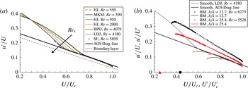
Alfredsson et al. (Reference Alfredsson, Örlü and Segalini2012) demonstrated that the diagnostic plot relation expressed by (1.1) was also well-fitted by smooth-wall channel (and pipe) flow data, albeit with slightly different values of the constants ( ${\it\alpha}=0.314$ , ${\it\beta}=0.267$ ) largely because of the non-zero value of $u^{\prime }$ on the channel centreline. Again, the range of the linear fit was shown to increase with Reynolds number. Figure 5(a) shows a typical plot and includes more recent DNS and laboratory data at significantly higher Reynolds numbers than the data available to Alfredsson et al. (Reference Alfredsson, Örlü and Segalini2012). Note the very clear trend with increasing $\mathit{Re}$ ( $\equiv hu_{{\it\tau}}/{\it\nu}$ where $h$ is the channel half-height), particularly the increasing extent of the outer layer behaviour; once $\mathit{Re}$ exceeds about 4000, the linear fit extends for all $U/U_{c}>0.6$ , where $U_{c}$ is the channel centreline velocity.

Figure 5.

(a) Smooth-wall DNS channel data from Moser, Kim & Mansour (Reference Moser, Kim and Mansour1999) (MKM in legend), Hoyas & Jiménez (Reference Hoyas and Jiménez2006) (HJ), Bernardini, Pirozzoli & Orlandi (Reference Bernardini, Pirozzoli and Orlandi2014) (BP), Lozano-Durán & Jiménez (Reference Lozano-Durán and Jiménez2014) (LDJ) and Laser Doppler data from Schultz & Flack (Reference Schultz and Flack2013) (SF). Legend shows author initials, year and $\mathit{Re}\equiv hu_{{\it\tau}}/{\it\nu}$ . The dashed straight line is the diagnostic relation for the boundary layer and the solid (red online) line is the channel relation given by Alfredsson et al. (Reference Alfredsson, Örlü and Segalini2012). (b) Two sets of rough-wall channel data from Birch & Morrison (Reference Birch and Morrison2011). The legend shows the ratio of channel half-height to roughness height (i.e.  $h/k$ ) and $\mathit{Re}$ . Small symbols are the $u^{\prime }/U$ versus $U/U_{c}$ data and corresponding lines show the data scaled using $U+{\rm\Delta}U$ (i.e.  $u^{\prime }/U^{\prime }$ versus $U^{\prime }/U_{c}^{\prime }$ ). Large open symbols mark $u^{\prime }/U^{\prime },U^{\prime }/U_{c}^{\prime }$ at the points where $y=2.5k$ in the two profiles. Large solid symbols show the $U^{\prime }/U_{c}^{\prime }$ values where $U=0$ in the two cases. The high- $\mathit{Re}$ smooth-wall profile of Lozano-Durán & Jiménez (Reference Lozano-Durán and Jiménez2014) is included.

Given the appropriate value of the roughness function and using the resulting adjusted scaling ( $U^{\prime }=U+{\rm\Delta}U$ , etc.), we expect rough-wall outer-layer profiles to collapse onto the smooth wall result provided there is sufficient scale separation, roughly characterised by $h/k$ . (Note that a more precise characterisation of scale separation is provided by $h/y_{o}$ , where $y_{o}$ is the roughness length of the surface, as discussed in the context of boundary layers by Castro et al. Reference Castro, Segalini and Alfredsson2013.) Figure 5(b) shows data from Birch & Morrison (Reference Birch and Morrison2011) for expanded mesh and grit roughnesses, height $k$ , having $h/k\approx 12.7$ and 25.4, respectively. In both cases the surface is fully rough. It is evident that, as in the case of boundary layers, $u^{\prime }/U$ versus $U/U_{c}$ profiles are closely linear but with slopes greater than the smooth wall slope, whereas including the appropriate ${\rm\Delta}U$ in the mean velocity terms (i.e. plotting $u^{\prime }/U^{\prime }$ versus $U^{\prime }/U_{c}^{\prime }$ ) leads to good collapse almost everywhere above about two-and-a-half times the roughness height (which is roughly the upper limit of the roughness sublayer and is indicated on the figure). Below that, the data fall off below the straight line and begin the trend towards the $u^{\prime }=0$ points marked on the $U^{\prime }/U_{c}^{\prime }$ axis, but the profiles there depend on precisely where they are measured. For reference, details of the four rough-wall data sets used (in §§ 3 and 4) are given in table 1.

Table 1.

Summary of rough wall data sets. Note that the ABL flow is almost certainly transitionally rough. All other data in the paper are for smooth wall flows, for which $\mathit{Re}_{{\it\tau}}$ is the only relevant parameter.

5. Free shear layer extensions

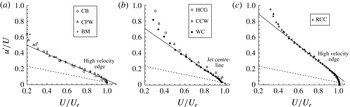
Given the good fit of the linear diagnostic plot to both smooth- and rough-wall boundary layers and channels, the apparently very weak Reynolds number dependence (for fully developed flows), and the lack of any dependence on wall location or wall stress in (1.1), it is tempting to consider whether (1.1) might be followed in shear flows remote from any walls. We consider the three major types of free shear flows: jets, wakes and mixing layers. Figure 6 shows data extracted from samples of the published literature for all three flow types. The sample flows were chosen on the basis simply of both ease of accessibility and sufficiently detailed data. We briefly consider each of the three flow types in turn.

Figure 6.

Diagnostic plots for (a) the plane mixing layer; (b) axisymmetric and planar jets; (c) axisymmetric wakes. (a) CB is Castro & Bradshaw (Reference Castro and Bradshaw1976), CPW is Champagne, Pao & Wygnanski (Reference Champagne, Pao and Wygnanski1976), BM is Bell & Mehta (Reference Bell and Mehta1990). (b) HCG is Hussain, Capp & George (Reference Hussain, Capp and George1994) (round jet), CCW is Cant, Castro & Walklate (Reference Cant, Castro and Walklate2002) (plane jet), WC is Webb & Castro (Reference Webb and Castro2006) (round jet). (c) RCC is Redford, Castro & Coleman (Reference Redford, Castro and Coleman2012). The dashed line in each case is (1.1) with the boundary layer values of ${\it\alpha}$ and ${\it\beta}$ ; solid lines show reasonable straight line fits to the data.

Two of the three planar mixing layers cases shown in figure 6(a) (those of Castro & Bradshaw Reference Castro and Bradshaw1976; Champagne et al. Reference Champagne, Pao and Wygnanski1976) have ambient (nominally zero-velocity) air on one side and there the turbulence intensities thus become very large. The third case (Bell & Mehta Reference Bell and Mehta1990) is a layer between two (non-zero velocity) streams but also naturally has the largest intensities on the low-speed side of the layer. The velocity $U_{e}$ is the velocity on the high-speed side of the layers and it is clear that once $U/U_{e}$ exceeds about 0.4 there is a reasonably good collapse to a linear relationship like (1.1), albeit with a significantly higher slope ( ${\it\beta}$ ) than that for boundary layers.

It is less obvious how to scale the data from jets since in such flows the smallest turbulence intensities do not occur at the edges (where the mean velocity is zero) but in the centre, where the mean velocity has its maximum. And even there, on the centreline in particular, the intensity is obviously not zero. An appropriate reference mean velocity in this case is the maximum jet velocity, with local velocities ( $U$ ) defined as the variation from this value. Likewise, for wake flows, the scaling $U_{e}$ is taken as the maximum velocity deficit, with local mean velocities taken as the local deficit. In both the jet and wake cases data are shown for the region of the flow from a location roughly where turbulence production is a maximum (i.e. where, approximately, the turbulent shear stress is a maximum) to the point where the turbulence intensities fall closest to zero. The jet flow data in figure 6(b) are from both planar (Cant et al. Reference Cant, Castro and Walklate2002) and axisymmetric (Hussain et al. Reference Hussain, Capp and George1994; Webb & Castro Reference Webb and Castro2006) cases, whereas the wake flow data in figure 6(c) are from the recent DNS of a time-developing axisymmetric case (Redford et al. Reference Redford, Castro and Coleman2012). Note again that the data all conform reasonably to (1.1).

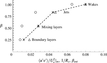
It is interesting and surely significant that the slope of the linear fits increases through the flow sequence, i.e. from boundary layers, through mixing layers and jets, to wakes. At the very least, this is a reflection of the increasing values of the maximum Reynolds shear stress normalised using the reference mean velocity, which is (typically) about 0.008 in a zero-pressure-gradient boundary layer (at ${\it\delta}^{+}\approx 60\,000$ ) and 0.01, 0.025 and 0.065 in mixing layers, jets and wakes, respectively. This follows the trend through these different flows of decreasing total mean strain rate and in particular the ‘flow constant’, $R_{s}$ , as discussed originally by Townsend (Reference Townsend1976), where $R_{s}$ is effectively a Reynolds number characteristic of the particular type of flow and defined using the scaling mean velocity $U_{e}$ , a suitable flow width, and the eddy viscosity. Here $R_{s}$ is inversely proportional to the entrainment parameter as defined by Townsend. The increasing value of ${\it\beta}$ through the different flow types thus follows an increasing value of the entrainment parameter, which is here termed ${\it\beta}_{ent}$ . Figure 7 shows the variation of the slope ${\it\beta}$ of the diagnostic plot with the maximum shear stress, $1/R_{s}$ and ${\it\beta}_{ent}$ for the different flow types. The particular values of these latter three parameters have been taken from Townsend (Reference Townsend1976), but more recent data would not change them significantly. The figure emphasises the monotonic (though not linear) variation of ${\it\beta}$ through the different flow types. It is perhaps little surprise that the rate at which local turbulence intensities fall as the free stream is approached increases with the entrainment velocity (which Townsend showed increases roughly proportionally to the increase in ${\it\beta}_{ent}$ ).

Figure 7.

Slope of the diagnostic plot ( ${\it\beta}$ ) versus the maximum shear stress (○, $\overline{u^{\prime }v^{\prime }}/U_{e}^{2}|_{m}$ ), the inverse of Townsend’s flow constant (▵, $1/R_{s}$ ) and Townsend’s entrainment parameter ( $\times$ , ${\it\beta}_{ent}$ ), for the four different classical flow types.

The main point about figure 6 in the present context, however, is that for all of these classical (roughly self-preserving) flows $u^{\prime }/U$ falls linearly with increasing $U/U_{e}$ once $U/U_{e}>0.5$ (say). Normalising $u^{\prime }/U$ by its value near the region of maximum kinetic energy production (i.e. where $-\overline{u^{\prime }v^{\prime }}\partial U/\partial y$ is a maximum) leads to a reasonable collapse of all of the data from all of the flows onto a single line, but this adds little of significance to the ‘raw’ results shown in figure 6.