


Introduction
Climate change is increasingly recognised as a major driver of ecological disruption, particularly in the agricultural sector (EPPO (European and Mediterranean Plant Protection Organization), 2022; Yang et al., Reference Yang, Tilman, Jin, Smith, Barrett, Zhu, Burney, D’Odorico, Fantke, Fargione and Finlay2024). For insect pests, climate change may lead to changes in their distribution, altered overwintering survival, increased numbers of generations per year, or disrupted synchronisation with host plants (Song et al., Reference Song, Li, Gao, Yan, Zhang, Liu and Zhou2024; Ullah et al., Reference Ullah, Abbas and Gul2024). Climate change also alters interspecific interactions, heightens invasion risks, increases the incidence of insect-transmitted diseases, and reduces the impact of biological control strategies (Abbas et al., Reference Abbas, Ullah, Hafeez, Han, Dara, Gul and Zhao2022; Ullah et al., Reference Ullah, Abbas and Gul2024). These changes collectively exacerbate crop damage and cause substantial economic losses worldwide (Bellard et al., Reference Bellard, Bertelsmeier, Leadley, Thuiller and Courchamp2012; Deutsch et al., Reference Deutsch, Tewksbury, Tigchelaar, Battisti, Merrill, Huey and Naylor2018; FAO (Food and Agriculture Organization), 2021). Studies of changes in species distribution under shifting climate conditions can provide economically effective conservation measures and prevent imbalances in ecological systems (Urban, Reference Urban2017; Sun et al., Reference Sun, Wang, Zhou, Wang, Wang, Lyu and Li2020; Qiao et al., Reference Qiao, Zhuang, Wang, Xie, Zhang, Shen and Zhou2025).
The planthopper Oecleopsis sinicus (Jacobi, 1944) (Hemiptera, Fulgoromorpha, Cixiidae) was originally recorded from the provinces of Hunan, Guangxi, and Fujian in China. Currently, this species has spread to Shaanxi, Anhui, Henan, Sichuan, Guizhou, Guangdong, Zhejiang, Hubei, and Beijing. It has also been recorded from Japan (Kyushu) and Cambodia (Guo et al., Reference Guo, Wang and Feng2009; Kawahara et al., Reference Kawahara, Ohshima and Matsumoto2011; Hayashi and Fujinuma, Reference Hayashi and Fujinuma2016; Zhi et al., Reference Zhi, Huang, Chen, Pan and Zhang2018; Luo et al., Reference Luo, Yang, Peng, Xie, Song and Zhang2022; Lv et al., Reference Lv, Dong, Chen, Geng and Jiang2024). This species causes significant crop damage through phloem feeding and virus transmission. For example, in Guangdong, outbreaks of this pest reduced rice yield by 1.7 t ha−1 (from 8.1 to 6.4 t ha−1) causing economic losses of approximately 15,000 CNY ha−1 (approximately US $2,100 ha−1) (Luo et al., Reference Luo, Yang, Peng, Xie, Song and Zhang2022); in Japan (2016), O. sinicus transmitted rice black-streaked dwarf virus, resulting in 25% yield losses across 1,200 ha and damage valued at 420 million JPY (Kawahara et al., Reference Kawahara, Ohshima and Matsumoto2011).
Since the first description of O. sinicus by Jacobi in 1944, global temperatures have risen by more than 1.1–1.5°C, with accelerated warming since 1940 (NASA Earth Science Division, 2025), the recent expansion of O. sinicus is likely due to warming. Therefore, we employ the MaxEnt model to project the distribution range of O. sinicus across Asia. The potential future distribution area of O. sinicus across other Asian countries is also studied using the MaxEnt model, which provides important information for predicting the species’ regional dispersal patterns and facilitating effective pest management strategies throughout Asia.
Materials and methods
Methodological approach for species distribution modelling (SDM)
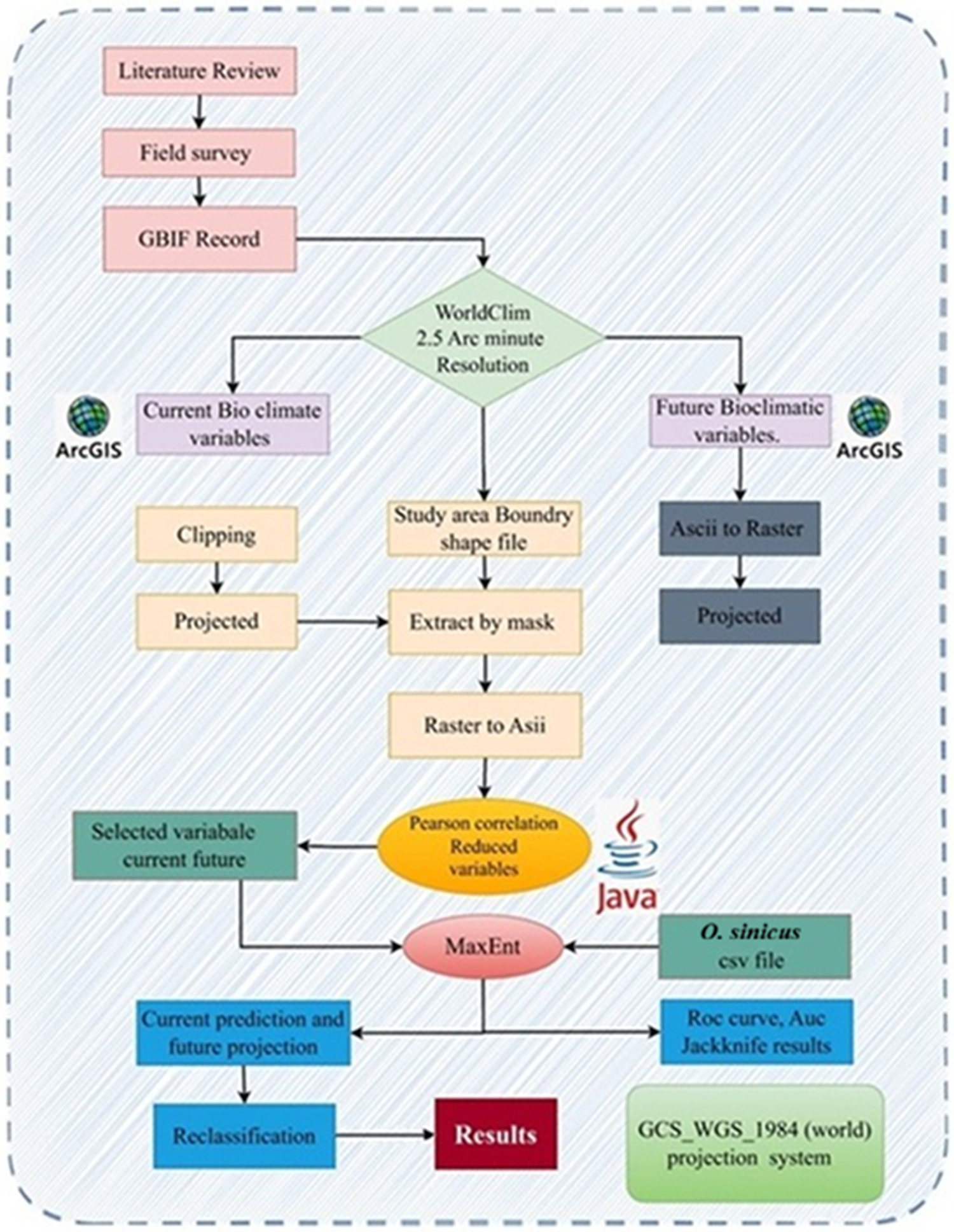
In this study, a detailed methodological framework was used to predict the distribution of O. sinicus in accordance with the established protocols by Chan et al. (Reference Chan, Leow, Bea, Cheng, Phoong, Hong and Chen2022), Liu et al. (Reference Liu, Zheng, Guan, Han and Liu2023), and Xue et al. (Reference Xue, Shahbaz, Ahmed, Ahmad and Sinha2022). The workflow included sequential processes, from initial data collection to final habitat suitability predictions, such as species occurrence data acquisition and geographic record processing and validation, selection of bioclimatic variables, MaxEnt model development, and classification of habitats under current and future climatic conditions. Figure 1 shows an advanced workflow diagram for this methodological approach.
Methods adopted to predict the distribution of O. sinicus.

Figure 1 Long description
The flowchart begins with three initial steps: Literature Review, Field Survey and GBIF Record. These steps lead to WorldClim with a resolution of 2.5 arc minutes. From WorldClim, two paths diverge: Current Bioclimatic Variables and Future Bioclimatic Variables, both utilizing ArcGIS. The Current Bioclimatic Variables path involves Clipping and Projected processes, while the Future Bioclimatic Variables path involves Ascii to Raster and Projected processes. Both paths converge at the Study Area Boundary Shape File, which is processed by Extract by Mask and Raster to Ascii. The next step involves Pearson Correlation and Reduced Variables, facilitated by Java. This leads to MaxEnt, which uses Selected Variable Current Future and O. sinicus CSV file. The MaxEnt process results in Current Prediction and Future Projection, followed by Reclassification. The final output is labeled as Results, using the GCSWGS1984 (world) projection system.
Species distribution data collection
Data on species occurrence records were collected from three sources: (1) the Centre for Agriculture and Bioscience International (CABI, https://www.cabi.org/ on 25 February 2025); (2) the Global Biodiversity Information Facility database (GBIF, https://www.gbif.org/ (accessed on 11 April 2025)); and (3) published literature (Guo et al., Reference Guo, Wang and Feng2009; Kawahara et al., Reference Kawahara, Ohshima and Matsumoto2011; Zhi et al., Reference Zhi, Huang, Chen, Pan and Zhang2018; Luo et al., Reference Luo, Yang, Peng, Xie, Song and Zhang2022; Lv et al., Reference Lv, Dong, Chen, Geng and Jiang2024). The total number of occurrence records received by this method was 216 localities. Google Earth was used to convert all the locations into geocoordinates (http://ditu.google.cn/ accessed on 15 April 2025).
Geographic record processing and validation
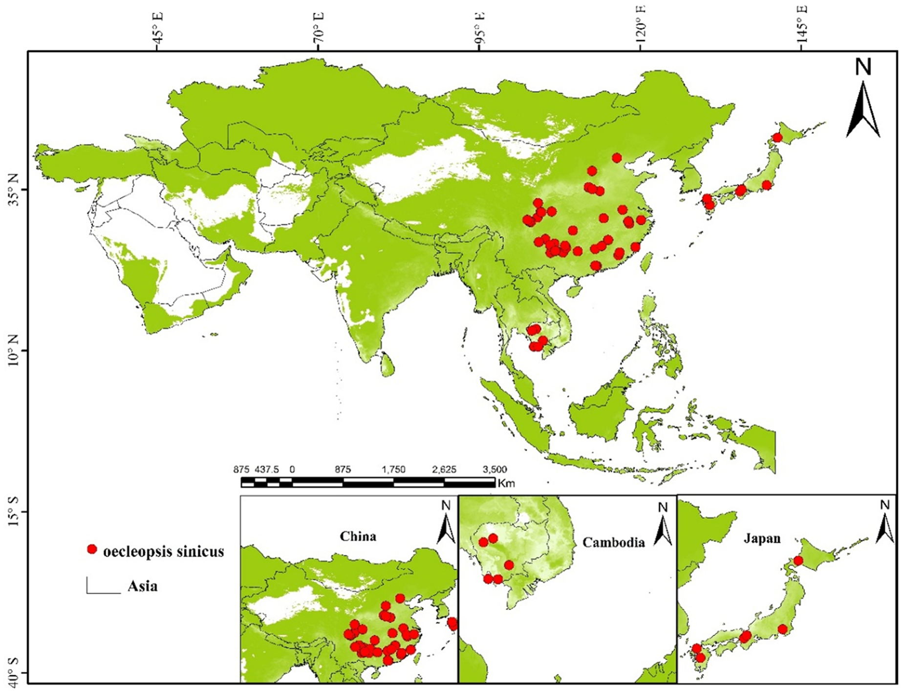
The data on distribution were processed as follows: (1) remove the distributions without coordinates, the distributions with zero coordinates, and the duplicates; and (2) the software CoordinateCleaner 3.0.1 was utilised. Spatial filtering was used to verify that every grid cell had a single allocation site, at a resolution of 2.5 arc minutes, with a single distribution point at following the filtering process, we gathered 209 distribution records, which were subsequently mapped onto an Asian map using ArcGIS 10.8.2 (http://www.arcgis.com/) (fig. 2). The shapefile delineating Asia’s boundary was sourced from the ‘Resource and Environmental Science Data Platform’ website (https://www.resdc.cn/, accessed 12 March 2025).
Occurrence records of Oecleopsis sinicus.

Figure 2 Long description
The map displays the distribution of Oecleopsis sinicus across Asia, marked by red dots. The main map shows clusters of distribution points in eastern China, Japan and parts of Southeast Asia. Insets provide detailed views of specific regions: China, Cambodia and Japan. In China, the distribution is concentrated in the eastern and southeastern areas. In Cambodia, the points are scattered across the country. In Japan, the distribution is primarily along the main islands. The map includes a scale bar indicating distances in kilometers and directional arrows for orientation. The legend identifies the red dots as locations of Oecleopsis sinicus and outlines the boundary of Asia.
Bioclimatic variables and future climate data projections
The average, minimum, and maximum temperature and precipitation data from 1970 to 2000 were represented by 19 bioclimatic variables that were downloaded at a 2.5 arc-minute geographical resolution from WorldClim (http://www.worldclim.org/download, accessed 20 January 2025) (table S1). In conjunction with future climate prediction data, are utilised to assess how climate change affects the distribution of species.
The future climate data are long-term climatological averages for three periods: 2041–2060, 2061–2080, and 2081–2100. These projections were derived from the BCC-CSM2-MR global climate model (GCM) under four Shared Socioeconomic Pathway (SSP) scenarios: SSP126, SSP245, SSP370, and SSP585. In this study, the BCC-CSM2-MR GCM was selected exclusively for its suitability to the designated study area. The analysis incorporated all combinations of two scenarios (SSP126 and SSP585), resulting in four distinct climate-change scenarios. ArcGIS software (version 10.8.2) was used to process data for the Asian study area.
Variable selection
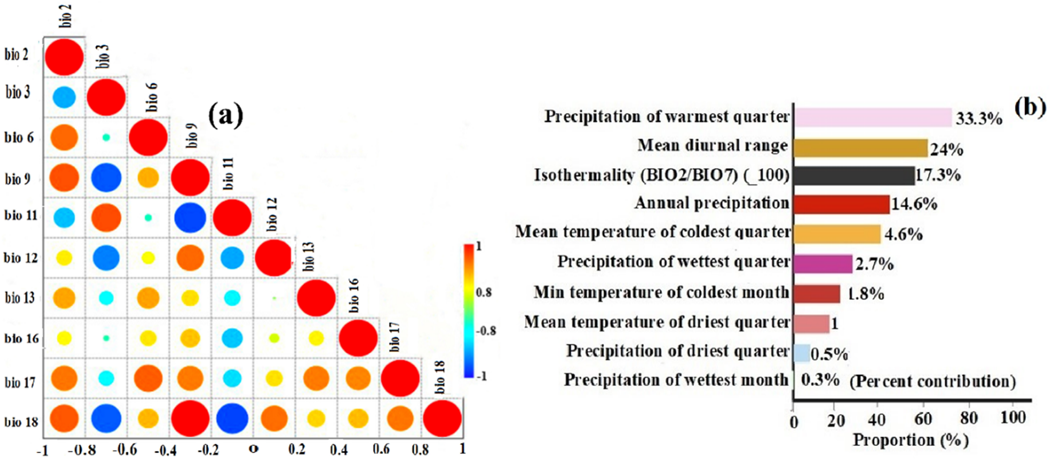
To eliminate multicollinearity bias, Pearson correlation coefficients (r) between the variables were computed for 1970–2000 using the ENM tool (fig. 3a and table S1). When the Pearson correlation exceeded 0.85, one of the two variables was eliminated based on the current understanding of species ecology worldwide.
(a) Analysis of Pearson correlation. Note: The value of correlation coefficient is shown on the horizontal axis. (b) Major climatic factors.

Figure 3 Long description
The image A showing a triangular correlation matrix with circular markers in each cell. A vertical scale at the right side is labeled from 0 to 1 with tick labels 0, 0.2, 0.4, 0.6, 0.8, 1. The matrix has variable labels along the left side and along the diagonal, including bio 2, bio 3, bio 6, bio 9, bio 11, bio 12, bio 13, bio 14, bio 15, bio 16, bio 17, bio 18. The bottom axis shows correlation coefficient tick labels: negative 0.8, negative 0.6, negative 0.4, negative 0.2, 0, 0.2, 0.4, 0.6, 0.8. The circles vary in size across cells. The image B showing a horizontal bar chart listing climatic variables on the vertical axis and proportions on the horizontal axis. The horizontal axis label reads Proportion percent, with tick labels 0, 20, 40, 60, 80, 100. The vertical axis lists: Precipitation of warmest quarter, Mean diurnal range, Isothermality (bio 2 over bio 7) times 100, Annual precipitation, Mean temperature of coldest quarter, Precipitation of wettest quarter, Min temperature of coldest month, Mean temperature of driest quarter, Precipitation of driest quarter, Precipitation of wettest month. Percentage values shown at the ends of the bars are: 33.3 percent, 24 percent, 17.3 percent, 14.6 percent, 4.6 percent, 2.7 percent, 1.8 percent, 1 percent, 0.5 percent, 0.2 percent.
Only ten environmental variables (BIO2, BIO3, BIO6, BIO9, BIO11, BIO12, BIO13, BIO16, BIO17, and BIO18) for O. sinicus were employed in the modelling following these eliminations (fig. 3b and table S1). All factors were included in SDM studies, and the jackknife test was used to assess each variable’s contribution to the model (table S1). The distribution of O. sinicus is most influenced by factors such as annual rainfall, the average temperature during the coldest quarter, the precipitation in the driest month, and temperature variability. The three resampling techniques available in MaxEnt software are bootstrapping, cross-validation, and subsampling. These techniques produce distinct model selection results or their suitability values. Therefore, the subsampling method was selected for the modelling.
MaxEnt model parameter settings
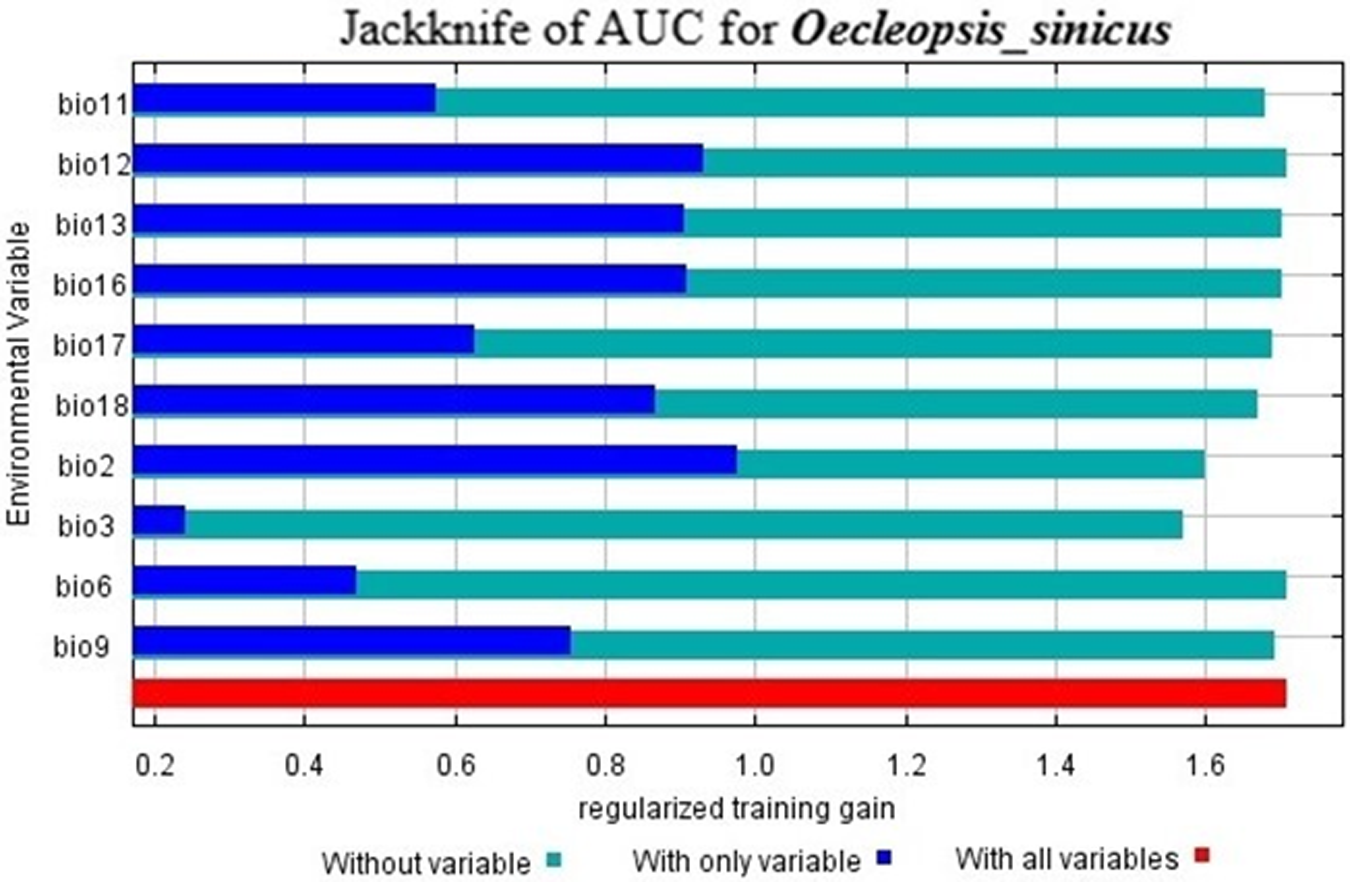
The potential global distribution of O. sinicus was projected using MaxEnt 3.4.4 (http://biodiversityinformatics.amnh.org/open-source/maxent/, accessed 12 May 2025) under both current and future climate scenarios. To enhance model performance and reduce overfitting, we assessed four combinations of feature classes (FCs) (auto features, LQ, LQH, and LQHPT) alongside regularisation multipliers (RMs) that varied from 0.5 to 4.0 in increments of 0.5. A sampling bias file was generated using kernel density estimation of occurrence points in ArcGIS to account for spatial sampling bias and constrain the selection of background points. The best-fitting models were based on LQHPT FCs, with a maximum of 5,000 iterations, 10,000 background points, and a logistic output format, using a fixed random seed for reproducibility. A 10-fold cross-validation method was used to test the model. The data were randomly split into 10 segments, and 9 were used for training, with 1 as a validation set. This method ensured that every occurrence record was included in both the training and validation phases. Additionally, to test model robustness and predictive performance, we partitioned the data such that 75% was randomly allocated to a training set, with 25% held out for independent testing. The environmental factors influencing the distribution of O. sinicus were identified through the results of the jackknife test and response curves (fig. 4). The best model was chosen by evaluating the area under the curve (AUC) metrics for various combinations of FCs and RMs. It was demonstrated that the AUC significantly correlates with the model’s predicted outcome efficiency; hence, the MaxEnt model was evaluated using a threshold-independent ROC curve and AUC with performance categories defined as: unsatisfactory (AUC < 0.6), poor (0.6–0.7), fair (0.7–0.8), good (0.8–0.9), and excellent (>0.9). Suitable and unsuitable habitats were defined using ETSAS, which represents equal training sensitivity and specificity.
The significance of environmental variables is evaluated using the jackknife test.

Figure 4 Long description
The bar graph title reads Jackknife of AUC for Oecleopsis underscore sinicus. The horizontal axis label reads Regularized training gain. Tick labels shown are 0.2, 0.4, 0.6, 0.8, 1.0, 1.2, 1.4, 1.6. The vertical axis label reads Error variables. Category labels shown are bio11, bio12, bio13, bio15, bio17, bio18, bio2, bio3, bio6, bio9. Legend labels shown are Without variable, With only variable, With all variables. For each error variable, three horizontal bars are shown corresponding to the legend labels. bio11: Without variable about 0.6; With only variable about 1.7; With all variables about 1.7. bio12: Without variable about 1.0; With only variable about 1.7; With all variables about 1.7. bio13: Without variable about 1.0; With only variable about 1.7; With all variables about 1.7. bio15: Without variable about 1.0; With only variable about 1.7; With all variables about 1.7. bio17: Without variable about 0.6; With only variable about 1.7; With all variables about 1.7. bio18: Without variable about 0.8; With only variable about 1.7; With all variables about 1.7. bio2: Without variable about 1.0; With only variable about 1.6; With all variables about 1.6. bio3: Without variable about 0.3; With only variable about 1.5; With all variables about 1.5. bio6: Without variable about 0.5; With only variable about 1.7; With all variables about 1.7. bio9: Without variable about 0.8; With only variable about 1.7; With all variables about 1.7.
Classification of suitable habitats
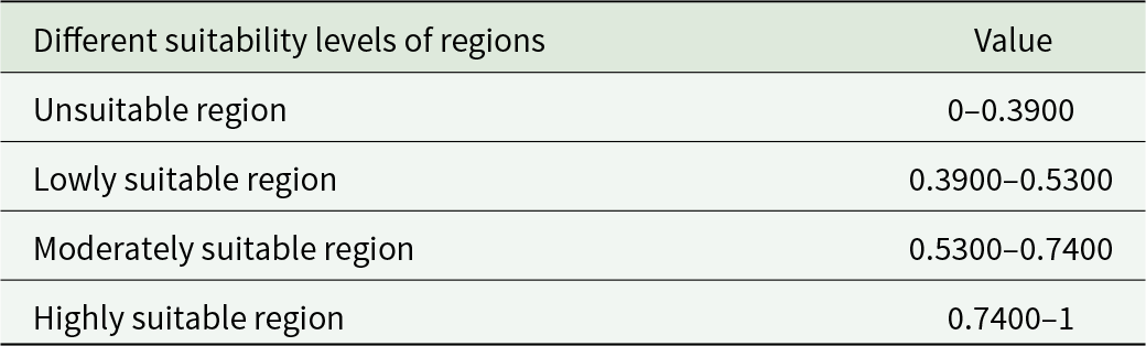
SDM Toolbox 10.9 and ArcGIS 10.8.2 are used to analyse changes in the distribution of O. sinicus under several climate scenarios. The distribution results for O. sinicus are categorised into four groups based on the output of the ETAS threshold: unsuitable environment (0–39), poorly suited habitat (0.39–0.53), moderately suitable habitat (0.53–0.74), and very suitable habitat (0.74–1) (table 1). To determine the distribution changes based on future climatic scenarios, the current and future results are compared using SDM Toolbox 10.9 and classified into four categories: no occupancy, no change, range contraction, and range expansion.
The Environmental Threat Assessment System threshold results demonstrated four levels of their suitability for O. sinicus geographic areas

Table 1 Long description
The table defines four suitability categories for O. sinicus based on a numeric index ranging from 0 to 1. Areas are classified as unsuitable from 0 to 0.3900. Low suitability spans 0.3900 to 0.5300, and moderate suitability spans 0.5300 to 0.7400. High suitability covers 0.7400 up to 1. The categories progress in order of increasing suitability as the index value increases. Values that fall exactly on a boundary may depend on the study’s classification rule for whether endpoints are included.
Distribution change estimation
To evaluate how O. sinicus might spread in response to climate change, several methods were utilised. The zonal statistics tool was implemented in ArcGIS 10.8.2 to define the potential habitat of these species under different climatic conditions and to identify the appropriate habitat type. Currently, appropriate areas were compared with those that would be appropriate in the future, considering the presence or absence of currently occupied areas. This analysis employed binary models and distribution maps to classify habitats as suitable or unsuitable. The distribution changes in the current and the project’s future scenarios were assessed using binary SDM tools in the SDM toolbox.
Results
MaxEnt model performance and key environmental variables
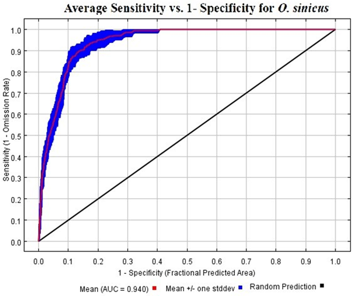
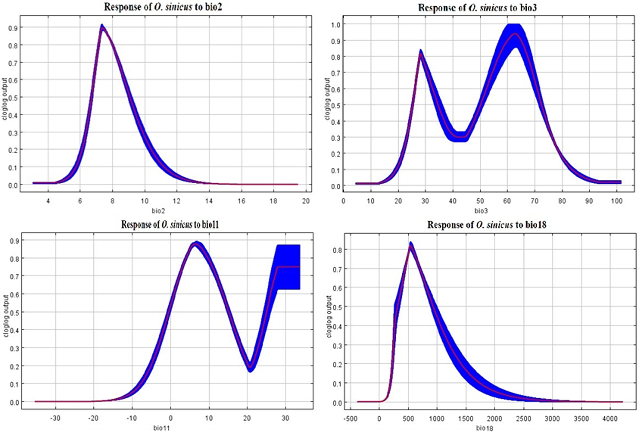
To prevent overfitting, we screened the distribution sites of O. sinicus and evaluated different combinations of FCs across various RM values. AUC scores peaked at RM = 1.5 across all models, with LQHPT yielding the highest accuracy. The optimal configuration for O. sinicus was LQHPT at RM = 1.5, with an AUC value of 0.940 (fig. 5). The AUC value of 0.940 for O. sinicus demonstrates that LQHPT are the most effective FC for modelling O. sinicus distributions and indicates excellent model performance in predicting suitable habitat areas for this species. Five environmental variables had the greatest impact on the potential suitable area for O. sinicus (table S1, fig. 6): Precipitation of the warmest quarter (Bio 18), Mean diurnal range (BIO2), Isothermality (Bio3), Annual precipitation (BIO12), and Mean temperature of the coldest quarter (BIO11), with percent contributions of 33.3%, 24%, 17%, 14.6%, and 4.6%, respectively. These five variables cumulatively contributed 93.8% to the model.
Area under the curves for O. sinicus distribution models in the current environmental conditions.

Figure 5 Long description
Average Sensitivity vs. 1- Specificity for O. sinicus The graph shows a receiver operating characteristic plot. The horizontal axis is labeled 1 minus Specificity (Fractional Predicted Area), ranging from 0.0 to 1.0 with tick marks at 0.1 intervals. The vertical axis is labeled Sensitivity (1 minus Omission Rate), ranging from 0.0 to 1.0 with tick marks at 0.1 intervals. A thick blue curve starts near (0.0, 0.0), rises steeply and then approaches the top boundary. The curve passes near (0.05, 0.70), (0.10, 0.85), (0.20, 0.95) and reaches about (0.40, 1.00), then continues along the top edge near sensitivity 1.0. A red line closely follows the blue curve and is shown with small vertical red error bars at multiple points along the curve. A black diagonal line runs from (0.0, 0.0) to (1.0, 1.0). The legend lists: Mean AUC equals 0.940, Mean plus or minus one standard deviation and Random Prediction.
Contribution of variables to habitat suitability of O. sinicus in Asia.

Figure 6 Long description
The image A showing the title “Response of O. sinicus to bio2”. The horizontal axis label is “bio2” with values from 4 to 20. The vertical axis label is “Cloglog output” with values from 0.0 to 0.9. A single curve rises from near 0.0 at bio2 about 4, reaches about 0.9 near bio2 about 8, then declines to near 0.0 by bio2 about 14 and stays near 0.0 through bio2 20. The image B showing the title “Response of O. sinicus to bio3”. The horizontal axis label is “bio3” with values from 0 to 100. The vertical axis label is “Cloglog output” with values from 0.0 to 1.0. A curve rises from near 0.0 at bio3 about 10, reaches about 0.8 near bio3 about 30, drops to about 0.3 near bio3 about 45, rises again to about 1.0 near bio3 about 70, then declines to near 0.0 by bio3 about 95. The image C showing the title “Response of O. sinicus to bio11”. The horizontal axis label is “bio11” with values from negative 30 to 30. The vertical axis label is “Cloglog output” with values from 0.0 to 0.9. A curve stays near 0.0 from bio11 negative 30 to about negative 10, rises to about 0.9 near bio11 about 10, declines to about 0.2 near bio11 about 22, then rises to about 0.8 to 0.9 near bio11 about 30. The image D showing the title “Response of O. sinicus to bio18”. The horizontal axis label is “bio18” with values from negative 500 to 4000. The vertical axis label is “Cloglog output” with values from 0.0 to 0.9. A curve rises from near 0.0 at bio18 about 0, reaches about 0.9 near bio18 about 500, then declines gradually to near 0.0 by bio18 about 2500 and stays near 0.0 through bio18 4000.
Suitable habitat and potential distribution of O. sinicus under current climate scenarios
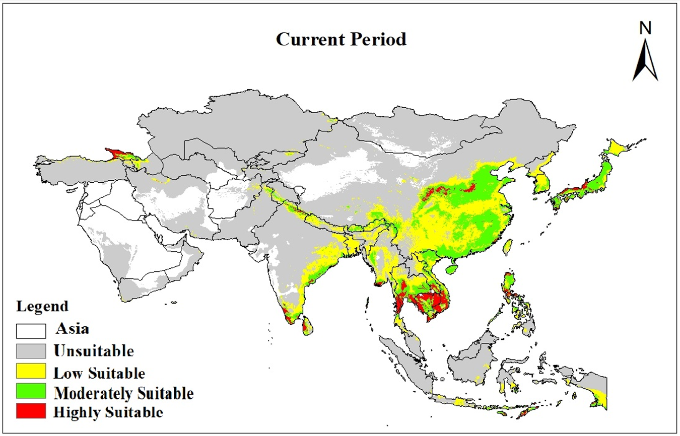
According to the ETSAS threshold, O. sinicus is expected to have adequate habitat to sustain this endemic species under current climatic conditions in Asia. The majority of suitable habitat is situated in southeastern Asia, with a smaller portion located in western Asia. Nevertheless, the medium- and high-favourable environment for O. sinicus is predominantly expanded from southeastern to northwestern Asia (fig. 7). Under current climate scenarios, suitable habitats for O. sinicus are projected to cover 114.77672 × 10⁴ km2 in Asia (25% of the study area). Highly suitable habitats cover 95.8902 × 10⁴ km2 (2.15% of area). Combined moderately and highly suitable habitats encompass 511.0572 × 10⁴ km2 (11.46% of area), distributed across southeastern and northwestern Asian plains (fig. 7).
Potentially suitable distribution areas for O. sinicus under current climatic projections.

Figure 7 Long description
The map of Asia illustrates habitat suitability for O. sinicus under current climatic conditions. The legend categorizes areas as unsuitable, low suitable, moderately suitable and highly suitable. Unsuitable areas are widespread across central and northern Asia. Low suitable regions are primarily in eastern Asia, including parts of China and Japan. Moderately suitable habitats are concentrated in southeastern Asia, extending into parts of China and India. Highly suitable areas are found in southeastern Asia, particularly in regions of Vietnam and Thailand. The map uses directional indicators, with north marked at the top, to show spatial distribution patterns.
Predicting O. sinicus distribution under future climate scenarios
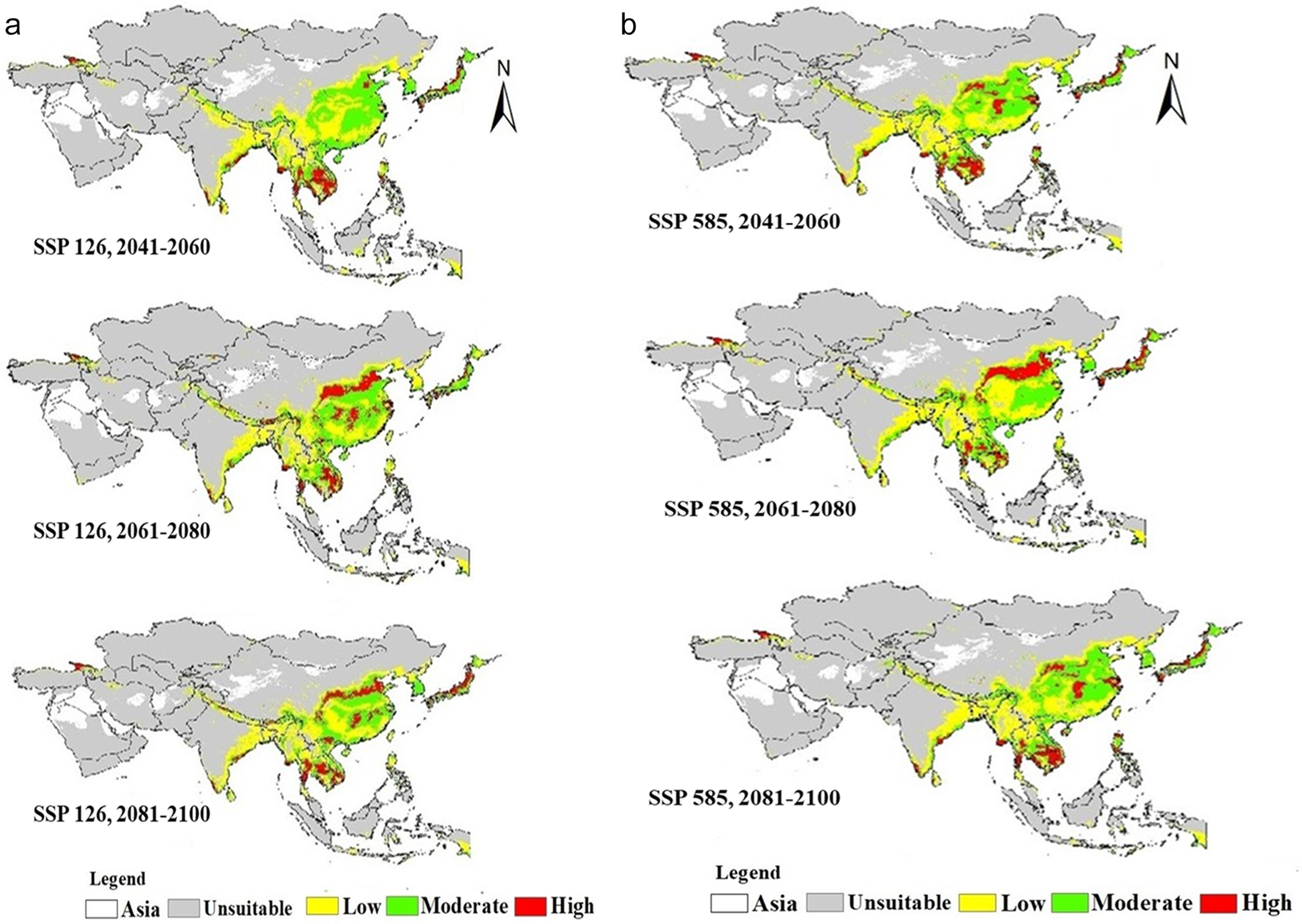
Suitable habitats for O. sinicus show significant variation across different SSPs under future climate scenarios (fig. 8a and table S4). Under all climate scenarios (2041–2060, 2061–2080, and 2081–2100 under SSP126 and SSP585) (fig. 8a and table S3), the suitable habitat for O. sinicus is projected to increase continuously. Under the 2041–2060 climate scenario, the potentially suitable habitats of O. sinicus in Asia are projected to increase to 128.80129 × 10⁴ km2 (SSP126) and 127.90871 × 10⁴ km2 (SSP585) (fig. 8a and table S3). These potentially suitable habitats are estimated to occupy 28.9% (SSP126) and 28.70% (SSP585) of the study area, respectively (table S3). Under the 2061–2080 climate scenario, the estimated potentially suitable habitats for O. sinicus are 122.04426 × 10⁴ km2 (SSP126) and 1,283.9887 × 10⁴ km2 (SSP585) (fig. 8a and table S3). The projected suitable habitats for O. sinicus correspond to an estimated 27.38% (SSP126) and 28.80% (SSP585) of the study area (table S3). Under the 2081–2100 climate scenario, the potential suitable habitats of O. sinicus are estimated to be 124.51091 × 10⁴ km2 (SSP126) and 124.58805 × 10⁴ km2 (SSP585) (fig. 8a, b and table S3).
(a) Suitability areas by O. sinicus in the future (SSP 126). (b) Suitability areas by O. sinicus in the future (SSP 585).

Figure 8 Long description
A) Maps depict habitat suitability for O. sinicus in Asia under SSP 126 for 2041–2060, 2061–2080 and 2081–2100. High suitability areas are concentrated in China, the Korean Peninsula and Japan, with moderate suitability extending to Indochina and India. B) Maps show suitability under SSP 585 for the same periods, with similar high suitability regions. The legend indicates suitability levels: Unsuitable (gray), Low (yellow), Moderate (green), High (red). Asia is the basemap and unsuitable areas are gray. North is indicated at the top by an arrow. The maps illustrate spatial shifts and expansions in suitable habitats over time.
Suitable habitat changes under future climate projections
The results of our analysis show that the highly suitable habitats of O. sinicus under future climate scenarios are mainly distributed in Sichuan, Guangxi, and small areas in Guangdong, Guizhou, and Fujian provinces. The moderately suitable ecological conditions are found in Hubei, Shaanxi, Gansu, Sichuan, Zhejiang, Fujian, Jiangxi, Hunan, Guizhou, Guangxi, Guangdong, as well as small portions of Xizang and Anhui provinces. The suitable habitat area expands from southeastern to northwestern Asia. The appropriate habitat for O. sinicus increases under projected climate scenarios compared to current conditions. During 2041–2060, the potential distribution is projected to increase by 518.9169 × 10⁴ km2 under SSP126 and 981.2836 × 10⁴ km2 under SSP585, expanding by 45.2% and 85.1%, respectively. For 2061–2080, the potential distribution in Asia is projected to increase to 482.8101 × 10⁴ km2 (SSP126) and 514.1945 × 10⁴ km2 (SSP585), with Southeast Asia showing increases of 42.6% and 44.7%. Under the 2081–2100 scenarios, the potential distribution is estimated to increase by 511.7527 × 10⁴ km2 (SSP126) and 570.9165 × 10⁴ km2 (SSP585), representing 44.59% and 49.7% increases in the total study area compared to the current distribution (table S4).
Discussion
Model validation and future projections
SDMs produce accurate results only when both the input data (species occurrence records) and software parameters are of high quality (Zhang et al., Reference Zhang, Wang, Wei, Sun, Zhou and Zhang2024; Zhao et al., Reference Zhao, Li and Chen2024; DEFRA (Department for Environment, Food & Rural Affairs), 2025). MaxEnt modelling revealed that O. sinicus exhibits a strong predictive performance, with AUC values consistently exceeding 0.94. This indicates that this model can reliably forecast both the current and prospective ranges of this indigenous planthopper taxon. Temperature-related variables were shown to influence the distribution of similar pest species in the United States using the MaxEnt model (Wakie et al., Reference Wakie, Neven, Yee and Lu2020). Recognising the importance of temperature helps researchers feel appreciated for their focus on critical environmental factors. Consistent with studies on distribution modelling of other insects (Wei et al., Reference Wei, Zhao, Zhao and Zhang2018; Abou-Shaara et al., Reference Abou-Shaara, Alashaal, Hosni, Nasser, Ansari and Alharbi2021; Amaro et al., Reference Amaro, Fidelis, de Medeiros and da Silva2022), temperature-related variables were more important than precipitation-related variables in our model. It indicates that insects are poikilotherms, that their physiological processes are influenced by temperature (Zhang et al., Reference Zhang, Zhao, Wang and Liu2023), and that their geographical distribution is predetermined. Projections of both SSP126 and SSP585 scenarios indicate that the appropriate habitat of O. sinicus is likely to increase significantly during all future years between 2041 and 2100.
Distribution of O. sinicus under climate change
Climate change projections indicate that the extent of appropriate habitat will rise significantly in both scenarios (SSP126 & SSP585), by 42.6–85.1%, according to the time frame and the emission scenarios (Ali et al., Reference Ali, Hou and Tahir2023; Dunne et al., Reference Dunne, Williams and Martinez2002; Brooks et al., Reference Brooks, Mittermeier, da Fonseca, Gerlach, Hoffmann, Lamoreux, Mittermeier, Pilgrim and Rodrigues2006; Tylianakis et al., Reference Tylianakis, Laliberte, Nielsen and Bascompte2010). Thus, habitat expansion is likely to be observed in southeastern and northwestern Asia, indicating that rising temperatures can enhance habitat suitability across larger landscapes and alleviate thermal constraints in northwestern regions previously regarded as unfavourable (Tylianakis et al., Reference Tylianakis, Laliberte, Nielsen and Bascompte2010). The reduction in temperature extremes and the alteration of precipitation patterns are contributing to the anticipated eastward movement. This alteration can affect agricultural areas, where pest problems can become more complex, or intensify the risk of O. sinicus penetration into agricultural regions (Raina et al., Reference Raina, Chauhan, Tayal, Pandey, Srivastava and Kindlmann2021). In addition, insect distribution will be heavily influenced by altitudinal variables, according to previous research (Schuldt and Assmann, Reference Schuldt and Assmann2009, Reference Schuldt and Assmann2011). Nevertheless, the influence of altitude could not be as significant in this research as that of the temperature and precipitation variables. Climate matching implies that a rising climate has promoted species expansion into the northwestern regions, with climate challenges surpassing past thermal limitations and sufficient moisture regimes owing to shifting precipitation patterns. The habitat expansion potential means that regions previously restricted by low winter temperatures can gradually become climatically favourable, leading to the successful establishment of the population in the areas that were historically marginal or inaccessible to the species (Burlakova et al., Reference Burlakova, Karatayev, Karatayev, May, Bennett and Cook2011; Seebens et al., Reference Seebens, Blackburn, Dyer, Genovesi, Hulme, Jeschke, Pagad, Pysek, Winter, Arianoutsou, Bacher, Blasius, Brundu, Capinha, Celesti-Grapow, Dawson, Dullinger, Fuentes, Jager, Kartesz, Kenis, Kreft, Kuhn, Lenzner, Liebhold, Mosena, Moser, Nishino, Pearman, Pergl, Rabitsch, Rojas-Sandoval, Roques, Rorke, Rossinelli, Roy, Scalera, Schindler, Štajerová, Tokarska-Guzik, van Kleunen, Walker, Weigelt, Yamanaka and Essl2017).
Implications for pest management and ecological dynamics
O. sinicus currently displays an extended southeastern Asian distribution pattern, which is expected to expand substantially under future climate change, potentially leading to extensive colonisation of previously inaccessible regions across wider Asian habitats (Wang and Hijmans, Reference Wang, Hijmans and Nriagu2019). This species is highly sensitive to precipitation patterns, especially in summer, and moderately sensitive to temperature changes, which means that climate change will affect Southeast Asia in regionally complex ways, shifting habitat suitability northwestward while enhancing conditions in existing southeastern strongholds (Urban, Reference Urban2017; Sun et al., Reference Sun, Wang, Zhou, Wang, Wang, Lyu and Li2020).
It has been projected that, with the expansion of suitable habitat, pest pressure on agricultural systems will also increase across Southeast Asia, and, in some cases, management will become more difficult as O. sinicus colonises previously marginal areas. Although climate change may have beneficial effects on the species, such as increased habitat availability (42.6–85.1%), rapid changes in range distributions can cause ecological disturbances and novel pest-crop interactions, which should be addressed through adaptive management strategies (Ali and Zhou, Reference Ali and Zhuo2025; Seebens et al., Reference Seebens, Blackburn, Dyer, Genovesi, Hulme, Jeschke, Pagad, Pysek, Winter, Arianoutsou, Bacher, Blasius, Brundu, Capinha, Celesti-Grapow, Dawson, Dullinger, Fuentes, Jager, Kartesz, Kenis, Kreft, Kuhn, Lenzner, Liebhold, Mosena, Moser, Nishino, Pearman, Pergl, Rabitsch, Rojas-Sandoval, Roques, Rorke, Rossinelli, Roy, Scalera, Schindler, Štajerová, Tokarska-Guzik, van Kleunen, Walker, Weigelt, Yamanaka and Essl2017). The increase in these pressures is due to anthropogenic factors that destroy habitats through urban development, deforestation, pesticide use, and overgrazing, that can increase the effect of climatic changes on the ecological system and the survival of species (Sun et al., Reference Sun, Wang, Zhou, Wang, Wang, Lyu and Li2020). Hence, to efficiently address the expanding distribution of O. sinicus, the MaxEnt model’s findings suggest that affected areas should implement comprehensive monitoring schemes and adaptive pest control strategies that account for range shifts resulting from climate change.
Research gaps and future directions in SDM
Other key influences on species distribution are not studied in this work, including the response of host plants to climate change, natural enemies and competition, patterns of human activity and microclimate variability, extreme weather events, adaptive evolution, and phenotypic plasticity. To enhance the accuracy of predictions and management strategies, future studies should combine field monitoring, interaction studies, and high-resolution datasets.
Conclusion
MaxEnt modelling projects that suitable habitat for O. sinicus will expand by 44.6–49.7% (511.8–570.9 × 10⁴ km2) by 2100 under the SSP2-4.5 and SSP5-8.5 scenarios. The species is expected to shift its distribution northwestward across Asia. Notably, East Asia is projected to experience the most significant expansion, particularly in northwestern China, including the provinces of Gansu and Shaanxi. Under climate change scenarios based on MaxEnt modelling, the species is expected to move. The key bioclimatic variable influencing the potential distribution of this East Asian agricultural pest was precipitation of the warmest quarter (Bio18, 33.3% contribution). This study is the first quantitative assessment of the entire species distribution of O. sinicus across the Asian continent under future climate conditions and is expected to serve as the basis for proactive pest management planning. Consequently, based on these projections, we suggest that surveillance and monitoring programs should be established in the high-risk expansion areas that are likely to emerge in Asia in the near future to detect the range shifts early. Limitations of this study include reliance on a single GCM, exclusion of biotic interactions, and unmodelled dispersal constraints. Future research using multi-model ensemble approaches and integrating these factors will refine regional-level management strategies.
Supplementary material
The supplementary material for this article can be found at https://doi.org/10.1017/S0007485326100868.
Acknowledgements
The authors express their sincere gratitude to Prof. John Richard Schrock (Emporia State University, Emporia, USA) for reviewing the manuscript and suggesting valuable improvements and to William L. Murphy, Research Collaborator, U.S. National Museum of Natural History, Washington, DC, USA, for his extensive assistance with editorial, formatting, and English-language proofreading of several versions of the manuscript. This research was financially supported by the National Natural Science Foundation of China (Nos. 32170475, 31750002).
Author contributions
Muhammad Aqib Idrees: Writing – original draft, software, methodology, formal analysis. Qin Daozheng: supervision, conceptualisation, resources, writing – review & editing, funding acquisition, data curation.
Financial support
This work was supported by the National Natural Science Foundation of China (grant numbers 32170475, 31672340, 31750002).
Competing interests
The author(s) declare no competing interests.
Availability of data and materials
Data will be made available on request.
Ethical approval
Not applicable