1 Introduction
Internal solitary waves (ISWs) continue to attract burgeoning interest, not least because of their pervasiveness in many marine and freshwater environments (Horn, Imberger & Ivey Reference Horn, Imberger and Ivey2001; Nash & Moum Reference Nash and Moum2005; Helfrich & Melville Reference Helfrich and Melville2006; Groeskamp, Nauw & Maas Reference Groeskamp, Nauw and Maas2011; Lamb Reference Lamb2014; Bourgault, Galbraith & Chavanne Reference Bourgault, Galbraith and Chavanne2016; Boegman & Stastna Reference Boegman and Stastna2019). They propagate on density interfaces in stably stratified fluid systems and may be characterised generally as nonlinear, dispersive waves of quasi-permanent form with an amplitude comparable with the thickness of the interface on which they travel and also, in many cases of interest, the overall depth of the fluid system in question (see e.g. Grue et al. Reference Grue, Jensen, Rusås and Sveen1999; Grimshaw Reference Grimshaw2014).
In linear theory, sets of modal solutions exist for large amplitude ISWs propagating in bounded, stratified fluids but, for most cases of geophysical interest, over
 $90\,\%$
of kinetic energy of the nonlinear baroclinic modes is contained within the first two modes (MacKinnon & Gregg Reference MacKinnon and Gregg2003). ISWs of mode-1 displace isopycnals in one direction only and can be either waves of elevation or depression, depending on whether the displacement is, respectively, parallel or anti-parallel to the gravitational acceleration vector. Mode-2 waves, on the other hand, displace isopycnals in opposing directions (Yang et al.
Reference Yang, Fang, Tang and Ramp2010). They may be convex in form, in which case upper and lower isopycnals are displaced upward and downward respectively with respect to the mid plane of the pycnocline, or concave (concave mode-2 waves require a relatively thick pycnocline on which to propagate and are seldom observed naturally in marine and freshwater environments) in which case the opposite is true (upper and lower isopycnals are displaced downward and upward, respectively, with respect to the mid plane of the pycnocline).
Mode-1 waves are referred to as ISWs as they travel faster than all other mode numbers and nonlinear mode-1 waves outpace linear waves. Hence, they propagate away from any initial disturbance and achieve a solitary state. Mode-2 waves, even in the long wave limit, cannot have wave speeds that are faster than a finite-length mode-1 wave. Thus, whenever mode-2 waves are observed, they are accompanied by a tail of mode-1 waves. In terms of linear wave theory, the phase speed of the mode-1 tail matches the propagation speed of the mode-2 leading wave. However, the mode-1 group velocity is smaller than the phase velocity and thus energy is slowly drained from the mode-2 wave. For this reason mode-2 waves are often referred to as solitary-like as they will slowly decay. This scenario has been formally justified using asymptotics beyond all orders in Akylas & Grimshaw (Reference Akylas and Grimshaw1992).
In recent years, most attention has been concentrated on mode-1 ISWs because of their scale and importance in the oceans (Osborne & Burch Reference Osborne and Burch1980; Duda et al. Reference Duda, Lynch, Beardsley, Ramp, Chiu, Tang and Yang2004; Van Gastel et al. Reference Van Gastel, Ivey, Meuleners, Antenucci and Fringer2009) and their potential threat to the integrity of offshore structures (see, for example, Hyder et al. Reference Hyder, Jeans, Cauquil and Nerzic2005). Nevertheless, many field observations have illustrated that mode-2 waves also occur widely in aquatic environments and, furthermore, they have the potential to play an important role in interior and boundary mixing processes (Duda et al. Reference Duda, Lynch, Beardsley, Ramp, Chiu, Tang and Yang2004; Boegman, Ivey & Imberger Reference Boegman, Ivey and Imberger2005; Yang et al. Reference Yang, Fang, Chang, Ramp, Kao and Tang2009; Shroyer, Moum & Nash Reference Shroyer, Moum and Nash2010; Yang et al. Reference Yang, Fang, Tang and Ramp2010; Guo & Chen Reference Guo and Chen2012; Liu et al. Reference Liu, Su, Hsu, Kuo and Ho2013). The recent high resolution synthetic aperture radar observations of Magalhaes & da Silva (Reference Magalhaes and da Silva2018) suggest that mode-2 ISWs may have been overlooked in previous remote sensing images and are more widespread than thought previously.
There is already a substantial literature on the modelling of mode-2 waves for cases of constant depth and many of these studies (Davis & Acrivos Reference Davis and Acrivos1967; Kao & Pao Reference Kao and Pao1980; Maxworthy Reference Maxworthy1980; Stamp & Jacka Reference Stamp and Jacka1995; Schmidt Reference Schmidt1998; Terez & Knio Reference Terez and Knio1998; Stastna & Peltier Reference Stastna and Peltier2005; Gavrilov & Lyapidevski Reference Gavrilov and Lyapidevski2009; Salloum, Knio & Brandt Reference Salloum, Knio and Brandt2012; Olsthoorn, Baglaenko & Stastna Reference Olsthoorn, Baglaenko and Stastna2013; Brandt & Shipley Reference Brandt and Shipley2014; Carr, Davies & Hoebers Reference Carr, Davies and Hoebers2015; Deepwell & Stastna Reference Deepwell and Stastna2016; Cheng et al. Reference Cheng, Hsieh, Hwang and Hsu2018) have contributed significantly to our understanding of the generation mechanisms of mode-2 waves, their structural, stability and kinematic properties and their ability to transport mass. Much recent interest has focussed on the effects of bottom topography upon the above properties, with laboratory and computational studies being undertaken by Gavrilov & Lyapidevski (Reference Gavrilov and Lyapidevski2011), Guo & Chen (Reference Guo and Chen2012), Cheng et al. (Reference Cheng, Hsieh, Hsu and Hwang2017) and Yuan, Grimshaw & Johnson (Reference Yuan, Grimshaw and Johnson2018) for slope-shelf topography and Deepwell et al. (Reference Deepwell, Stastna, Carr and Davies2017) for the case of a train of mode-2 ISWs encountering a narrow, two-dimensional, Gaussian-profile ridge. The combined numerical and laboratory investigation undertaken in the Deepwell et al. (Reference Deepwell, Stastna, Carr and Davies2017) study provided, for the first time, clear indications of flow separation and vortex formation on the upward boundary slope of the topography as a characteristic property of shoaling mode-2 waves of large and moderate amplitude. The numerical modelling study by Cheng et al. (Reference Cheng, Hsieh, Hsu and Hwang2017) considered the distortion caused to mode-2 waves by passage over a combined slope-shelf topography placed in a channel having the same dimensions and gate release wave generation mechanism in the experiments described by Carr et al. (Reference Carr, Davies and Hoebers2015), Deepwell et al. (Reference Deepwell, Stastna, Carr and Davies2017) and the present investigation. Test runs conducted by Cheng et al. (Reference Cheng, Hsieh, Hsu and Hwang2017) to replicate the laboratory study by Carr et al. (Reference Carr, Davies and Hoebers2015) for constant depth conditions showed excellent agreement between numerical simulations and laboratory data. This finding adds particular relevance to comparisons of the shoaling behaviours observed by Cheng et al. (Reference Cheng, Hsieh, Hsu and Hwang2017) for the slope-shelf topography with those reported herein for constant slope cases (without a shelf).
Cheng et al. (Reference Cheng, Hsieh, Hsu and Hwang2017) considered the same undisturbed, stable density configuration as the present paper, namely two homogeneous layers of different density but equal thickness, separated by a thin pycnocline. The mid-level of the undisturbed pycnocline was prescribed to be always above the plateau section of the slope-shelf topography and a single slope with a fixed length and angle
 $\unicode[STIX]{x1D703}$
 $(\unicode[STIX]{x1D703}=6^{\circ };s=\tan \unicode[STIX]{x1D703}=0.105)$
was considered. With such an arrangement, the distortion of an incident mode-2 wave train by the topography is due partly to shoaling on the slope section and partly to adjustment to the constant depth (but unequal fluid layer thicknesses) on the plateau. For the cases investigated by Cheng et al. (Reference Cheng, Hsieh, Hsu and Hwang2017), the flow development during the shoaling phase indicated significant distortion of the lower bounding isopycnals of the leading wave, a significant induced down slope flow between the wave and the slope boundary and, for sufficiently high amplitudes, the generation of boundary vortices by flow separation. In this paper, the degree of the slope is varied, there is no shelf and attention is focussed on the wave/slope interaction including investigation of the fluid dynamics when the pycnocline intersects the slope.
Many of the above flow features are also observed with shoaling mode-1 waves, where several extensive laboratory and numerical model studies have been undertaken (see, for example, Boegman et al. (Reference Boegman, Ivey and Imberger2005), Aghsaee, Boegman & Lamb (Reference Aghsaee, Boegman and Lamb2010), Sutherland, Barrett & Ivey (Reference Sutherland, Barrett and Ivey2013) and Nakayama et al. (Reference Nakayama, Sato, Shimizu and Boegman2019) and references therein). These studies have been successful in not only delineating the different processes determining the shoaling behaviour of mode-1 ISWs for different combinations of boundary slope
 $s$
and wave slope
 $s_{w}(=a/L_{w})$
but also characterising and classifying the shoaling regimes in terms of these parameters. For a given wave amplitude
 $a$
and wavelength
 $L_{w}$
, transformation of the mode-1 form into higher harmonics (fission) is observed for relatively shallow slope angles, as the wave passes through the turning point location where the polarity changes (Lamb Reference Lamb2014). Reflection (with no breaking) is seen for very steep slopes. For intermediate (moderate to steep) slopes, several different types (surging, collapsing, collapsing plunging, plunging) of wave breaking occur, with the breaking regimes being classified conveniently in terms of
 $s,s_{w}$
and the relative values of the time scales characterising the individual wave breaking processes (Aghsaee et al.
Reference Aghsaee, Boegman and Lamb2010; Nakayama et al.
Reference Nakayama, Sato, Shimizu and Boegman2019). Sutherland et al. (Reference Sutherland, Barrett and Ivey2013) demonstrate that shoaling-induced breaking regimes of mode-1 ISWs can be classified successfully in terms of the bed slope
 $s$
and an internal Iribarren (
 $Ir$
is a modified version of the equivalent shoaling parameter (e.g. Hughes Reference Hughes2004b
) for surface waves breaking on a beach) number
 $Ir=s/(s_{w})^{1/2}$
, subject to careful definition of the length scale
 $L_{w}$
. A thorough review of these studies and related field observations can be found in Boegman & Stastna (Reference Boegman and Stastna2019). In this paper, a similar range of
 $s$
and
 $Ir$
to those in the studies above are considered. It is found, however, that mode-2 ISWs do not exhibit the same range of breaking (surging, collapsing, plunging) as mode-1 waves do during the shoaling process. The extent to which the above studies of mode-1 shoaling waves of depression are able to inform interpretation of counterpart observations of mode-2 shoaling under similar conditions is a key consideration in the present study. Whilst breaking characteristics are found to be different, similarities are seen in the bottom boundary layer flow.
Here, a combined investigation comprising laboratory experiments and numerical simulations has been undertaken to investigate parametrically the propagation of a train of mode-2 ISWs waves over a uniformly sloping, solid boundary. The objectives of the study have been to delineate the detailed shoaling behaviour of the waves over a wide range of external conditions, to map the velocity and vorticity fields induced by the shoaling waves and to compare the numerical modelling predictions with the data from the laboratory experiments that they replicate. Furthermore, an important aim is to exploit the versatility of the numerical model flume to overcome the finite-length restriction of the laboratory counterpart flume for cases in which the slope is too shallow for the wave to undergo full shoaling development before reaching the end wall.
The paper is outlined as follows. In §§ 2 and 3, the experimental and numerical methods are respectively described. In § 4 results are presented illustrating the dynamics associated with shoaling mode-2 ISWs. Finally, in §§ 5 and 6 discussion and conclusions are given respectively.
2 Experimental set-up and procedure
2.1 Physical arrangement and wave generation
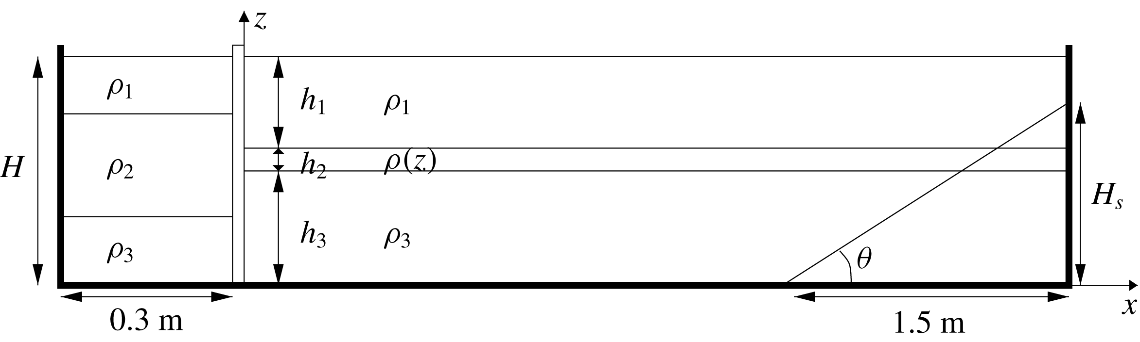
Schematic diagram of the laboratory arrangement (not to scale).

A wave flume
 $6.4~\text{m}$
long,
 $0.4~\text{m}$
wide,
 $0.6~\text{m}$
high and of rectangular cross-section was divided into two sections by a vertical gate situated a distance
 $0.3~\text{m}$
from one end of the flume (see figure 1). Within a Cartesian coordinate system
 $(x,y,z)$
, the
 $x$
and
 $z$
directions denote, respectively, the horizontal direction of wave propagation and the vertical direction anti-parallel to the gravitational acceleration vector
 $\boldsymbol{g}=(0,0,-g)$
. The origin is chosen such that
 $x=0$
coincides with the horizontal location of the gate and
 $z=0$
coincides with the lower solid boundary of the water column. The gate extended to the bottom of the flume and was used to separate the main flume (
 $x>0$
) from the wave generating region (
 $x<0$
). An inclined, rigid, acrylic plate of vertical height
 $H_{s}$
and base length
 $1.5~\text{m}$
, was fixed to the bed of the flume to form a sloping boundary at the end of the channel. The background stratification in the main part of the flume consisted of upper and lower layers of miscible homogeneous brine solution of prescribed densities
 $\unicode[STIX]{x1D70C}_{1}=1024\pm 2~\text{kg}~\text{m}^{-3}$
and
 $\unicode[STIX]{x1D70C}_{3}=1045\pm 2~\text{kg}~\text{m}^{-3}$
respectively, and undisturbed thicknesses
 $h_{1}=0.137\pm 0.005~\text{m}$
and
 $h_{3}=0.142\pm 0.005~\text{m}$
respectively. The densities and the layer depths were measured using a hydrometer and micro-conductivity sensors respectively (see § 2.2 and Carr et al. (Reference Carr, Davies and Hoebers2015)). A pycnocline of undisturbed thickness of
 $h_{2}=0.021\pm 0.006~\text{m}$
and density,
 $\unicode[STIX]{x1D70C}(z)$
, which varied as a linear function of
 $z$
separated the two homogeneous layers. The stratification was formed by slowly dripping the layer of less dense fluid (
 $\unicode[STIX]{x1D70C}_{1}$
) through an array of floating sponges on to the denser layer (
 $\unicode[STIX]{x1D70C}_{3}$
) of fluid.
To generate a mode-2 ISW, the region behind the gate (
 $x<0$
) was stratified (again using a floating sponge arrangement) such that the upper and lower layers had densities that matched those in the respective upper and lower layers of the main section of the flume, while the middle layer, consisted of a volume of mixed fluid, of average density
 $\unicode[STIX]{x1D70C}_{2}=(\unicode[STIX]{x1D70C}_{1}+\unicode[STIX]{x1D70C}_{3})/2$
. The centre of the mixed layer (of density
 $\unicode[STIX]{x1D70C}_{2}$
) was arranged so that it coincided with the centre of the pycnocline (also of density
 $\unicode[STIX]{x1D70C}_{2}$
) in the main section of the flume. To facilitate this, the form of the stratification was precisely measured using micro-conductivity sensors (see § 2.2). The aspect ratio of the volume of fluid of density
 $\unicode[STIX]{x1D70C}_{2}$
behind the gate controls the wave amplitude, wave number and wave form (see Kao, Pan & Renouard Reference Kao, Pan and Renouard1985; Brandt & Shipley Reference Brandt and Shipley2014). The total water depth was
 $H$
(see figure 1).
The density difference,
 $\unicode[STIX]{x0394}\unicode[STIX]{x1D70C}=\unicode[STIX]{x1D70C}_{3}-\unicode[STIX]{x1D70C}_{1}$
, between layers was kept as constant as possible during the study, as was the total fluid depth
 $H=0.3\pm 0.001~\text{m}$
. Care was taken to make the thickness of the pycnocline,
 $h_{2}=0.021\pm 0.006~\text{m}$
, and the location of the pycnocline centre (mid-depth)
 $h_{3}+h_{2}/2=0.15\pm 0.003~\text{m}$
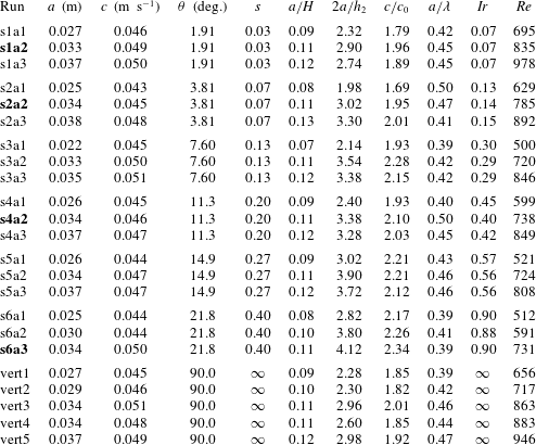
approximately constant throughout the study. However, the formation of the pycnocline was difficult to control precisely due to (i) disturbances to the pycnocline during filling and (ii) differences in filling times. Parametric changes were introduced by changing (i) the generating volume of mixed fluid behind the gate (in order to vary wave amplitude) and (ii) the slope steepness. Table 1 provides an overview of the 23 experiments that were performed. Bold entries highlight runs that are presented in detail in the paper; they are chosen to reflect laboratory observations at a constant non-dimensional wave amplitude of
 $a/H=0.11$
, over the range of slope steepness investigated.
Experimental parameters.
 $a$
is wave amplitude,
 $c$
is wave speed,
 $\unicode[STIX]{x1D703}$
is slope angle,
 $s=H_{s}/1.5$
is non-dimensional slope steepness,
 $c_{0}=\sqrt{gh_{2}\unicode[STIX]{x0394}\unicode[STIX]{x1D70C}/8\unicode[STIX]{x1D70C}_{2}}$
is the infinitesimal linear long mode-1 wave speed,
 $Ir=s/\sqrt{a/2\unicode[STIX]{x1D706}}$
is the Iribarren number, where
 $\unicode[STIX]{x1D706}$
is the wavelength measured at half-amplitude, and
 $Re=c_{0}a/\unicode[STIX]{x1D708}$
is the Reynolds number, where
 $\unicode[STIX]{x1D708}$
is the kinematic viscosity of water. Bold entries highlight runs that are presented in detail in the paper.

The experiment was initiated by the vertical removal of the gate which resulted in the generation of a rank-ordered train of mode-2 ISWs which propagated along the pycnocline into the main section of the flume. A Styrofoam lid was placed on top of the water column to minimise surface disturbances and aid comparison with numerical studies.
2.2 Flow measurement and flow visualisation
High precision, micro-conductivity sensors (Munro & Davies Reference Munro and Davies2009) were used to measure the form of the stratification. The sensors were mounted on on a rigid rack and pinion traverse system fitted with a potentiometer. The sensors were moved vertically through the water column and density profiles subsequently obtained by calibrating the potentiometer output and conductivity data against known values of height and fluid density respectively. An example of the stratification in the main section of the tank and behind the gate just prior to an experimental run can be seen in Carr et al. (Reference Carr, Davies and Hoebers2015) figure 3(a).
A vertical section in the mid-plane of the tank was illuminated by a continuous, collimated light sheet from an array of light boxes placed below the (transparent) base of the tank. Motions within this vertical light sheet were viewed and recorded from the side using three fixed digital video cameras set up outside the tank. The cameras (UNIQ UP-1830CL-12B) had a spatial resolution of
 $1372\times 1372$
pixels and they captured data at 30 f.p.s. The water column in the main section of the flume, was seeded with light-reflecting tracer particles having diameters in the range
 $150{-}300~\unicode[STIX]{x03BC}\text{m}$
. The particles had a buoyancy range such that they were neutrally buoyant throughout the depth of the water column. The three cameras were synchronised in time and positioned to have overlapping fields of view. The cameras were centred in the vertical direction on the pycnocline to avoid distortion and perspective errors in this portion of the flow field. The cameras were labelled from 1 to 3, with 1 and 3 being, respectively, the cameras closest to and furthest from the gate end of the flume.
The software package DigiFlow (Dalziel et al. Reference Dalziel, Carr, Sveen and Davies2007) was used to process the digital video records. The time series function of DigiFlow was used to measure wave speed, wave amplitude and wavelength. The particle image velocimetry (PIV) function in DigiFlow (Dalziel et al. Reference Dalziel, Carr, Sveen and Davies2007) was used to calculate continuous synoptic velocity and vorticity field data along the illuminated cross-section in the middle of the tank.
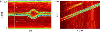
Figure 2(a) shows an example of a time series constructed by measuring the temporal changes in image pixel values in a prescribed column at a fixed horizontal coordinate in each frame of the experimental movie over a time interval
 $\unicode[STIX]{x0394}t$
. The time series is ordered sequentially from left to right. Such series were used to measure wave amplitude by tracing the maximum displacement of a streamline over the chosen time interval
 $\unicode[STIX]{x0394}t$
. Streamlines were traced at the top (
 $z=h_{3}+h_{2}$
) and bottom (
 $z=h_{3}$
) of the pycnocline and the average of the two measures taken to define wave amplitude,
 $a$
. This process was repeated at three fixed locations on any given camera viewing window over evenly spaced horizontal distances. The variance in measuring the amplitude was
 $4\,\%$
. In figure 2(b), an example of a time series constructed by measuring the temporal changes in image pixel values in a prescribed row of lateral extent
 $\unicode[STIX]{x0394}x$
at a fixed vertical coordinate in each frame of the experimental movie, over a time interval
 $\unicode[STIX]{x0394}t$
is presented. The time series is ordered sequentially from bottom to top. The vertical coordinate was chosen to be mid-way between the lower interface of the pycnocline and the maximum interface depth (
 $z=h_{3}-a/2$
), following Sutherland et al. (Reference Sutherland, Barrett and Ivey2013). The rightward advance of the wave can be seen in figure 2(b) as two bright bands, corresponding to the leading and trailing faces of the first mode-2 wave in the rank-ordered train. The wave speed,
 $c$
, was measured by fitting a straight line to the first bright band (leading face of the wave) and computing its gradient. It can be seen from figure 2(b) that the wave speed was constant (bright band is a straight line over the measurement period
 $\unicode[STIX]{x0394}t$
). The error in measuring
 $c$
in this way was less than
 $1\,\%$
. The half-wavelength,
 $\unicode[STIX]{x1D706}(=L_{w}/2)$
, was computed from the vertical time series (figure 2
a) by measuring the time it took the pycnocline to be displaced from
 $h_{3}$
to
 $h_{3}-a/2$
and multiplying the result by
 $2c$
. This process was repeated at three fixed locations on any given camera viewing window over evenly spaced horizontal distances. The variance in measuring the wavelength was
 $4\,\%$
. Error bars are omitted from all experimental data plots as the data marker size is bigger than the error bars in all cases.
(a) Vertical time series of light scattered from tracer particles, at
 $x=4.29~\text{m}$
with
 $\unicode[STIX]{x0394}t=22~\text{s}$
, (b) horizontal time series of light scattered from tracer particles, at
 $z=0.12~\text{m}$
, with
 $\unicode[STIX]{x0394}t=40.25~\text{s}$
and
 $\unicode[STIX]{x0394}x=1.16~\text{m}$
.

3 Numerical method
Numerical simulations were carried out with the pseudo-spectral code SPINS. The basic algorithmic design (e.g. the coordinate mapping method, numerical linear algebra methods, parallelisation strategy, etc.), as well as multiple validation exercises are described in Subich, Lamb & Stastna (Reference Subich, Lamb and Stastna2013). The code solves the stratified Navier Stokes equations under the Boussinesq approximation, and for this paper all simulations were carried out in two dimensions with no slip boundary conditions applied at the top and bottom boundaries. Since no slip boundary conditions on the end walls would lead to a ‘doubly clustered’ grid at the corners, free slip conditions on the left and right end walls were chosen to be employed there. This led to no change in the dynamics described below. Horizontal resolution was fixed at
 $1.5~\text{mm}$
for all simulations presented. This means that simulations with a double-length tank also doubled the number of points in the horizontal. The vertical resolution varied due to the presence of topography and the clustering of the Chebyshev points near the boundaries. Near the mid-depth the resolution was lowest, approximately 1.8 mm, while in the boundary layer it was less than 0.1 mm. Grid halving experiments were carried out to ensure all reported results were grid insensitive.
The code was initialised from a state of rest, with a density perturbation that mimicked the laboratory lock-release mechanism, save for a smoothing across the portion of the numerical domain that would be the lock barrier in the experiment. This smoothing is necessary due to the spectral nature of the code. In practice, such smoothing does not modify the ISWs generated, but does decrease the amount of turbulence near the release location. The code has been found to do an excellent job in reproducing experimental results, for example in propagation of mode-2 ISWs over isolated topography (Deepwell et al. Reference Deepwell, Stastna, Carr and Davies2017).
4 Results
4.1 Experimental and numerical results
Six different values of the slope steepness were considered. In the laboratory experiments, the base length of all slopes was kept fixed at
 $1.5~\text{m}$
and the vertical height
 $H_{s}$
varied from
 $0.05~\text{m}$
to
 $0.60~\text{m}$
. This corresponds to a non-dimensional slope steepness of
 $s=H_{s}/1.5\in [0.03,0.40]$
and a slope angle (as defined in figure 1) of
 $\unicode[STIX]{x1D703}\in [1.9^{\circ },21.8^{\circ }]$
. Some reference cases for a vertical wall (
 $\unicode[STIX]{x1D703}=90^{\circ }$
) were also run. In the numerical simulations, the laboratory slopes were replicated in the first instance and in some cases, extended in length to allow further analysis of the fluid dynamics. In this section, results are presented for four of the six slopes considered, spanning the range of slopes investigated. The experiments that have been chosen are presented for waves at a fixed non-dimensional incident wave amplitude of
 $a/H=0.11$
. The wave shoaling characteristics did not vary (in a qualitative sense) on a given slope over the range of wave amplitudes considered.
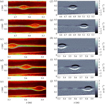
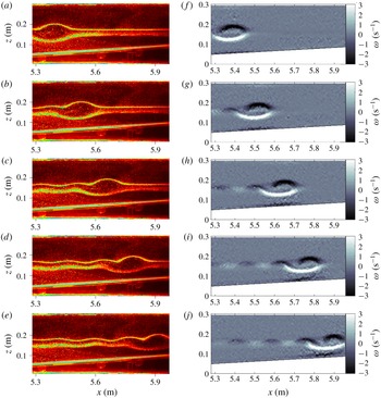
In figure 3, observations of wave propagation over the shallowest slope,
 $s=0.03$
, are presented. Figure 3(a–e) images are taken from the experimental movie, using a false-colour scheme to visualise optimally the flow field in the illuminated section. Figure 3(f–j) represents the corresponding vorticity fields as computed by PIV. The images are ordered sequentially in time from top to bottom at fixed time intervals of
 $\unicode[STIX]{x0394}t$
. Here,
 $\unicode[STIX]{x0394}t=5~\text{s}$
; in all subsequent figures
 $\unicode[STIX]{x0394}t=3~\text{s}$
unless stated otherwise. In all experiments, the incident mode-2 wave did not have a tail associated with it as it propagated over the flat bed where the upper and lower layer depths were approximately equal and the pycnocline was centred on the mid-depth of the water column. Figure 3(d,i,e,j) shows that, as the wave propagates over the slope, and as the ratio of the upper and lower layer depths varies, an oscillatory tail develops behind the mode-2 wave. Moreover, the amplitude of the wave tail becomes more pronounced (figure 3
e,j) as the mode-2 wave continues to propagate further along the slope and (i) the difference in the layer depths increases and (ii) the stratification profile becomes increasingly asymmetrical across the mid-depth.
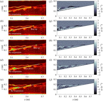
Sequence of raw images (a–e) and corresponding vorticity fields (f–j) from experiment s1a2 (
 $s=0.03,a/H=0.11$
). The time interval between panels is
 $\unicode[STIX]{x0394}t=5~\text{s}$
. Note that images are shown from two different cameras arranged horizontally to cover an integrated field of view; (a,f,b,g) camera 1, (c,h,d,i,e,j) camera 2.

Sequence of raw images (a–e) from experiment s2a2 (
 $s=0.07,a/H=0.11$
) and corresponding vorticity field (f–j). The time interval between panels is
 $\unicode[STIX]{x0394}t=3~\text{s}$
.

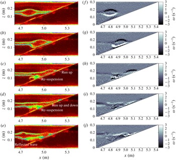
In figure 4, images are presented from the case of
 $s=0.07$
, a steeper slope than for the data shown in figure 3. In this case, the oscillatory tail is more pronounced than in the shallowest case (
 $s=0.03$
, figure 3). This is due to the ratio of the fluid layer depths changing at a quicker rate than in the previous case (figure 3) as the wave propagates up the slope. This is in keeping with the simulations of Olsthoorn et al. (Reference Olsthoorn, Baglaenko and Stastna2013) who investigated mode-2 waves propagating over a flat bed but for cases in which the ratio of the layer depths was varied parametrically. They showed that the efficiency of energy transfer from the mode-2 wave body to the oscillatory tail is enhanced with increasing asymmetry over the layer depths. The proximity to the slope of the lower interface of the wave causes the wave shape to be modified and the bottom half of the mode-2 wave to be flattened (figure 4
b,g,c,h,d,i,e,j). As the lower half of the wave is modulated by the bottom boundary in this way, asymmetry is introduced to the wave form. The asymmetry is similar to that documented in Cheng et al. (Reference Cheng, Hsieh, Hsu and Hwang2017) for mode-2 ISW propagation over slope/shelf topography (see their figure 6
a). This flow development, coupled with the presence of the oscillatory tail, causes the mode-2 wave to change form; the top interface of the wave has two peaks and the lower interface has one trough (figure 4
d,i,e,j). A similar change of form was observed by Terletska et al. (Reference Terletska, Jung, Talipova, Maderich, Brovchenko and Grimshaw2016) for mode-2 waves propagating over a step. In addition, the proximity of the mode-2 wave to the bottom boundary causes a build up of vorticity in the bottom boundary layer directly below the mode-2 wave (black signal at the lower boundary under the mode-2 wave).
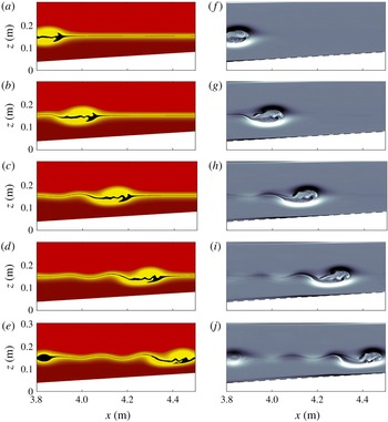
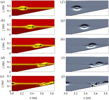
Numerical simulation of case s2a2. Panels (a–e) show the density field with a colour map created to approximate the experimental images. The densities near the centre of the undisturbed pycnocline centre have been set to black to visually accentuate this region. Panels (f–j) show the vorticity capped at
 $\unicode[STIX]{x1D714}=\pm 3~\text{s}^{-1}$
and the slope boundary is marked by a dashed grey line. The time interval between images in the sequence is
 $\unicode[STIX]{x0394}t=3~\text{s}$
. The location in the numerical domain is chosen to approximate figure 4.

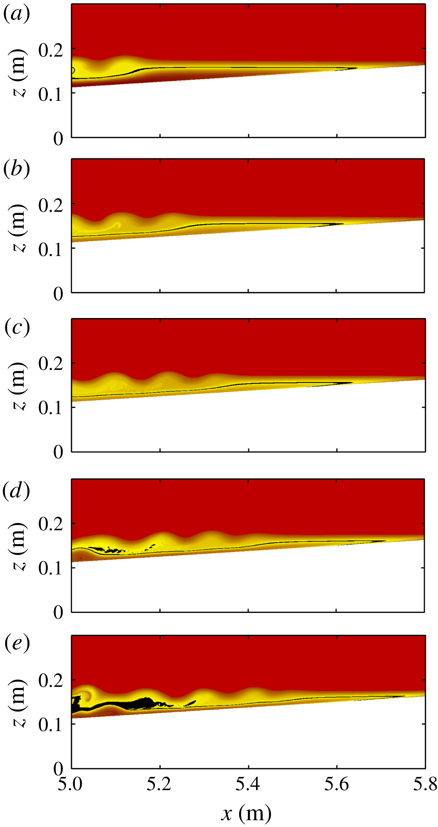
Numerical simulation of case s2a2. The density field with a colour map created to approximate the experimental images. The densities near the centre of the undisturbed pycnocline centre have been set to black to visually accentuate this region. The time interval between images in the sequence is
 $\unicode[STIX]{x0394}t=3~\text{s}$
and are chosen during the terminal shoaling portion of evolution.

In figure 5, numerical simulations that can be directly compared with figure 4 are shown. The horizontal location of the numerical simulations has been chosen to approximate that of figure 4. These two reference locations differ slightly from each other due to the manner in which the numerical model specifies the bottom topography (to maintain spectral accuracy the piecewise linear slope is smoothed). In the density plots of figure 5(a–e), fluid with a density within
 $2\,\%$
of the density at the mid-point of the undisturbed pycnocline, is darkened to illustrate the overturning core region of the leading mode-2 wave. A clear bias in fluid at this density toward the bottom half of the mode-2 wave is evident in the core. The ‘black’ interfacial fluid, is split apart asymmetrically by the propagating wave and stretched along the wave boundary. It subsequently forms cusp-like structures that rotate inward due to the vorticity (f–j) associated with the main wave body. This motion is attributed by Schmidt (Reference Schmidt1998) to an asymmetric Holmboe instability as documented for mode-2 ISWs propagating over a flat bed. In the vorticity evolution sequence (f–j), the leading mode-2 wave is clearly delineated by the spatial distribution of baroclinic vorticity. The core region exhibits considerable small scale vorticity variation. Ejection of material out of the core is evident in the density and vorticity (figures 5
d,i and 5
e,j) plots. This feature is associated with short length scale variability in the vorticity field extending behind the leading mode-2 wave body and is again in agreement with Schmidt (Reference Schmidt1998). Like the laboratory observations (figure 4), once shoaling begins, the early evolution of the mode-2 wave is marked by the formation of a clear trailing oscillatory tail. Agreement between the numerical simulation and the laboratory observations is excellent. No significant short length scale activity is observed in the bottom boundary layer.
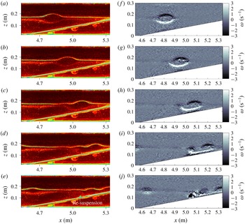
Sequence of raw images (a–e) from experiment s4a2 (
 $s=0.20$
,
 $a/H=0.11$
) and corresponding vorticity field (f–j). The time interval between panels is
 $\unicode[STIX]{x0394}t=3~\text{s}$
.

Sequence of raw images (a–e) from experiment s4a2 (
 $s=0.20$
,
 $a/H=0.11$
) and corresponding vorticity field (f–j). The time interval between panels is
 $\unicode[STIX]{x0394}t=3~\text{s}$
. The first panel (a,f) is displayed at the corresponding time to figure 7(e,j).

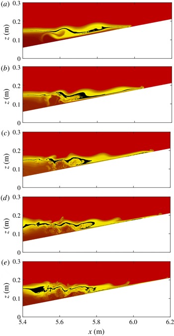
The terminal phase of shoaling and, in particular, the subsequent flow development once the pycnocline intersects the slope is shown in figure 6. (Note similar observations were not possible in the laboratory due to the limited length of the wave flume). Figure 6 has the same aspect ratio as figure 5, but has been shifted downstream. Only the density field is shown. It can be seen that the mode-2 wave degenerates into several mode-1 waves of elevation, a behaviour resembling in some respects the fission process described by Aghsaee et al. (Reference Aghsaee, Boegman and Lamb2010) for shoaling of mode-1 waves on shallow slopes. This breakdown lowers the mechanical energy density of the flow, so that the wave train effectively ‘runs out of steam’ as it moves up the slope. In contrast to the shoaling flow behaviour observed for steeper slopes (see below), little boundary layer activity is observed and there is no evidence of any reflected wave signal.
In figures 7–9 the slope steepness is increased to
 $s=0.2$
. Figures 7 and 8 are laboratory observations while figure 9 is numerical simulation. In this case, the undisturbed pycnocline intersects the slope in the laboratory observations. An oscillatory tail appears to form (see figure 7
c,h,d,i) but the time scale over which it has time to develop before the wave collides with the slope is much less than in the shallower slope cases (figures 3–5). As the wave shoals, the bottom of the mode-2 wave flattens (figure 7
c,h), vorticity is intensified at the bottom boundary, the boundary layer separates (figure 7
d,i; see figure 10 below for validation) and a vortex is generated at the bed leading to re-suspension of tracer particles from the bed (figure 7
e,j). A second mode-2 ISW (of smaller amplitude and slower speed) appears as part of the experimentally generated rank-ordered wave train and can be seen in figures 7(d,i) and 7(e,j). In figure 8 the dynamics further upstream and at later times can be seen. Panel 8(a,f) is displayed at the same time as panel 7(e,j). As the wave collides with the slope there is run up (figure 8
a,f,b,g,c,h), run down (figure 8
d,i,e,j), re-suspension and the mode-2 form of the wave is destroyed as the wave evolves into small amplitude mode-1 waves of elevation.
Figure 9 shows the numerical evolution of density and vorticity for run s4a2 and can be compared directly with the laboratory observations of figure 7. Agreement with the experimental results is again excellent. During shoaling the lower half of the mode-2 wave broadens (figure 9 c,h) and begins to lag (figure 9 d,i) the main wave. Interaction with the boundary layer occurs behind the wave as evidenced by the near-bottom swirl of density in figure 9(e). In the vorticity evolution, the main wave body is clearly marked by the distribution of baroclinic vorticity it induces. The core region exhibits considerable small scale vorticity variation. Near-bottom vorticity is largest beneath the lagging bottom half of the wave (white in vorticity panel of figure 9 i) and in the forming separation bubble (black in vorticity panel of figure 9 i) and the resulting roll up (figure 9 j).
Numerical simulation of case s4a2. Panels (a–e) show the density field with a colour map created to approximate the experimental images. The densities near the centre of the undisturbed pycnocline centre have been set to black to visually accentuate this region. Panels (f–j) show the vorticity capped at
 $\unicode[STIX]{x1D714}=\pm 3~\text{s}^{-1}$
and the slope boundary is marked by a dashed grey line. The time interval between images in the sequences is
 $\unicode[STIX]{x0394}t=3~\text{s}$
. Location in the numerical domain is chosen to approximate figure 7.

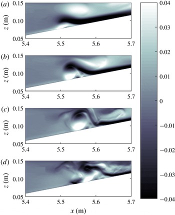
Figure 10 shows the development and bursting of the separation bubble below the shoaling wave. The figure shows the shaded horizontal velocity, as opposed to vorticity, in order to highlight the flow features. The horizontal velocity is saturated at
 $u=\pm 0.04~\text{m}~\text{s}^{-1}$
. Panels are taken every 2 s, and the initial time is chosen so that figure 10(b) corresponds to figure 9(d,i). In figure 10(a), it can be seen that the down slope flow (black) rides up and over the separation bubble (bottom white) near
 $x=5.52~\text{m}$
. The separation region subsequently grows in vertical extent, leading to vortex roll up and the generation of short length scale variations. The bottom boundary layer dynamics is similar to that observed under mode-1 ISWs of depression and are attributed to an adverse pressure gradient at the trailing edge of the wave and ‘global instability’ in the boundary layer (Bogucki, Dickey & Redekopp Reference Bogucki, Dickey and Redekopp1997; Hammond & Redekopp Reference Hammond and Redekopp1998; Stastna & Lamb Reference Stastna and Lamb2002; Diamessis & Redekopp Reference Diamessis and Redekopp2006; Carr, Davies & Shivaram Reference Carr, Davies and Shivaram2008; Boegman & Ivey Reference Boegman and Ivey2009; Boegman & Stastna Reference Boegman and Stastna2019).
Detail of the separation bubble below the shoaling wave in the numerical simulation of case s4a2. Shaded horizontal velocity saturated at
 $u\pm 0.04~\text{m}~\text{s}^{-1}$
. The time interval between panels is
 $\unicode[STIX]{x0394}t=2~\text{s}$
. Panel (b,g) corresponds to panel (d,i) in figure 9, although note the different horizontal and vertical extent of the two figures.

The numerical results corroborate the experimental observation that the shoaling mode-2 wave can induce boundary layer separation before the terminal phase of shoaling. For completeness, the terminal phase itself is shown in figure 11. Figure 11(a) is at the same time as figure 9(e,j) but the domain has been shifted in the horizontal direction to allow visualisation of where the pycnocline intersects the slope. It can be seen that the mode-2 wave breaks down into two mode-1 waves of elevation. In figure 11(c) the leading wave has broken down into a thin jet that runs up slope (cf. figures 8(c,h) and 8(d,i) from the experimental results). As the fluid in the jet begins to run down the slope, a breaking internal wave is evident (figure 11
d cf. figure 8
d,i). In MacIntyre et al. (Reference MacIntyre, Flynn, Jellison and Romero1999), the authors noted that internal waves of different modes were generated upon the cessation of winds over Mono Lake, California. These waves were observed to steepen and enhance turbulence (greatly for slopes on the order of
 $10\,\%$
) in shoaling regions. It is possible that the mechanisms observed here in the experiments and simulations could be the source of the turbulence observed in the field.
Numerical simulation of case s4a2. The density field with a colour map created to approximate the experimental images. The densities near the centre of the undisturbed pycnocline centre have been set to black to visually accentuate this region. Outputs every 3 s during the terminal shoaling portion of evolution. Panel (a) corresponds to figure 9(e,j).

Sequence of raw images (a–e) from experiment s6a3 (
 $s=0.40$
,
 $a/H=0.11$
) and corresponding vorticity field (f–j). The time interval between panels is
 $\unicode[STIX]{x0394}t=3~\text{s}$
.

Shoaling behaviour observed for different slopes.

In figure 12 the case for a slope of steepness
 $s=0.4$
is presented. In this case, as the slope is steep, there is no time for an oscillatory tail to develop before the wave collides with the slope. Like the previous case, the collision of the wave with the slope causes run up (figure 12
c,h,d,i), run down (figure 12
d,i,e,j), boundary layer separation (figure 12
b,g), vortex generation (figure 12
c,h) and re-suspension at the bed (figure 12
c,h,d,i). In this case, however, the wave does not degenerate into mode-1 waves of elevation and a reflected mode-2 wave signal is seen at later time, propagating back upstream. Note that the boundary layer vortex travels up slope but does not surpass the region of mixed fluid in the pycnocline above.
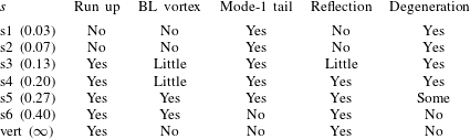
In table 2, the flow characteristics associated with shoaling for different slope steepness are summarised. It can be seen that for slope steepness,
 $s\geqslant 0.13$
, a reflected signal and significant near-bed dynamics (run up, run down, boundary layer separation and vortex formation) occur. An oscillatory tail only forms for slopes of steepness
 $s\leqslant 0.27$
; for steeper slopes there is not enough time for the tail to form before the wave collides with the slope. Moreover, the smaller the slope steepness the greater the degeneration of the wave form.
4.2 Run up
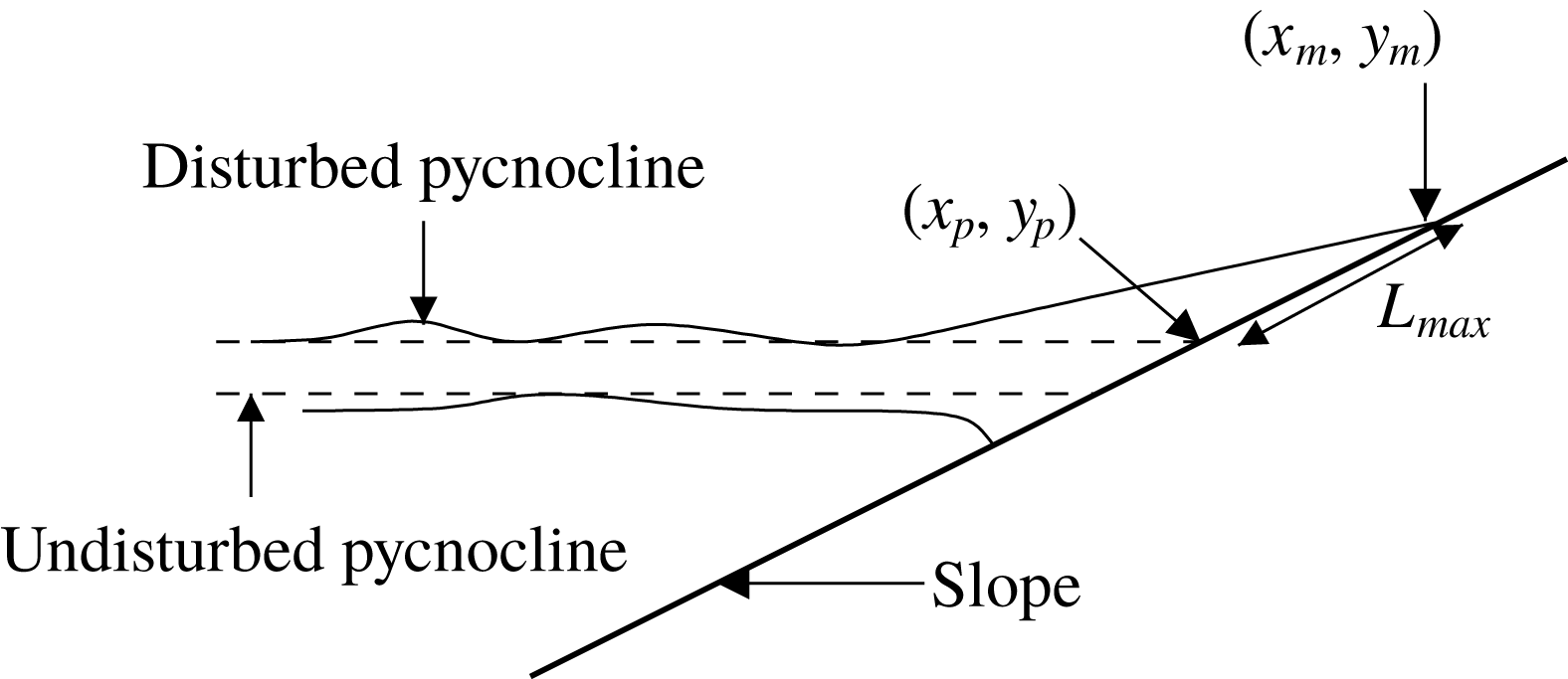
Schematic diagram to illustrate the definition of run up length
 $L_{max}$
. The dashed lines indicate the undisturbed pycnocline location.
 $(x_{p},y_{p})$
are the coordinates of the intersection of the top of the undisturbed pycnocline with the slope and
 $(x_{m},y_{m})$
are the coordinates of the highest up slope point that the run up reaches.

In cases where run up was observed in the laboratory, it was possible to measure the run up length and speed. Measurements were not possible for cases in which
 $s\leqslant 0.13$
as the maximum attained by the run up was downstream of the field of view of the cameras. Run up length was measured by tracing the top of the pycnocline and identifying the undisturbed intersection point of the top of the pycnocline with the slope (or wall in the case
 $s=\infty$
)
 $(x_{p},y_{p})$
and the location at which the run up reached a maximum
 $(x_{m},y_{m})$
(see figure 13). The run up length was defined as
 $$\begin{eqnarray}\displaystyle L_{max}=\sqrt{(x_{m}-x_{p})^{2}+(y_{m}-y_{p})^{2}}. & & \displaystyle\end{eqnarray}$$
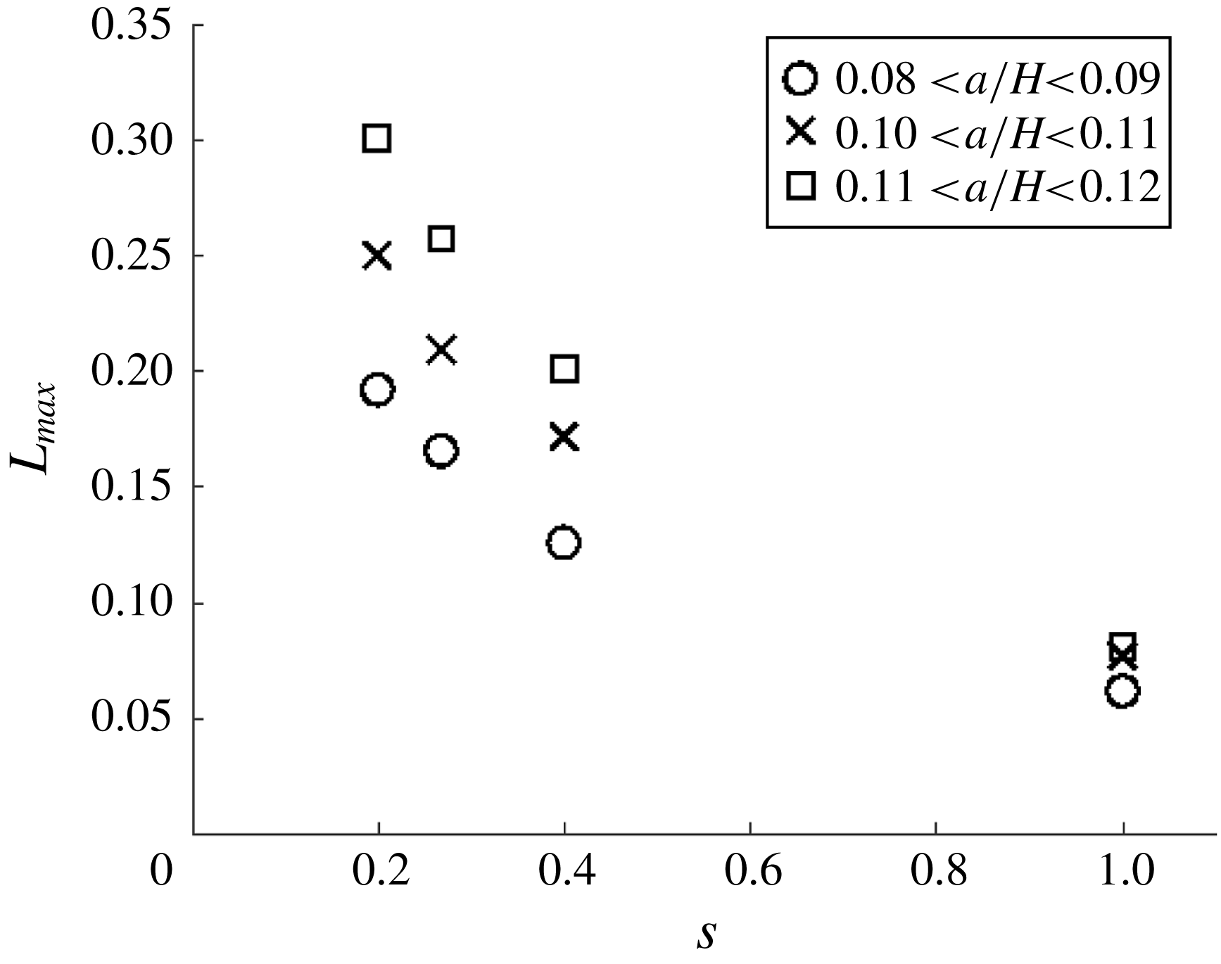
Figure 14 shows how the run up length,
 $L_{max}$
, varies with slope steepness,
 $s$
, and non-dimensional wave amplitude,
 $a/H$
. For a given wave amplitude, the run up length is reduced as the slope steepness increases. This is due to an increase in the gravitational force opposing the flow up the slope as the slope steepness increases. For a given slope steepness the run up length increases with wave amplitude. This is due to an increase in the momentum associated with an increase in wave amplitude.
Composite plot of run up length
 $L_{max}$
(m) versus slope
 $s$
for different ranges of amplitude
 $a/H$
. Different shaped symbols correspond to different values of non-dimensional wave amplitude
 $a/H$
.
 $s=1$
represents collision with a vertical wall (
 $s=\infty$
). Error bars associated with the data points are not included as they are smaller than the marker size.

Run up speed was measured from along slope time series, constructed by recording pixel intensity values along diagonal slices through images for a reference plane
 $0.002~\text{m}$
above the slope and parallel to it (Sutherland et al.
Reference Sutherland, Barrett and Ivey2013). The slices were then arranged sequentially from left to right as shown for example in figure 15. The along slope coordinate is denoted
 $x_{s}$
. In figure 15, the pycnocline (bright green patch to the left hand side) is seen to run up the slope (vertical/diagonal advancement of thin green line) before reaching a maximum height and running back down. The run up speed,
 $c_{r}$
, was computed by fitting a straight line to the portion of the time series where run up occurred and measuring the slope of the line. The run up illustrated in figure 15 was typical for all observations made i.e. the run up attained a constant up slope speed before instantaneously stopping and returning back down the slope. The bright white patch in the lower portion of the time series corresponds to resuspended particles associated with the near-bed vortex. It can be seen that this patch travels a short distance up slope but it does not pass the upper interface of the pycnocline.
Diagonal time series for case s4a2 taken along a slice parallel to the slope and
 $0.002~\text{m}$
above it. The along slope coordinate is denoted
 $x_{s}$
. The extent of the horizontal and vertical axes are
 $\unicode[STIX]{x0394}t=25.1$
s and
 $\unicode[STIX]{x0394}x_{s}=0.69~\text{m}$
respectively.

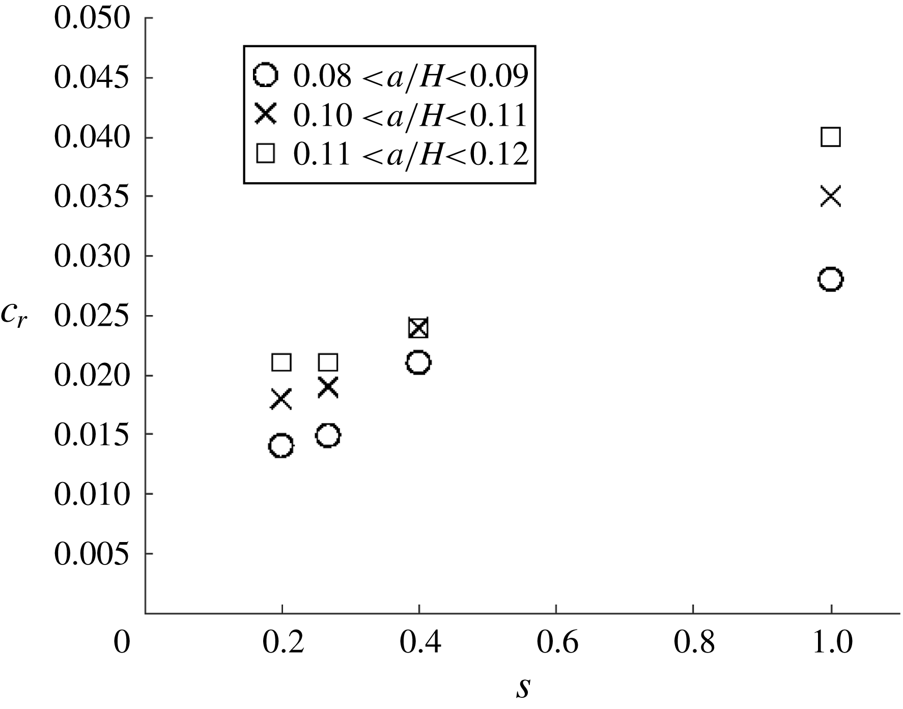
Figure 16 shows how the run up speed,
 $c_{r}$
, varies with slope steepness,
 $s$
, and non-dimensional wave amplitude,
 $a/H$
. For a given wave amplitude, the run up speed increases as the slope steepness increases. This is due to a reduction in collision time with increasing slope steepness. For a given slope steepness the run up speed increases with wave amplitude. This is due to an increase in the momentum associated with an increase in wave amplitude and is in keeping with the trend for run up length in figure 14.
Plot of run up speed (see text)
 $c_{r}$
(
 $\text{m}~\text{s}^{-1}$
) versus boundary slope
 $s$
. Different shaped symbols correspond to different values of non-dimensional amplitude
 $a/H$
.
 $s=1$
represents
 $s=\infty$
(collision with a vertical wall). Error bars associated with the data points are not included as they are smaller than the marker size.

A scaling for the maximum run up length
 $L_{max}$
of the shoaling ISW can be obtained by assuming that, at the instant of maximum run up, (i) fluid within the portion of the wave above the slope is momentarily at rest and (ii) the down slope component of the excess weight of this fluid is proportional to the incident momentum flux of the incident waves generating the run up. Such an approach has been utilised successfully by Archetti & Brocchini (Reference Archetti and Brocchini2002) and Hughes (Reference Hughes2004a
,Reference Hughes
b
) for cases of near-shore surface waves (including solitary waves) impinging on inclined beaches. For the mode-2 ISWs under consideration here, the incident momentum flux can be estimated as
 $M_{x}\approx \unicode[STIX]{x1D70C}_{2}ac^{2}W$
, of where
 $W$
is the width the channel. A proportion
 $K_{1}$
of this momentum flux is directed up the slope during shoaling such that the up slope momentum flux
 $(M_{x})_{up}\approx K_{1}\unicode[STIX]{x1D70C}_{2}ac^{2}W$
, where
 $K_{1}$
may be assumed a priori to be a function of the slope angle
 $\unicode[STIX]{x1D703}$
and the wave parameters
 $a$
and
 $c$
. When the run up length reaches its maximum value
 $L_{max}$
, the down slope component of the excess weight of the fluid in the run up current is
 $mg\sin \unicode[STIX]{x1D703}\approx K_{2}(\unicode[STIX]{x0394}\unicode[STIX]{x1D70C})(L_{max}h_{2}W)g\sin \unicode[STIX]{x1D703}$
, where the volume of run up fluid is assumed on trigonometric grounds to be proportional to
 $(L_{max}h_{2}W)$
and
 $K_{2}$
is the proportionality coefficient. Equating the net up slope momentum flux in the up slope direction with the down slope component of the excess weight (and assuming no frictional forces are significant) allows the length scale
 $L_{max}$
to be estimated from above as
 $$\begin{eqnarray}\displaystyle L_{max}\approx \frac{Kac^{2}}{g^{\prime }h_{2}\sin \unicode[STIX]{x1D703}},\end{eqnarray}$$
where
 $K(\unicode[STIX]{x1D703},a,c)=K_{1}/K_{2}$
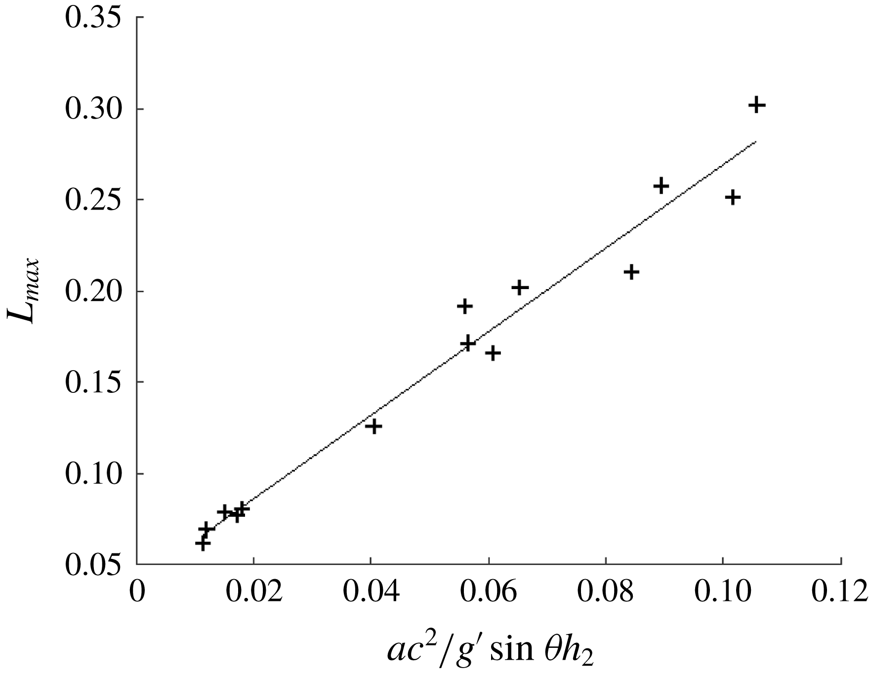
is a consolidated coefficient. In order to evaluate this scaling, the experimental run up length data are plotted in figure 17. The degree of agreement between the measured and predicted values of
 $L_{max}$
indicates that the above scaling provides a satisfactory indicator for the run up behaviour of shoaling mode-2 waves.
Run up length
 $L_{max}$
(m) versus scaling parameter
 $ac^{2}/g^{\prime }\sin \unicode[STIX]{x1D703}h_{2}$
. The solid line is the linear best fit. Error bars associated with the data points are not included as they are smaller than the marker size.

5 Discussion
5.1 Slope steepness representative of the ocean
The average angle of the continental slope is
 $2^{\circ }$
–
 $4^{\circ }$
(
 $s\in [0.03{-}0.07]$
) (Cacchione, Pratson & Ogston Reference Cacchione, Pratson and Ogston2002). The experimental observations, over slopes of this steepness, were limited by the horizontal length of the wave flume. The numerical simulations, however, may be extended in the horizontal direction with only an increase in the computation time (the resolution was fixed for all numerical experiments). In this manner a shallow slope, like that shown in figure 3 (
 $s=0.03$
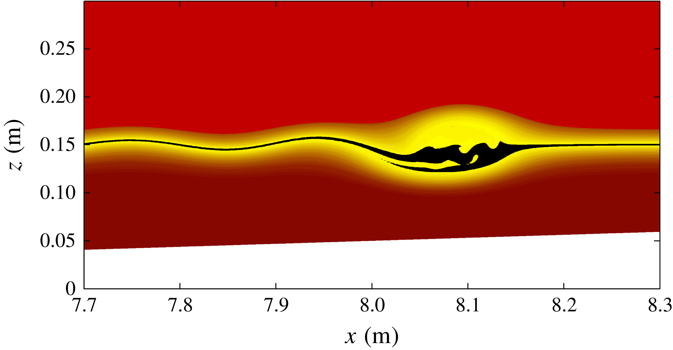
), can be considered with a domain long enough to allow the pycnocline to intersect the slope and for the terminal phase of shoaling to be observed. Figure 18 shows the numerically computed density field at a time chosen to match figure 3(e,j). It can be seen that the main mode-2 wave is slightly asymmetric across the wave crest in the horizontal direction, with a trailing oscillatory tail clearly visible.
Numerical simulation, approximation of case s1a2. The density field with a colour map created to approximate the experimental images. The densities near the centre of the undisturbed pycnocline centre have been set to black to visually accentuate this region. Output time is chosen to match the figure 3(e,j).

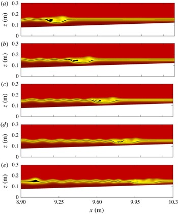
Figure 19 shows the later evolution of the shoaling mode-2 wave for the same case. The time interval between panels is
 $\unicode[STIX]{x0394}t=6~\text{s}$
. It can be seen that the evolution of the flow field is qualitatively similar to that when the slope is doubled (
 $s=0.07$
) as shown in figure 5(a–e). However, the energy transfer from the leading mode-2 wave to the trailing tail can occur over a much longer period of time (before the stratification intersects the slope). Thus the leading mode-2 wave decreases in amplitude significantly (compare figures 19
a and 19
e), and seven individual crests of the tail’s wave train are evident. The dynamics is more gentle than in cases where the slope is steeper. Inspection of the corresponding vorticity field showed some evidence of boundary layer separation but no associated vortex. Similarly, the terminal phase of shoaling (where the pycnocline intersects the slope) was gentle with very little boundary layer activity and no evidence of overturns.
Numerical simulation, approximation of case s1a2. The density field with a colour map created to approximate the experimental images. The densities near the centre of the undisturbed pycnocline centre have been set to black to visually accentuate this region. The time interval between panels is
 $\unicode[STIX]{x0394}t=6~\text{s}$
and has been chosen to show the early shoaling portion of evolution.

5.2 Viscous dissipation, bottom stress and Reynolds number
Numerical simulations allow for the exploration of fields that are difficult to obtain in the experimental setting. Three relevant examples are viscous dissipation, bottom stress and Reynolds number,
 $Re$
. The viscous dissipation is defined to be the double contraction of the rate of strain tensor multiplied by the kinematic viscosity (Kundu, Cohen & Dowling Reference Kundu, Cohen and Dowling2015). This quantity is expected to be dominated by shear near the boundaries. Nevertheless, it is interesting to see when and where substantial dissipation occurs in the fluid interior.
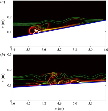
In figures 20(a) and 20(b), viscous dissipation plots are shown for the cases s4a2 and s2a2 respectively. The viscous dissipation is scaled by
 $50\,\%$
of the maximum value in the interior of the domain. This was done on a trial and error basis in order to best illustrate details of the dynamics. For the case s4a4 (figure 20
a), the time corresponding to figure 9(e,j) is shown. The subdomain is slightly shifted and reduced in size to concentrate on the flow dynamics of interest. It can be seen that the boundary layer separation at the trailing end of the mode-2 wave (which is no longer a single wave at this time) dominates the viscous dissipation. Interestingly, a second region of strong dissipation can be seen to coincide with the high shear along the bottom portion of the pycnocline. For the case s2a2 (figure 20
b), the time corresponding to figure 6(d) is shown. Again the subdomain is slightly shifted and reduced in size to concentrate on the flow dynamics of interest. This time, however, the subdomain is shifted upstream as the region in which the mode-2 wave breaks down into a wave train is not particularly energetic, with little viscous dissipation. A complex interplay between incident and reflected waves which leads to overturning and high values of the viscous dissipation can be seen. In contrast to the steeper slope case (figure 20
a), the spatial distribution of viscous dissipation is far less coherent.

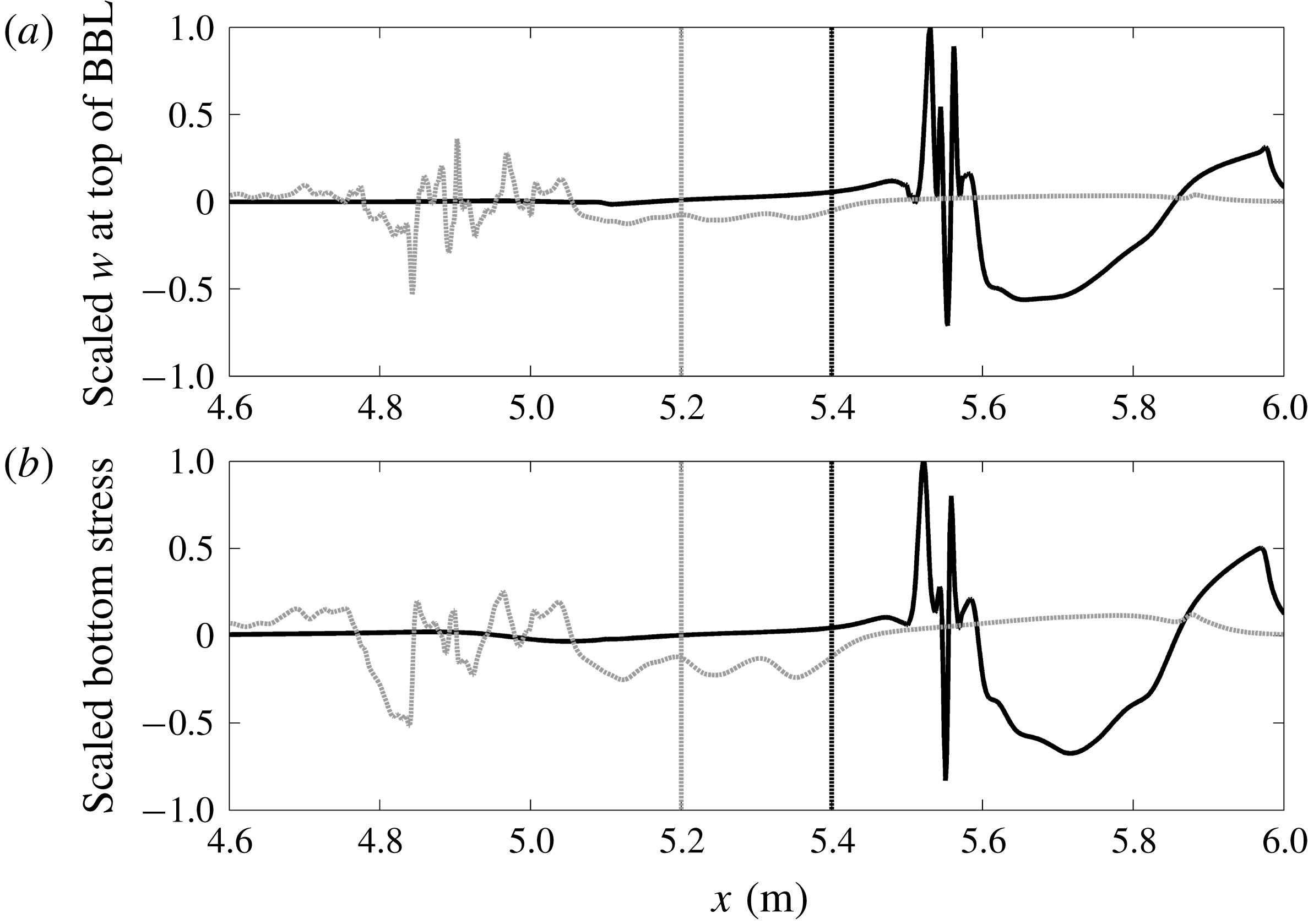
In figure 21, the vertical velocity at the top of the boundary layer and the bottom stress corresponding to figure 20 are shown for case s4a2 (black) and s2a2 (grey). The vertical velocity and bottom stress are non-dimensionalised by their maximum value which occurred in the s4a2 case for both cases. The vertical dashed lines indicate the respective extent of the domains shown in figure 20 (to the left of the grey dashed line and to the right of the black dashed line). For the case s4a2 (black), increased bottom stress is coincident with localised vertical pumping at the top of the boundary layer. Thus any resulting sediment resuspension would have a means for transport out of the bottom boundary layer region. The case s2a2 leads to instances of bottom stress at roughly
 $25\,\%$
of the s4a2 case, but this is in a region with less coherent vertical currents capable of effectively pumping any resuspended sediment out of the bottom boundary layer.
The (a) vertical velocity at the approximate top of the boundary layer and (b) bottom stress for cases s4a2 (black) and s2a2 (grey). The times correspond to figure 20. The black and grey vertical dashed lines indicate the left- and right-hand edges of the spatial domain in figures 20(a) and 20(b) respectively.

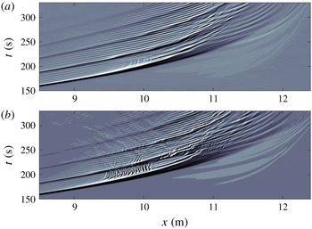
Hovmöller plot of vertical velocity
 $w$
for (a) case s1a2 and (b) case s1a2 with double
 $Re$
. The vertical velocity is saturated at
 $w=\pm 1~\text{mm}~\text{s}^{-1}$
.

In figure 22, a Hovmöller plot of vertical velocity
 $w$
at a fixed distance above the sloping bottom is shown for the case shown in figure 19, as well as a case with a doubled Reynolds number. This is achieved by halving the numerical value of the viscosity in the simulations. The thickness of the boundary is adjusted for by using the standard
 $\sqrt{Re}$
scaling from flat plate boundary layer theory. This is not exact for the case of shoaling ISWs, however the conclusions based on the figure are unchanged as the precise height above the bottom is varied. It can be seen that the Reynolds number affects the bottom boundary layer dynamics and, in particular, higher
 $Re$
results in higher vertical velocities that occur in spatio-temporal bursts characterised by shorter length scales. Note that variation in
 $Re$
did not significantly change the wave form during the shoaling process. However, cross benthic boundary layer (BBL) transport could be fundamentally different; for example see
 $9.5~\text{m}<x<10.0~\text{m}$
and
 $180~\text{s}<t<205~\text{s}$
. This suggests that when scaling up to the field scale for which
 $Re$
is large, some aspects of the bottom boundary layer dynamics seen in the steeper slope cases may be replicated in the shallow slope cases.
6 Conclusions
The characteristics of mode-2 ISWs shoaling on linear, uniform slopes have been investigated. For slope angles representative of values in the ocean, namely
 $2^{\circ }$
–
 $4^{\circ }$
, (
 $s\in [0.03,0.07]$
) the waves dissipate energy as they shoal by (i) forming an oscillatory tail and (ii) evolving into forward propagating mode-1 waves of elevation. The waves are effectively destroyed by the shoaling process and no reflected energy is expected to be seen for slope steepness representative of the ocean. The boundary layer dynamics in these cases appears to be negligible compared to steeper slopes but evidence of flow separation aft of the wave was seen (figure 5
i,j) and analysis of the Reynolds number (§ 5.2) suggests that significant boundary layer activity (akin to the steeper slope cases) is possible in the field. For steeper slopes, in addition to boundary layer separation, an associated vortex formed at the bed; it propagated up slope and was capable of resuspending material from the bed. These features are in keeping with the field observations of Bogucki, Redekopp & Barth (Reference Bogucki, Redekopp and Barth2005), who document both flow reversal in the near-bottom current just after a mode-2 ISW has passed and vertical near-bed structure suggestive of a vortex. The observations of Bogucki et al. (Reference Bogucki, Redekopp and Barth2005) were made at the Middle Atlantic Bight on the continental shelf where the slope steepness (
 $s\approx 0.001$
) is significantly less than those investigated here. The boundary layer dynamics is similar to that seen under shoaling mode-1 ISWs (Boegman & Ivey Reference Boegman and Ivey2009; Aghsaee et al.
Reference Aghsaee, Boegman, Diamessis and Lamb2011; Boegman & Stastna Reference Boegman and Stastna2019) and large amplitude mode-1 ISWs of depression propagating over a flat bed (Bogucki et al.
Reference Bogucki, Dickey and Redekopp1997, Reference Bogucki, Redekopp and Barth2005; Stastna & Lamb Reference Stastna and Lamb2002; Diamessis & Redekopp Reference Diamessis and Redekopp2006; Carr et al.
Reference Carr, Davies and Shivaram2008). The dynamics is attributed to an adverse pressure gradient under the rear of the wave and global instability (Bogucki et al.
Reference Bogucki, Dickey and Redekopp1997; Hammond & Redekopp Reference Hammond and Redekopp1998). Moreover, boundary layer separation and vortex formation have been shown, in the mode-1 literature, to be dependent on the Reynolds number of the flow. This is in keeping with the analysis for the mode-2 wave-induced BBL flow presented here (see § 5.2).
While similarities are seen in the BBL dynamics beneath shoaling mode-1 ISWs, differences (not unexpectedly) are seen when comparing the evolution of the waveform. In the mode-1 case, different kinds of wave breaking (spilling, plunging, surging and collapsing) have been documented as the wave shoals, see for example Sutherland et al. (Reference Sutherland, Barrett and Ivey2013) and references therein. The dynamics of the shoaling mode-1 waves was characterised by the Iribarren number,
 $Ir=s/\sqrt{a/2\unicode[STIX]{x1D706}}$
, which measures the ratio of the topographic slope to the square root of the characteristic wave slope. In table 1 measures of
 $Ir$
and wave steepness
 $a/\unicode[STIX]{x1D706}$
are provided to allow comparison. Wave steepness was approximately constant
 $a/\unicode[STIX]{x1D706}\in [0.39,0.50]$
due to the linear relationship between wave amplitude and wavelength (Schmidt Reference Schmidt1998). The Iribarren number, however, had a range
 $Ir\in [0.07,0.90]$
. Despite this, the mode-2 waves studied here evolved into mode-1 waves of elevation as they shoaled and they developed a mode-1 tail. For gentle slopes (
 $s\leqslant 0.07$
) the vast majority of the wave energy was dissipated in this way, while in steeper cases some energy went into BBL effects, wave run up, run down and reflection back off the slope. Another noticeable difference between shoaling mode-1 and shoaling mode-2 ISWs is that no boluses are formed in the mode-2 case. Helfrich (Reference Helfrich1992) and Arthur & Fringer (Reference Arthur and Fringer2014) have shown that shoaling mode-1 ISWs can create boluses that propagate up slope. Evidence of this in the field (Hosegood & van Haren Reference Hosegood and van Haren2004) has shown that mass and energy can be transported significant distances shoreward away from the pycnocline from shoaling ISWs. In the case of mode-2 ISWs (which are significantly less energetic than mode-1 ISWs), the results presented here suggest that dissipation of energy in the shoaling process is much more localised than in the mode-1 case. This may have significant implications with nutrients and core material from mode-2 ISWs being expected to be deposited in localised shoaling regions on the continental shelf. This area of study would benefit from field observations and an assessment of bottom roughness.
Acknowledgements
The authors are grateful for support from the University of Dundee and for technical assistance provided by J. Anderson and D. Turbyne (University of Dundee). The authors thank two anonymous referees for critical comments that have improved the paper.