
1 Introduction
There are several instabilities that can cause transition in a three-dimensional boundary layer including the centrifugal, streamwise and cross-flow instabilities. The cross-flow instability can occur on different configurations such as swept wings, cylinders, rotating disks and cones at angle of attack (Saric, Reed & White Reference Saric, Reed and White2003). On a cone at angle of attack in hypersonic flow, the bow shock is not axisymmetric, creating a circumferential pressure gradient. This pressure gradient generates curved streamlines within the boundary layer by providing a centripetal force, thinning the windward boundary layer and thickening the leeward boundary layer (Li et al. Reference Li, Choudhari, Chang and White2010; Schuele Reference Schuele2011).
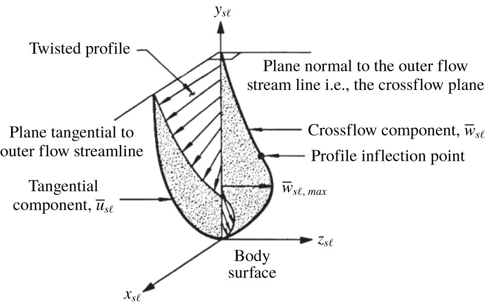
Within the boundary layer, pressure is approximately constant in the wall-normal direction. Velocity is zero at the wall due to the no-slip condition and the spanwise velocity (perpendicular to the inviscid streamline) is also zero at the boundary-layer edge. These two velocity boundary conditions result in a spanwise velocity profile with an inflection point, as seen in figure 1 (Adams & Martindale Reference Adams and Martindale1973). This inflection point provides a source of an inviscid instability, which leads to the development of stationary and/or travelling cross-flow vortices that can lead to transition to turbulence (Saric et al. Reference Saric, Reed and White2003).
Boundary-layer profiles illustrating inflection point arising from pressure-gradient-induced cross-flow (Adams & Martindale Reference Adams and Martindale1973).

In general, ‘stability analysis’ refers to a method of decomposing a Navier–Stokes solution into two parts; an unperturbed ‘basic state’ and a perturbation on this solution. One can then formulate a set of equations, which depend heavily on leveraging the assumptions made about the basic state quantities, which form a complex eigenvalue problem having complex exponential solutions. All the methods in this family are derived by inserting the decomposed flow variables into the full Navier–Stokes equations and simplifying by truncating small terms. A fallout of the simplifications made is that the disturbances typically take the form of sinusoidal waves in time and the non-resolved (homogeneous) spatial directions. In this context, linear stability theory (LST) assumes only one non-homogeneous direction (wall normal). Both linear and nonlinear parabolized stability equations (PSE) assume one rapidly varying non-homogeneous direction, as in LST, but add the assumption of a second ‘slowly varying’ non-homogeneous direction to account for streamwise development of the disturbance. The PSE can be solved linearly (single disturbance) or nonlinearly (accounting for multiple disturbances and their interactions).
Computational work pertaining to the cross-flow instability has focused on modelling the stability and receptivity of three-dimensional boundary layers using a variety of computational tools including LST, PSE and direct numerical simulation (DNS). Each of these techniques have different advantages. LST analyses offer the simplest and least computationally intensive approach, but they ignore nonlinear and non-parallel effects (Malik & Balakumar Reference Malik and Balakumar1992). These assumptions can lead to discrepancies between computed predictions and experimental results. PSE can take into account nonlinear and non-parallel effects, thus more accurately predicting the transition process (Chang et al. Reference Chang, Malik, Erlebacher and Hussaini1993; Kuehl, Perez & Reed Reference Kuehl, Perez and Reed2012; Kuehl Reference Kuehl2016). DNS simulates the fully nonlinear governing equations, thus providing the most detailed results with the least number of assumptions (Dinzl & Candler Reference Dinzl and Candler2017). This technique, however, requires substantial computational power.
The Langley Stability and Transition Analysis Code implements LST and PSE to predict transition on two-dimensional, axisymmetric and infinite swept-wing boundary layers (Chang Reference Chang2003). They validated the code for several configurations including Mach-2 flow over a flat plate, Mach-6 flow over a compression cone and Mach-2 flow over a swept wing with roughness control. They concluded that transition N-factor correlation remains the most viable option for transition prediction. Li et al. used LST and PSE to study transition over a circular cone at  $3^{\circ }$ and
 $6^{\circ }$ angle of attack at Mach 6 (Li et al. Reference Li, Choudhari, Chang and White2010). The computations were modelled to match the corresponding experimental conditions in the Boeing/AFOSR Mach-6 Quiet Tunnel (BAM6QT) at Purdue University. Two configurations were studied: flow over a yawed circular cone and flow over a compression cone. The maximum stationary cross-flow N-factors were computed along streamline trajectories and found to be between 10 and 20. These N-factors provided assessments of predicted transition fronts and disturbance characteristics, including frequency content and wavenumbers.
Balakumar and Owens studied the stability characteristics on a cone at angle of attack in hypersonic flow using DNS to solve the three-dimensional Navier–Stokes equations in cylindrical coordinates (Balakumar & Owens Reference Balakumar and Owens2009). Simulations were conducted at Mach 6 at nominally identical free-stream conditions compared to experiments in the BAM6QT. Simulations containing between 30 and 70 stationary cross-flow vortices were performed by modelling roughness elements on the simulated cone. N-factor computations predicted transition would occur more rapidly on the yaw side of the cone (between the windward and leeward rays), with the earliest transition detection occurring at  $\unicode[STIX]{x1D719}=110^{\circ }$. The wavenumbers of the stationary cross-flow vortices evolved as the vortices progressed downstream.
Regardless of the chosen technique, previous computational works modelling the stationary cross-flow vortices have relied on seeding initial disturbances on the computational grid in order to excite disturbances at a characteristic wavelength (Dinzl & Candler Reference Dinzl and Candler2017). While arbitrarily spaced disturbances can successfully excite disturbances of a given wavenumber, connecting the wavenumber of the controlled disturbance input to the wavenumber of instabilities at transition is not straightforward because the local wavenumber varies as the disturbances evolve downstream (Moyes et al. Reference Moyes, Kocian, Mullen and Reed2017). An open question in the research community, therefore, is how to accurately predict the wavenumber of the largest amplitude disturbances.
Previous research efforts using the PSE method on conical geometries have attempted to more accurately model the spatial evolution of the wavenumber of the stationary cross-flow waves by holding the total number of waves constant and adjusting the local wavenumber based on the local geometric circumference. In this approach, the wavenumber is assumed to be uniform azimuthally, but varies axially. While this assumption partially accounts for the spatial evolution of the wavenumber, it does not fully capture the spatial evolution of the largest amplitude stationary waves. Recently, more robust computational techniques have been implemented to address this challenge. Kuehl et al. proposed a technique to account for the local wavenumber variations in the marching direction of their stability analysis conducted on a yawed circular cone (Kuehl et al. Reference Kuehl, Perez and Reed2012). This method relied on the assumption that the evolution of wavenumber was a function of radius of curvature. Because the local streamlines are inclined relative to a constant azimuth, the local radius of curvature was taken to be an effective radius in the wall-normal direction. This technique required an assumption of the initial wavenumber where the disturbances were seeded. Moyes et al. refined the computational technique of Kuehl et al. to compute the local effective wavenumber and implemented this on the HiFIRE-5 elliptic cone geometry (Moyes et al. Reference Moyes, Kocian, Mullen and Reed2017). Moyes et al. proposed an adjustment to the basic state to model the evolution of wavenumber measured in the direction perpendicular to the marching path (in this case taken along a cross-flow vortex path). This methodology assumed that the number of waves remained constant in the space between the arbitrarily seeded computational vortex paths. As the paths moved along the cone, the distance between paths, measured in azimuthal angle, could increase or decrease. This change in spacing, along with the local orientation of the disturbance path, was used to determine what the local effective wavenumber would be (Moyes et al. Reference Moyes, Kocian, Mullen and Reed2017). While these techniques more accurately modelled the changes in local wavenumber as the disturbances progressed downstream, they still cannot predict the actual wavenumber of the stationary cross-flow waves that would be observed experimentally or in flight.
In this work, a new technique is presented to more accurately model the spatial wavenumber evolution of the largest amplitude stationary cross-flow waves. The local wavenumbers are computed from experimental data, providing greater insight into the boundary-layer physics and resulting in a more robust computational approach. The local wavenumbers of the vortices are extracted from experimental observations of stationary waves, taken on a yawed circular cone under quiet-flow conditions at Mach 6 in the BAM6QT. The experimental wavenumbers are computed via a wavelet analysis of the surface heating distribution, which captures the axial and azimuthal wavenumber variation. The wavenumbers of the stationary waves with the local largest amplitude are thereby obtained. The stability analysis then computes N-factors by integrating the local amplification rate along computed vortex paths corresponding to the largest amplitude wavenumbers observed in the experiment. This method is advantageous compared to previous techniques because it directly measures the evolution of the disturbance wavenumbers. Additionally, a second stability analysis is conducted, implementing a computational technique based on vortex path spreading similar to the work of Moyes et al. This technique yields a non-dimensional wavenumber ratio, seeking to more accurately predict the spatial wavenumber variation of the stationary cross-flow waves. The results are dimensionalized by the experimental data for each respective path. Finally, the stability analysis is conducted using the computationally predicted most unstable wavenumbers.
2 Experiment
2.1 Test model
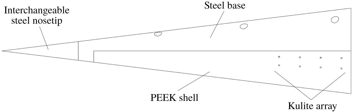
A  $7^{\circ }$ half-angle circular cone was used in the experiments (figure 2). The model was manufactured from 304 stainless steel and polyether ether ketone (PEEK). The nose tip and frustum base were both constructed from stainless steel. The shell was constructed from PEEK in order to obtain global temperature maps on this section of the model using infrared (IR) thermography. PEEK, which has a high emissivity and low thermal conductivity, is well suited for IR thermography (Hirschen & Gülhan Reference Hirschen and Gülhan2009; Willems et al. Reference Willems, Gülhan, Juliano, Kimmel and Schneider2014). Overall, the model was 413.5 mm long with a 101.6 mm base diameter. This was the maximum size that could be reliably started in the facility at the relevant angles of attack. In these experiments, a stainless steel nose tip with a 1.0 mm nose diameter was used. The model configuration was designed to observe the unperturbed evolution of the stationary cross-flow waves, thus providing data on the largest amplitude wavenumbers. The root mean square (r.m.s.) surface roughness of the nose tip was measured 20 mm from the stagnation point, which was near the neutral points of the stationary waves, using an Olympus LEXT OLS4100 Confocal Microscope and found to be
 $0.81~\unicode[STIX]{x03BC}\text{m}$ with
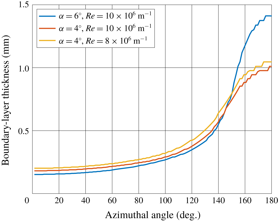
 $\pm 0.01~\unicode[STIX]{x03BC}\text{m}$ uncertainty. The boundary-layer thickness was computed (see § 3) as a function of azimuthal angle at this axial station for different angles of attack,
 $\unicode[STIX]{x1D6FC}$, and different Reynolds numbers (figure 3). The thinnest boundary layer at the
 $x=20~\text{mm}$ station is 0.15 mm (
 $\unicode[STIX]{x1D719}=0^{\circ }$,
 $\unicode[STIX]{x1D6FC}=6^{\circ }$,
 $Re=10\times 10^{6}~\text{m}^{-1}$). The ratio of the measured r.m.s. surface roughness to the computed boundary-layer thickness is
 $5.4\times 10^{-3}$.
Test-model schematic.

Boundary-layer thickness for different flow conditions at  $x=20~\text{mm}$.

2.2 Boeing/AFOSR Mach 6 Quiet Tunnel
The experimental data were collected in the BAM6QT at Purdue University. The tunnel is a Ludwieg tube design, which was chosen to minimize cost while achieving fairly high free-stream Reynolds numbers (Schneider Reference Schneider2008). This design utilizes a long driver tube, followed by a converging–diverging nozzle that accelerates the flow to the designed Mach number, and finally a vacuum tank at the downstream end of the tunnel.
For this work, the BAM6QT ran under quiet-flow conditions. The tunnel is capable of achieving quiet-flow free-stream pressure fluctuations of less than 0.02 % of the mean pressure through several design features. The tunnel nozzle is polished to a mirror finish to inhibit roughness-induced boundary-layer transition. In the contraction section of the nozzle, a suction slot removes the boundary layer growing at this axial location of the tunnel. A valve allows the bleed air to bypass the diverging nozzle and test section to feed directly to the vacuum tank. A new laminar boundary layer then begins to form downstream of this location (Chynoweth Reference Chynoweth2015). This feature removes tunnel-wall boundary-layer fluctuations that could lead to a turbulent wall boundary layer in the test section (Juliano, Schneider & Aradag Reference Juliano, Schneider and Aradag2008).
3 Mean-flow computational methods and results
Computations were conducted to predict the heating rates for fully laminar and fully turbulent boundary-layer state at the test conditions. These results gave confidence in the experimental data-acquisition techniques. The Overflow2.2n flow solver, using third-order accurate HLLE++ fluxes, was used to solve unperturbed, steady Navier–Stokes solutions. For both the laminar heat-flux calculations and mean-flow solutions to be used in later stability calculations, no turbulence models were needed. For the turbulent heat-flux calculations, the Spallart–Allmaras model (SA-noft2) with default coefficients was used over the entire geometry. For all cases, the flow was solved as a steady-state flow. Boundary conditions for the model surfaces were modelled as no-slip, isothermal, uniform-temperature walls. Flow conditions were selected to model conditions as run in the BAM6QT. These conditions are summarized in table 1, where  $Re$ is the free-stream unit Reynolds number,
 $L$ is the model length,
 $\unicode[STIX]{x1D70C}_{\infty }$,
 $p_{\infty }$,
 $T_{\infty }$ and
 $M$ are the free-stream density, pressure, temperature and Mach number,
 $T_{w}$ is the wall temperature and
 $T_{0}$ is the stagnation temperature. In this work, the free-stream unit Reynolds number is defined as
 $Re_{x}/x$, where
 $Re_{x}$ is the length Reynolds number defined as
 $u_{\infty }x/\unicode[STIX]{x1D708}_{\infty }$. Here,
 $u_{\infty }$ and
 $\unicode[STIX]{x1D708}_{\infty }$ are the free-stream velocity and kinematic viscosity, respectively and
 $x$ is the distance from the nose tip.
Nominal wind-tunnel flow parameters.

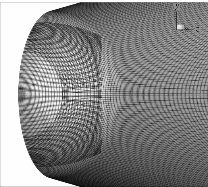
Structured, hexahedral, multi-block overset grids were created using an in-house Fortran program. Connectivity and grid metric data were computed using Pegasus 5.2. The computational model’s surface was completely smooth (no modelled surface roughness) with a spherical tip. The nose was represented by projecting a square mesh onto the sphere and subsequently smoothing the projected shape to blend smoothly with a conical grid placed on the frustum.
The computational domain covers only a half-cone ( $180^{\circ }$ azimuthal extent) to reduce computational expense, while allowing for the addition of angle of attack. From the surface, the domain extends to capture the full shock. Additional overset grids were added to the system to better refine the shock after an initial solution was calculated. For both computational and experimental data the
 $x$-axis (axial distance) is defined as positive along the streamwise direction. The
 $y$-axis is defined such that the windward ray is negative
 $y$, and the
 $z$-axis is the cross-product. Azimuthal angle is defined as
 $\text{arctan}(z,y)+180^{\circ }$ such that the windward ray is located at an azimuthal angle of
 $0^{\circ }$.
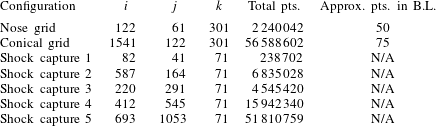
Grid resolution details are summarized in table 2. In table 2,  $i$ represents axial (
 $\pm x$),
 $j$ represents azimuthal points, while
 $k$ represents wall normal. The surface grid topology at the overlapped nose can be seen in figure 4. Wall-normal spacing in terms of
 $y^{+}$ was a maximum of 0.8 anywhere on the surface of the cone for the worst case (
 $6^{\circ }$ angle of attack, turbulent).
Surface grid topology at nose.

Grid resolution details (one half-cone).

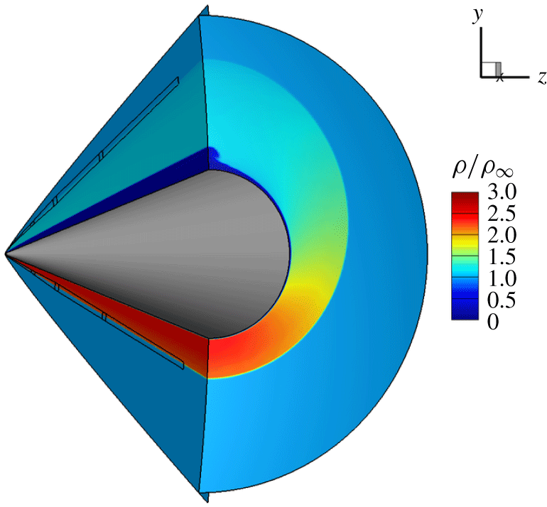
An overview of the computational domain and contours of density for Case 1 can be seen in figure 5. The lines present on the symmetry plane show the location of the additional shock-capture grids. One can see the difference in shock angle from windward to leeward that causes the circumferential pressure gradient. Note also the ‘mushroom’ flow feature and associated boundary-layer thickening that begins at  $160^{\circ }$ of azimuth near the leeward ray. The influence of this flow feature is apparent in many later results.
Non-dimensional density contours.

Surface heat flux, Case 1 flow conditions, fully laminar flow.

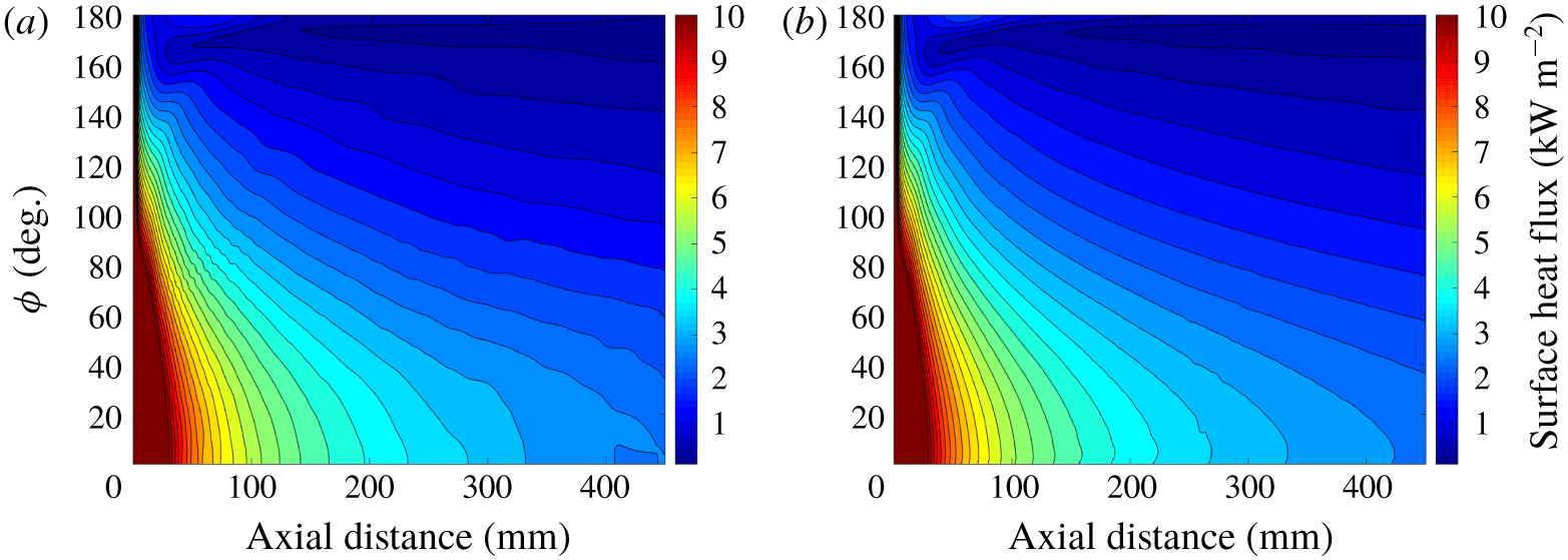
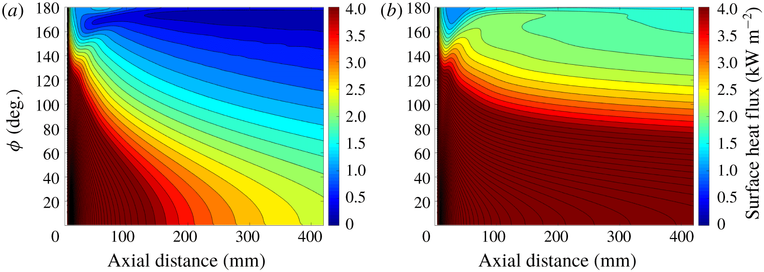
Figure 6 plots contour lines of heat flux at  $6^{\circ }$ angle of attack and nominal wind-tunnel conditions calculated with the fine and coarse grids. The largest changes are near the leeward ray, far downstream. The grids used for calculations in the current study are judged to be sufficient based on convergence of the surface heat transfer. Global heat-flux maps were constructed from the mean-flow computational results. Figure 7 shows the computational laminar and turbulent surface heating rates for Case 1 (recall table 1). These conditions are nominally identical to the baseline experimental conditions. As will be done when presenting experimental data, the colour bar scale for this figure has been chosen to more easily see variation in heat-flux data over the primary region of interest (where cross-flow is the dominant instability mechanism). The boundary layer grows downstream, and the circumferential pressure gradient causes the boundary layer to grow towards the leeward ray. For these reasons, heat flux decreased axially downstream and azimuthally towards the leeward ray. The boundary layer separates along a line near the leeward ray (
 $\unicode[STIX]{x1D719}\approx 165^{\circ }$) (Balakumar & Owens Reference Balakumar and Owens2010). This behaviour results in heating rates being lowest near the leeward ray for both the laminar and turbulent cases. The turbulent heating rates are up to five times greater than the laminar heating rates. The mean-flow computations do not convey the development of the stationary cross-flow vortices because they begin at a very low initial amplitude in the model. The mean-flow computations also assume that there is no surface roughness and that the free stream is quiescent. The simulations are run non-time accurate, therefore there is no instability growth in the model.
Computational heat flux. Case 1 flow conditions.

4 Experimental data reduction
4.1 Infrared camera and heat-flux calculation
The surface temperature of the PEEK shell was measured with an InfraTec 8300 hp IR camera. This is a 14-bit camera with a mid-wave spectral range of  $2.0{-}5.5~\unicode[STIX]{x03BC}\text{m}$. The detector format is
 $640\times 512$ pixels. Images were acquired at 355 Hz with a wide angle lens having a focal length of 12.5 mm and field of view of
 $43.0\times 32.9$ degrees. The camera was mounted on the right (north) side of the BAM6QT, with flow moving from right to left. The viewing angle of the camera was approximately
 $10^{\circ }$ from perpendicular to the model axis. A calcium fluoride (
 $\text{CaF}_{2}$) window was used because of its transmission range of
 $0.15{-}9.0~\unicode[STIX]{x03BC}\text{m}$.
Surface heat-flux maps were calculated for the different test cases by inputting calibrated infrared temperature traces into the QCALC subroutine written by Boyd and Howell (Boyd & Howell Reference Boyd and Howell1994) (and later translated into MATLAB (Juliano, Adamczak & Kimmel Reference Juliano, Adamczak and Kimmel2014)). These traces were corrected for directional emissivity effects arising from the viewing angle of the camera. The code calculates the surface heat flux as a function of time from the temperature history at a point by numerically solving the transient one-dimensional (1-D) heat equation using a second order Euler-explicit finite difference approximation in Cartesian, cylindrical or spherical coordinates. An adiabatic, isothermal, or time-varying back-face boundary condition can be chosen. QCALC was run independently for each pixel, treating its temperature history, as measured by the infrared camera, as the front-face boundary condition. Each frame was registered to within  $1/100$ pixel accuracy of a reference image. The images were also mapped to a
 $x-\unicode[STIX]{x1D719}$ coordinate system based on an image processing code before input into QCALC (Running et al. Reference Running, Thompson, Juliano and Sakaue2017). For these tests, each point was solved in cylindrical coordinates, and the local wall thickness and radius of curvature was taken into account. An isothermal back-face boundary condition was assumed, based on an initial pre-run temperature distribution measured by the IR camera. The facility experiences approximately 200 ms of steady conditions in between reflections of the expansion wave within the driver tube and an overall run time of approximately 5 s. The combination of a short run time and thick model wall (
 ${\approx}20{-}25~\text{mm}$) meant the calculated surface heat flux was rather insensitive to the back-face boundary condition. The material properties of PEEK, used in the testing and data analysis, are given in table 3. In this 1-D analysis, spanwise and streamwise conduction were neglected. Constant and homogeneous material properties were assumed.
There are several sources of uncertainty in the surface temperature and corresponding heat flux. The IR camera measures raw intensity values, which are converted to surface temperature using the factory calibration curve for the wide-angle lens. Running observed that the surface temperature computed by the camera software was within 0.20 % of that measured with a surface thermocouple when the model’s emissivity and the transmissivity of the IR window were taken into account (Running, Sakaue & Juliano Reference Running, Sakaue and Juliano2019). In this work, the factory calibration was used to convert from raw intensity to surface temperature data, taking into account the transmissivity,  $\unicode[STIX]{x1D70F}$, of the
 $\text{CaF}_{2}$ IR window and the directional emissivity,
 $\unicode[STIX]{x1D716}_{n}$ of the model. The transmissivity of
 $\text{CaF}_{2}$ was taken to be 0.94. In the spectral range of the camera of
 $2.0{-}5.5~\unicode[STIX]{x03BC}\text{m}$, this value will vary by less than
 $\pm 0.01$. This results in a temperature uncertainty of
 $\pm 0.04\,\%$. The directional emissivity of PEEK can also introduce uncertainty into the temperature calculations of the camera. Cerasuolo found that PEEK has a nearly constant directional emissivity of 0.91 for low viewing angles, with the value rapidly decreasing past
 $80^{\circ }$ (Cerasuolo Reference Cerasuolo2016). All data presented in this work were collected where the directional emissivity was relatively constant. Because directional emissivity was a near-constant value at most viewing angles, small errors in viewing angle would negligibly impact this parameter.
The surface temperature on the model was converted to heat flux using QCALC. Additional sources of uncertainty were introduced in this process. QCALC solves the 1-D heat equation, neglecting lateral conduction. The thermal conductivity,  $k$, density,
 $\unicode[STIX]{x1D70C}$, and specific heat capacity,
 $c_{p}$, of PEEK were taken to be
 $0.29~\text{W}~\text{m}^{-1}~\text{K}^{-1}$,
 $1300~\text{kg}~\text{m}^{-3}$ and
 $1026~\text{J}~\text{kg}^{-1}~\text{K}^{-1}$, respectively (Running et al. Reference Running, Thompson, Juliano and Sakaue2017). Reported values give a maximum range for these parameters of
 $\pm 10\,\%$,
 $\pm 1.5\,\%$,
 $\pm 3.1\,\%$, respectively (van der Vegt Reference van der Vegt1999). Taking into account this variation gives a maximum heat-flux uncertainty of
 $\pm 28~\text{W}~\text{m}^{-2}$. The uncertainty of the transmissivity of the IR window gives a maximum heat-flux uncertainty of
 $\pm 12~\text{W}~\text{m}^{-2}$. The IR camera has an accuracy and resolution of
 $\pm$1.0 K and 0.02 K, respectively (Infratech 2016). This results in a maximum surface temperature uncertainty of
 $\pm 0.33\,\%$ and a corresponding maximum heat-flux uncertainty of
 $\pm 130~\text{W}~\text{m}^{-2}$. This was the primary source of uncertainty, which was approximately 15 % of the lowest laminar heating rates observed along the hot streaks at the lowest Reynolds number test case (
 $Re=5.4\times 10^{6}~\text{m}^{-1}$).
Thermal properties of PEEK.

4.2 Transition location assessment
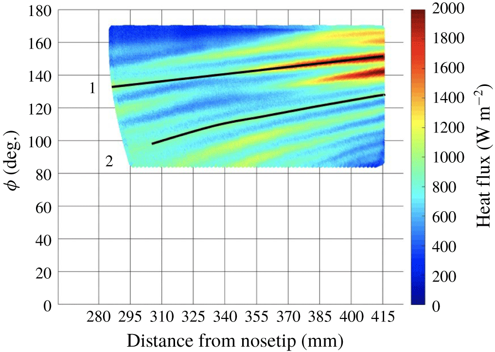
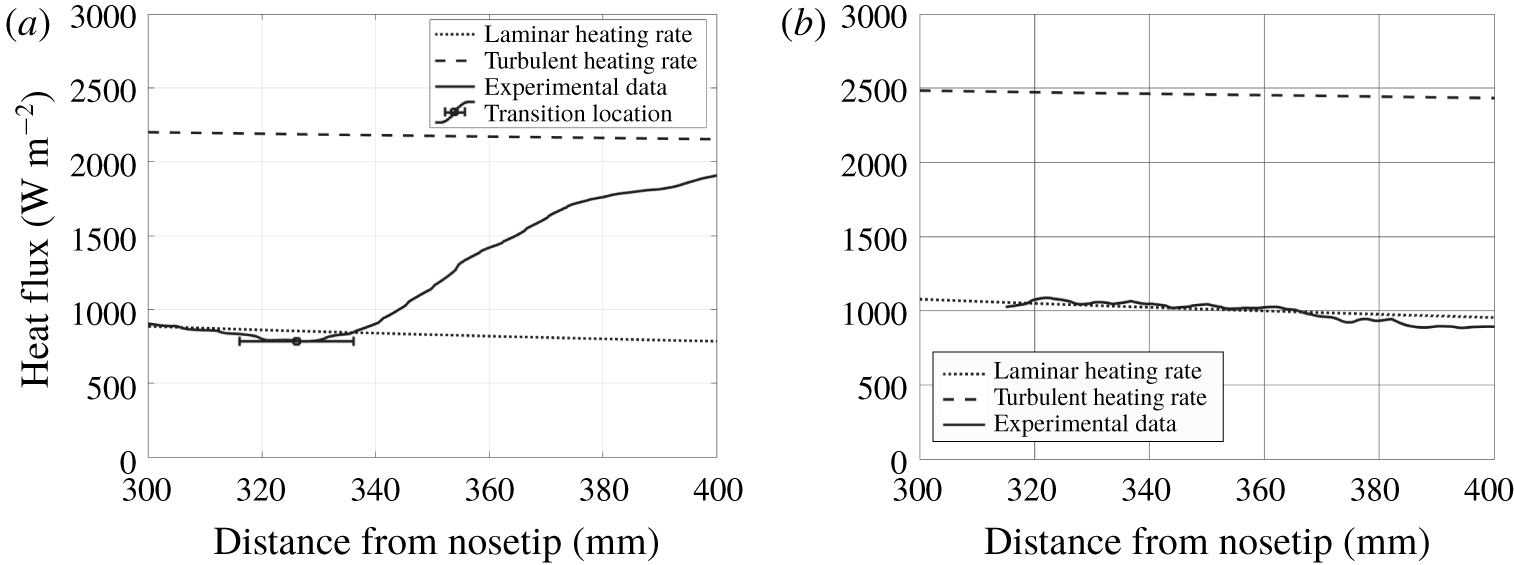
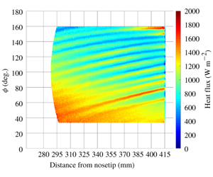
The surface heat-flux data indicated evidence of stationary cross-flow vortices manifested in hot streaks. Two-dimensional heat-flux profiles were extracted from the data along hot streaks and compared with the mean-flow calculations. The data were collected at the same conditions as the computations ( $Re=8.03\times 10^{6}~\text{m}^{-1}$). A heat-flux distribution of the experimental data is given in figure 8. Two paths are given, one along a vortex that exhibited a large heat-flux increase, and one along a vortex that remained near constant values. In figure 9, the corresponding heat-flux profiles from these paths are compared to the fully laminar and fully turbulent heating rates obtained computationally. Figure 9(a) shows the heat flux along vortex path two, which appears to be fully laminar. No significant rise in heat flux was observed for this path. Figure 9(b) shows the heat flux along vortex path one, which appears to be transitional. The laminar region of the data shows good agreement with the computations. A sharp increase in the heating rate on the model was observed at
 $x\approx 340~\text{mm}$. This sharp rise deviated from the expected laminar heating rate, suggesting that transition onset had occurred. The vortex did not appear to become fully turbulent; the heat flux was still increasing at the back edge of the model. The magnitude of the heat flux along this path never reached the expected computational turbulent heating rate.
For the experimental data, a transition location was found by computing linear fits for two portions of the data: one where heat flux was decreasing moving downstream and one where heat flux was increasing downstream, if observed. The intersection point of these fits was concluded to be an estimate of the transition location. Uncertainty estimates were computed by varying the domains of these two regions (Juliano, Paquin & Borg Reference Juliano, Paquin and Borg2019). Based on this technique, the transitional vortex given in figure 9(b) saw a transition location near  $x=340~\text{mm}$ with an uncertainty of
 $\pm 10~\text{mm}$. This location corresponded to where the heat-flux departed from the laminar heating rate in the mean-flow calculations.
The laminar mean-flow results show good agreement with the low heating rates of the experimentally observed hot streaks. The lower heating rates observed between the hot streaks were over-predicted by the laminar mean-flow results. The stationary cross-flow vortices distort the mean flow, making the boundary layer alternately thinner (higher heating rates) and thicker (lower heating rates). The low heating rates between the hot streaks were attributed to this distortion.
Heat-flux distribution.  $\unicode[STIX]{x1D6FC}=6^{\circ }$,
 $Re=8.71\times 10^{6}~\text{m}^{-1}$.

Computational and experimental heat flux along two vortex paths.

4.3 Wavelet analysis
Stationary cross-flow amplification rates are a function of the wavenumber of the vortices. Integrating these amplification rates into an amplitude ratio requires an assumption of which wavenumber to use. Directly extracting these wavenumbers from experimental heat-flux data can improve the stability analysis. Previously, the dominant wavelengths of the heating distribution were calculated with a fast Fourier transform (FFT) analysis of a spanwise heat-flux profile (Schuele, Corke & Matlis Reference Schuele, Corke and Matlis2013; Yates et al. Reference Yates, Juliano, Matlis and Tufts2018). In this application, the usefulness of the FFT is limited because it contained no information regarding the azimuthal variation of the wavelengths.
The wavelet analysis is a mathematical technique well suited for this application. It will be used to determine the wavenumber with the local largest amplitude over the region of interest. By decomposing a time series into time–frequency space, one is able to determine both the dominant modes of variability and how those modes vary in time (Torrence & Compo Reference Torrence and Compo1997). The wavelet transform can be used to analyse time series that contain non-stationary power at many different frequencies (Daubechies Reference Daubechies1990). In this case, azimuthally varying surface heat-flux data were analysed, meaning the analysis was done spatially rather than temporally.
In this work, the continuous wavelet transform (CWT) was used to obtain spatial wavenumber distributions of the stationary cross-flow waves from experimental data. An analytic Morse wavelet was chosen as the mother wavelet because it is effective in analysing modulated signals (Lilly & Olhede Reference Lilly and Olhede2012). The analytic wavelet form was affected by the time–bandwidth product ( $P^{2}$) and the symmetry parameter (
 $\unicode[STIX]{x1D6FE}$), which are non-dimensional parameters defined in the frequency domain. Here,
 $\unicode[STIX]{x1D6FE}=3$, which resulted in a wavelet function with zero skewness. Using a
 $P^{2}$ value of 60 in combination with
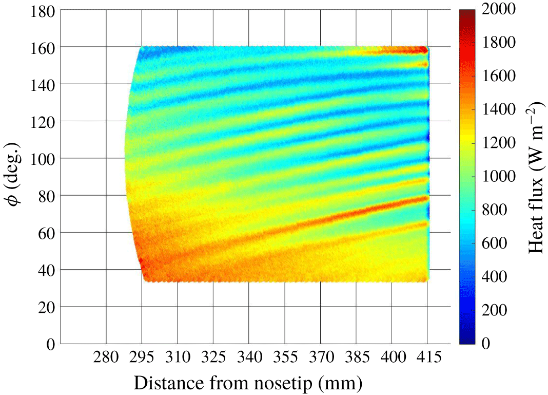
 $\unicode[STIX]{x1D6FE}$ resulted in the desired frequency response. By varying the wavelet scales and translating along the localized index, a picture showing both the amplitude of any features versus the scale and how this amplitude varied spatially was constructed (Torrence & Compo Reference Torrence and Compo1997). Figure 10 shows an example surface heat-flux contour mapped to a
 $x-\unicode[STIX]{x1D719}$ coordinate system. The streaks of high surface heating due to stationary cross-flow vortices are clearly visible in these data. Most of the vortices appear to be fully laminar because they do not see an increase in heating rate expected for a transitional vortex. A vortex at
 $\unicode[STIX]{x1D719}=160^{\circ }$ exhibits higher heating rates far downstream on the model, suggesting that it is transitional.
Heat-flux distribution.  $\unicode[STIX]{x1D6FC}=6^{\circ }$,
 $Re=8.03\times 10^{6}~\text{m}^{-1}$.

The spanwise heat-flux profiles used in the wavelet analysis are finite in length. Because the CWT assumes the data to be cyclic, errors will occur at the beginning and end of the wavelet power spectrum (Torrence & Compo Reference Torrence and Compo1997). The region in which edge effects are important is known as the cone of influence (COI). For this CWT analysis, wavenumber data obtained closest to the windward and leeward rays will fall under the COI. This is not problematic because the transition behaviour on a yawed cone is affected by multiple transition mechanisms and the COI does not cover azimuths where cross-flow is the dominant transition mechanism. Near the leeward symmetry plane under quiet-flow conditions, first and second mode disturbances amplify. This behaviour is similar to supersonic flow in a 2-D boundary layer (Li et al. Reference Li, Choudhari, Chang and White2010). Hot streaks associated with the stationary cross-flow vortices are not expected in this region. Close to the leeward side (at  $\unicode[STIX]{x1D719}\approx 165^{\circ }$), a separation line forms. In this region, the second mode is expected to be the dominant transition mechanism.
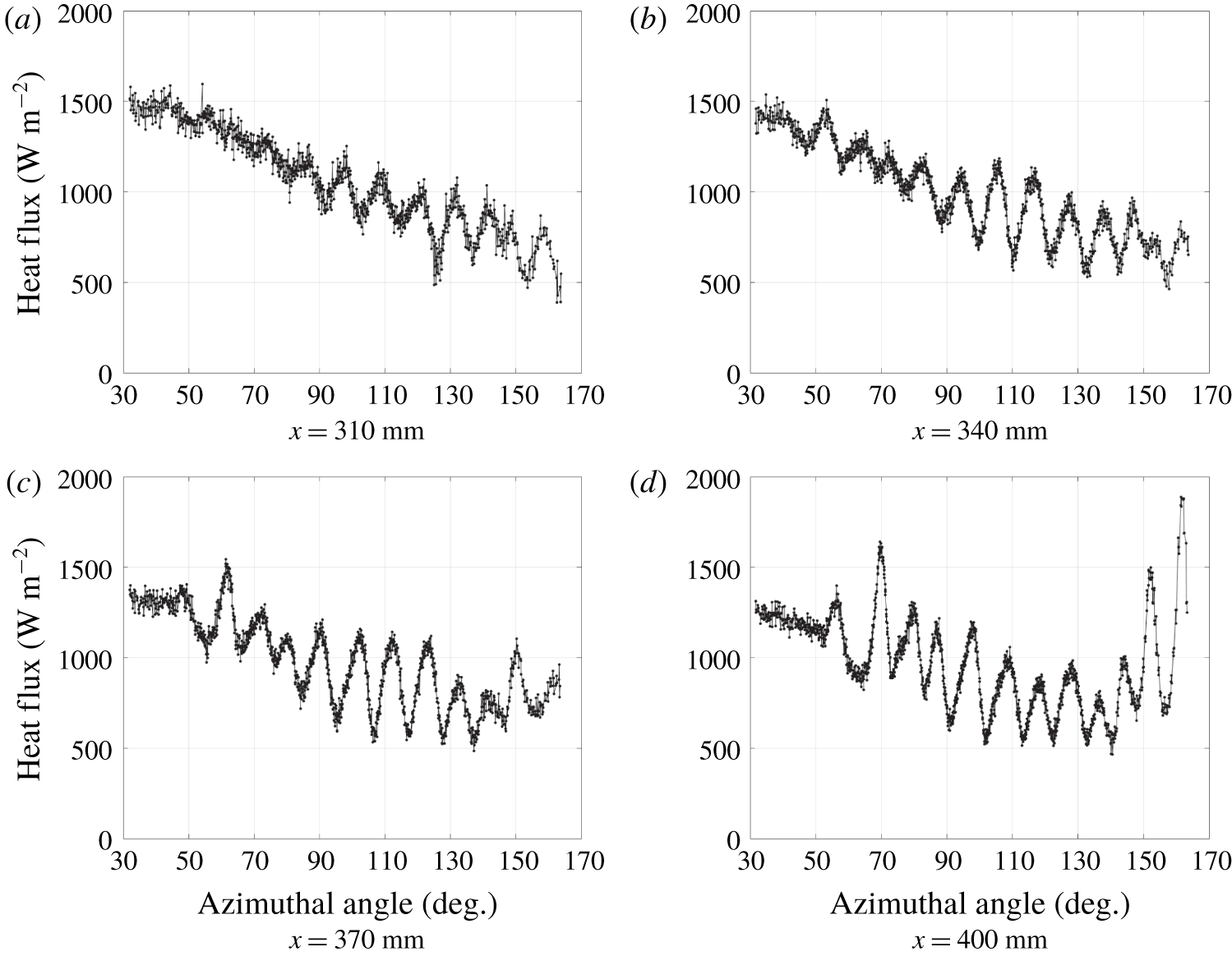
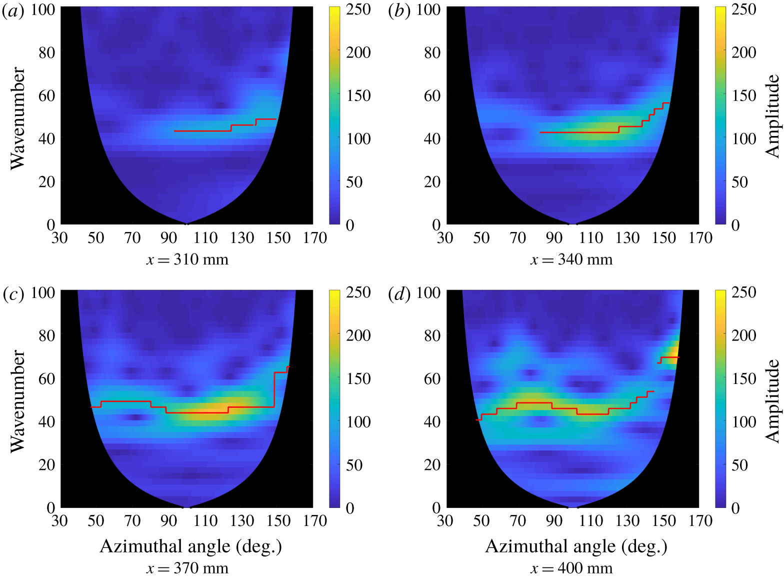
The experimental data were analysed to determine the spatial development of the wavenumber of the naturally occurring largest amplitude stationary waves. To conduct the wavelet analysis, spanwise heat-flux profiles were extracted as a function of azimuth at a constant axial station. Four representative spanwise heat-flux profiles are shown in figure 11. They correspond to the  $x=310$, 340, 370 and 400 mm axial stations of the heat-flux contour shown in figure 10.
Spanwise heat-flux profiles at different axial positions.  $\unicode[STIX]{x1D6FC}=6^{\circ }$,
 $Re=8.03\times 10^{6}~\text{m}^{-1}$.

Each individual spanwise signal was analysed using the CWT technique. The wavelet results corresponding to the representative profiles in figure 11 are given in figure 12. These plots show the local frequency content in terms of the wavenumber at a given spatial position. The contour levels display the amplitude of the heat-flux signal as a function of the wavenumber of the stationary cross-flow waves and azimuth. The resulting wavelength resolution in these data was  $1.80^{\circ }$. The black region on these plots marks the COI from the wavelet analysis. These results show that the peak disturbance amplitudes increase at farther downstream stations. This corresponds to an increase in heat flux along many of the vortices.
Wavelet analysis corresponding to heat-flux profiles in figure 11.

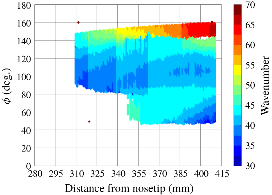
The wavelet analysis was conducted for spanwise heat-flux profiles taken in 1 mm axial increments. This series of CWT amplitudes was used to construct a map of the dominant wavenumber of the stationary cross-flow waves as a function of axial position and azimuth. For the wavelet analysis at a given  $x$, the wavenumber corresponding to the peak amplitude was identified as a function of
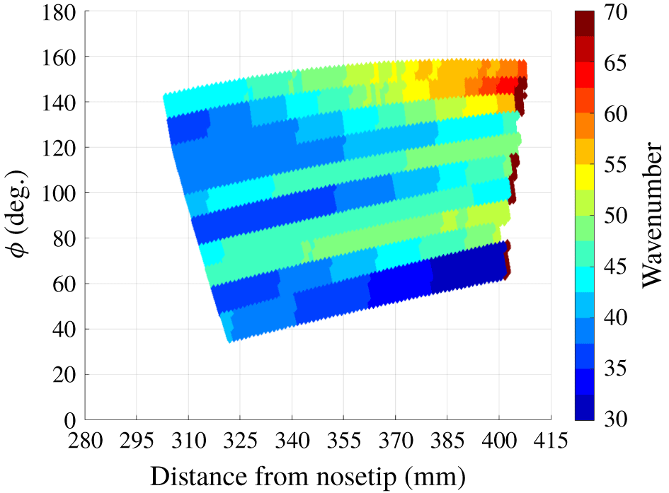
 $\unicode[STIX]{x1D719}$. The red lines in figure 12 trace these peak amplitudes. No peak wavenumber was selected if the maximum amplitude at a given azimuth was below 50. This threshold was set to exclude regions where no hot streaks were observed. Figure 13 shows the results of this analysis for the
 $Re=8.03\times 10^{6}~\text{m}^{-1}$ case (i.e. corresponding to figures 10–12). Figure 13 shows the wavenumber
 $k$ (number of waves per circumference), where
 $k=360^{\circ }/(\unicode[STIX]{x1D706}/R)$ and
 $\unicode[STIX]{x1D706}/R$ is the dominant wavelength normalized by the local radius of curvature of the cone. The contour indicates the spatial distribution of the wavenumber of the stationary cross-flow waves.
Wavenumber of the highest amplitude hot streaks induced by stationary cross-flow vortices.  $Re=8.03\times 10^{6}~\text{m}^{-1}$,
 $\unicode[STIX]{x1D6FC}=6^{\circ }$.

The wavelet analysis revealed a dominant wavenumber between  $k=40$ and
 $k=65$ in the cross-flow region of the cone (between
 $\unicode[STIX]{x1D719}=120^{\circ }$ and
 $160^{\circ }$) for this baseline case. This result agrees well with previous works at similar test conditions. Ward used roughness elements with a critical wavenumber of
 $k=50$ to accelerate transition on a
 $7^{\circ }$ half-angle cone at
 $6^{\circ }$ angle of attack at Mach 6 in the BAM6QT (Ward Reference Ward2014). Li et al. computed a theoretical wavenumber between
 $k=40$ and
 $k=50$ for this configuration corresponding to the most amplified stationary modes under similar free-stream conditions, as seen in the BAM6QT (Li et al. Reference Li, Choudhari, Chang and White2010).
A second technique was pursued to measure the wavenumber of the wavenumber of the hot streaks corresponding to stationary cross-flow waves. This involved directly measuring the distance between the hot streaks. This technique was much more time consuming than the wavelet analysis and offered comparable results. More details are given in the Appendix.
5 Experimental results
Using the CWT analysis, the spatial distribution of the hot streak wavenumbers was calculated for different runs to observe the effect of Reynolds number and angle-of-attack variation on the hot streaks. The experimental results discussed in this paper were all taken on a  $7^{\circ }$ circular cone with a 1.0 mm nose tip diameter and a 101.6 mm base diameter. All wind-tunnel runs were conducted at a free-stream Mach number of 6. The free-stream unit Reynolds number and angle of attack were varied to observe their effect on the wavenumber of the stationary waves. The free-stream unit Reynolds number was varied by conducting individual runs at different total pressures.
5.1 Effect of Reynolds number on wavenumber
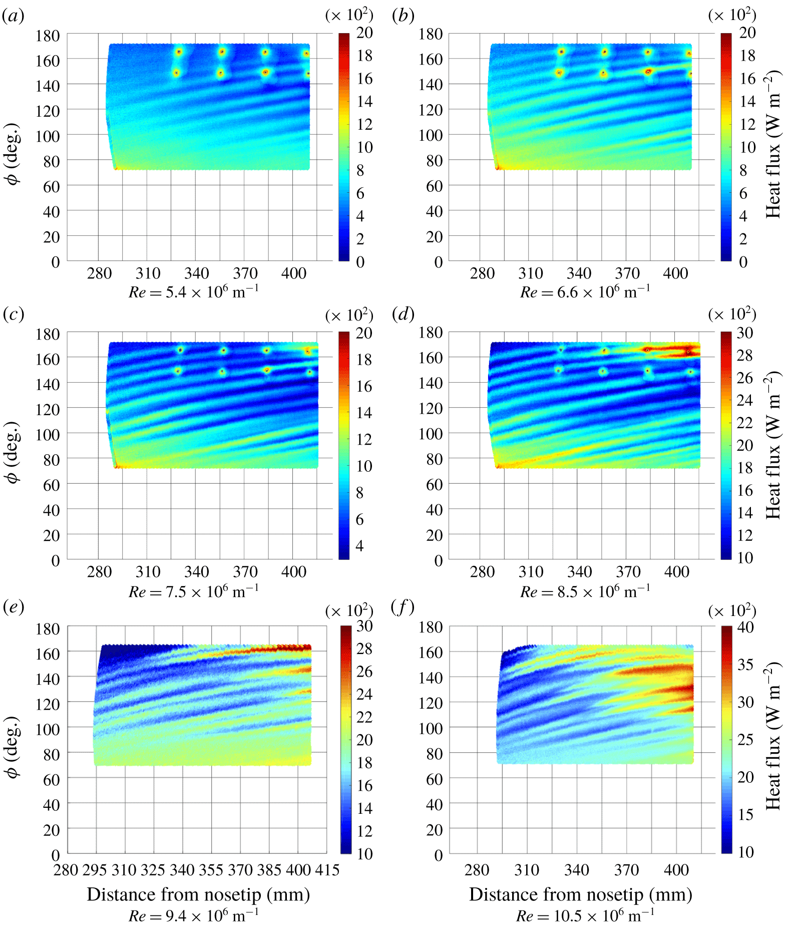
Figure 14 shows IR heat-flux data at six different free-stream unit Reynolds numbers at  $6^{\circ }$ angle of attack. Hot streaks are clearly visible in each image. Heat flux generally increased with increasing Reynolds number. Note that for these data the colour bar scale changes to maximize the visibility of the features. Figure 14(a)–14(d) features eight hot spots between approximately
 $145^{\circ }$ and
 $165^{\circ }$. These correspond to the location of Kulite XCQ-062-15A pressure transducers, which were not used in the current work. Some vortices appear transitional based on the steep increase in heat flux observed along their paths. For the three lowest Reynolds number cases, the streaks maintained their structure, spacing and low levels of heating. This implied that all of the vortices were laminar. At these lower Reynolds numbers, the disturbances are still growing linearly as they progress downstream, but the disturbance amplitudes have not grown large enough to cause transition to occur.
Transitional vortices first appeared near  $\unicode[STIX]{x1D719}=160^{\circ }$ at
 $Re=8.03\times 10^{6}~\text{m}^{-1}$ (figure 14d), but this is in the separated zone close to the leeward plane. Between the separation line and the leeward ray, cross-flow is not the dominant transition mechanism, so these streaks were not necessarily indicative of cross-flow-induced transition. As the Reynolds number was further increased, transitional vortices were observed between
 $\unicode[STIX]{x1D719}=120^{\circ }$ and
 $145^{\circ }$ (figure 14e). At the highest Reynolds number case (figure 14f), ample evidence of cross-flow-induced transition was observed. Streaks between
 $\unicode[STIX]{x1D719}=110^{\circ }$ and
 $150^{\circ }$ exhibited large increases in heat flux and they began to spread azimuthally. At higher Reynolds numbers, the higher heating rates along the hot streaks indicated that the disturbance amplitudes had grown large enough to cause transition to occur.
Above  $Re=8.5\times 10^{6}~\text{m}^{-1}$, some hot streaks appeared to weaken, but give rise to adjacent streaks that became turbulent. Edelman observed similar structures on a cone at angle of attack at conditions similar to those of the current work (Edelman Reference Edelman2019). He referred to them as ‘wishbone structures’, and suggested they may be due to a pair of co-rotating vortices. We suspect that the upstream streaks are due to the mean-flow distortion of the stationary cross-flow waves, whereas the nascent streaks arise from the secondary instability that are the proximate cause of transition. The surface heating footprints of the secondary instabilities are anchored to the primary instabilities, but not directly in line with them.
Effect of free-stream unit Reynolds number on surface heat flux.  $\unicode[STIX]{x1D6FC}=6^{\circ }$.

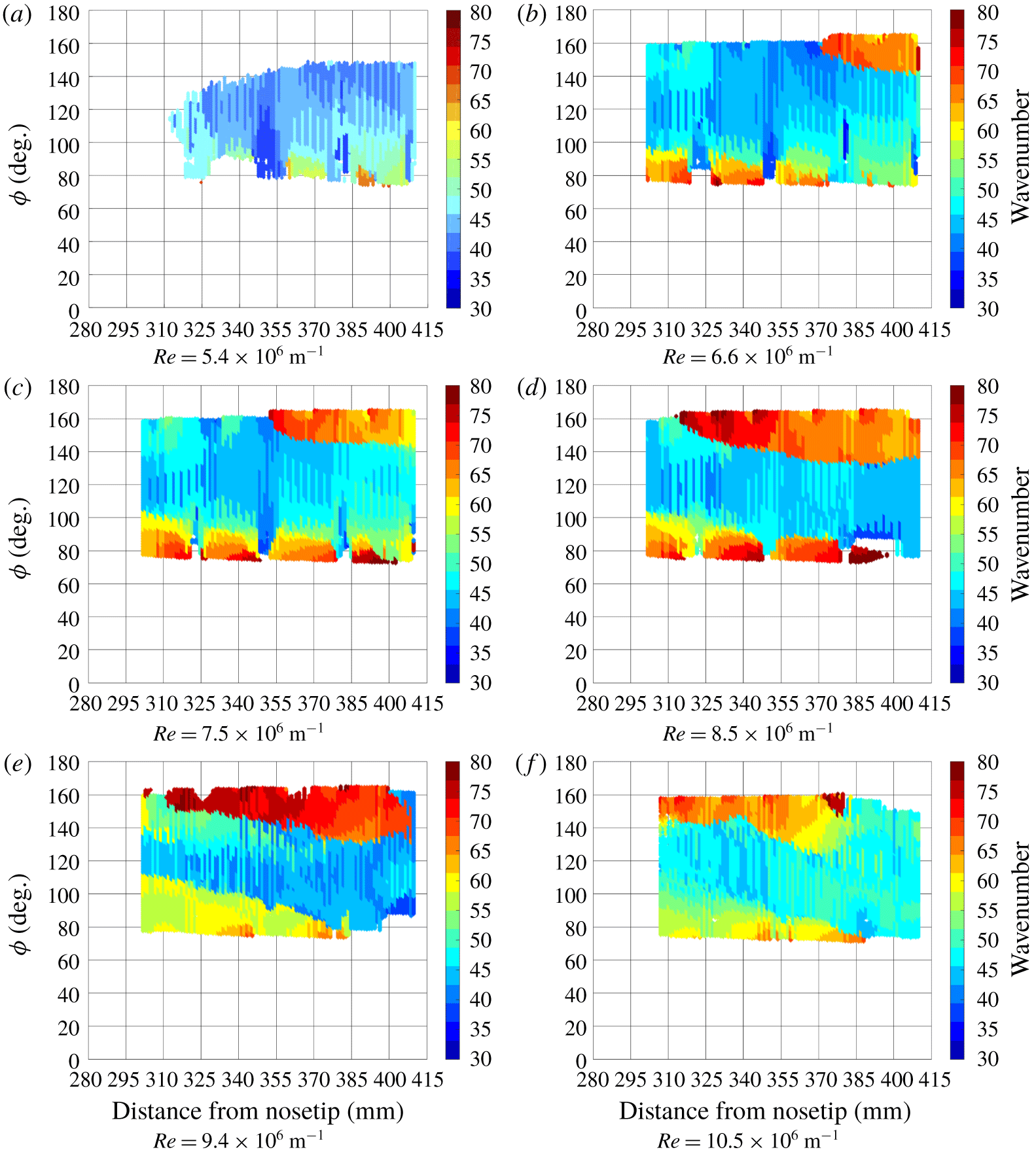
Effect of free-stream unit Reynolds number on wavenumber.  $\unicode[STIX]{x1D6FC}=6^{\circ }$.

The wavelet analysis was applied to these six test cases using spanwise heat-flux profiles as the input. The results, showing the local wavenumber distribution of the experimentally observed hot streaks, are given in figure 15. The observed hot streaks, which correspond to the stationary cross-flow waves, became more distinct with increasing Reynolds number. This is reflected in the wavelet analysis, where amplitudes above the cutoff threshold were observed over a larger portion of the surface as the Reynolds number increased. For most cases, the wavenumber increased towards the leeward ray. The boundary layer is known to thicken near the leeward ray for this configuration, resulting in a distinct, mushroom-like structure (Li et al. Reference Li, Choudhari, Chang and White2010). The observed increase in the wavenumber near the leeward ray is related to the separation line that forms due to this phenomenon.
Between  $\unicode[STIX]{x1D719}=100^{\circ }$ and
 $140^{\circ }$, local wavenumbers between
 $k=40$ and 55 were observed. In this azimuthal range of the model, cross-flow is the dominant transition mechanism. In this region, the wavenumbers were fairly uniform spatially and did not vary strongly as a function of Reynolds number. Closer to windward (
 $\unicode[STIX]{x1D719}\lesssim 100^{\circ }$), the wavenumbers are higher than in the zone of peak cross-flow, and no distinct streaks were observed for
 $\unicode[STIX]{x1D719}\lesssim 75^{\circ }$. Li computed amplification factors for stationary cross-flow vortex instabilities for the same geometry and similar test conditions (Li et al. Reference Li, Choudhari, Chang and White2010). N-factors of 10 or higher were concluded to correspond to cross-flow-induced transition. This was seen down to an angle of
 $\unicode[STIX]{x1D719}=80^{\circ }$ at
 $x=300~\text{mm}$ and
 $\unicode[STIX]{x1D719}=60^{\circ }$ at
 $x=400~\text{mm}$ in the computations (Li et al. Reference Li, Choudhari, Chang and White2010). Therefore, the observed increase in wavenumber in figure 15 was still in the azimuthal range where cross-flow-induced transition could be expected.
To demonstrate the repeatability of the data, multiple runs were conducted at nominally identical unit Reynolds numbers. The model configuration, including the nose tip orientation, was held constant for these tests. Resulting heat-flux distributions showed that the hot streaks’ behaviour was similar between runs. The streaks formed at the same azimuths and exhibited similar heating rates. The resulting wavenumber distributions were repeatable and showed good agreement between runs. This consistency suggests that the stationary cross-flow vortices were anchored to model roughness, rather than being a stochastic function of the tunnel’s startup process and establishment of the flow field.
Effect of  $\unicode[STIX]{x1D6FC}$ and
 $Re$ on surface heat flux.

5.2 Effect of angle of attack on wavenumber
Runs were conducted to investigate the effect of angle of attack on the local wavenumber of the stationary cross-flow waves. Data were collected for two unit Reynolds numbers at  $4^{\circ }$ and
 $6^{\circ }$ angle of attack. At a lower angle of attack, the circumferential pressure gradient is weakened. This in turn reduces the magnitude of the cross-flow velocity component in the boundary layer.
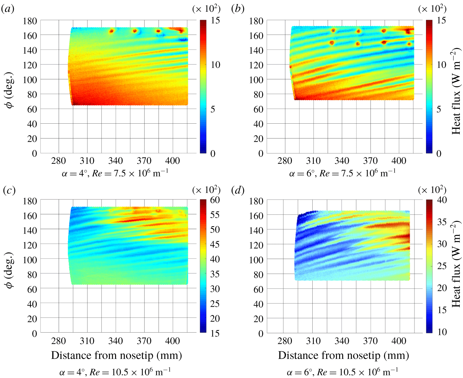
Figure 16 shows angle-of-attack variation at two unit Reynolds numbers. Note that the colour bar scale varies among the panels to improve the visibility of the flow features. Again, dots corresponding to the Kulite pressure transducers are visible in some of the images. Figures 16(a) and 16(b) show two runs at  $Re=7.9\times 10^{6}~\text{m}^{-1}$ at
 $4^{\circ }$ and
 $6^{\circ }$ angle of attack. Clear, distinct hot streaks were observed for each run, but they did not appear to transition at the lower Reynolds number. At a
 $4^{\circ }$ angle of attack, the hot streaks were most distinct between
 $\unicode[STIX]{x1D719}=100^{\circ }$ and
 $160^{\circ }$. In contrast to the
 $6^{\circ }$ angle of attack case, vortices were generally not observed between the windward ray and
 $\unicode[STIX]{x1D719}=100^{\circ }$. This indicated the azimuthal range of cross-flow-induced transition expanded to include lower azimuths as angle of attack increased. Figures 16(c) and 16(d) show angle-of-attack variation at
 $Re=11.1\times 10^{6}~\text{m}^{-1}$. Transitional vortices, characterized by rapid increases in heat flux, were observed for both angles of attack. At a
 $4^{\circ }$ angle of attack, rapid heat-flux increases were observed between
 $\unicode[STIX]{x1D719}=120^{\circ }$ and the leeward ray. These streaks reached higher heat-flux compared to the
 $6^{\circ }$ angle of attack run. On the windward side of a cone, heat flux increases for increasing angle of attack, but the opposite trend is true on the leeward side. The fluid from the boundary-layer edge pushed closer to the wall by the vortices at higher azimuth was processed by a stronger shock at lower angle of attack, hence the higher heat flux.
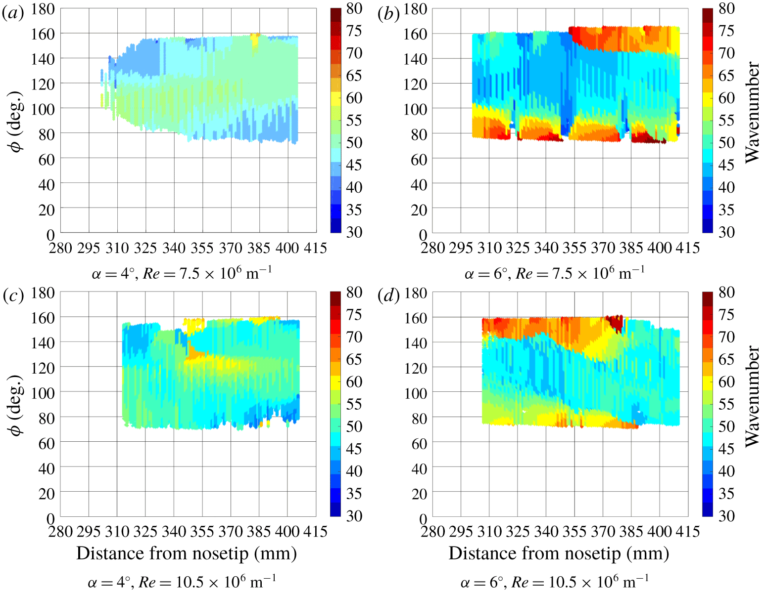
The data from figure 16 were analysed using the wavelet analysis technique with spanwise heat-flux profiles (figure 17). The same amplitude threshold of 50 was applied. For both free-stream unit Reynolds numbers, similar wavenumbers were generally observed at each angle of attack between  $\unicode[STIX]{x1D719}=100^{\circ }$ and
 $145^{\circ }$. The wavenumbers were more uniform at
 $4^{\circ }$ angle of attack compared to the
 $6^{\circ }$ cases. This was attributed to the weaker spanwise pressure gradient at
 $4^{\circ }$ angle of attack compared to
 $6^{\circ }$ angle of attack.
Effect of  $\unicode[STIX]{x1D6FC}$ and
 $Re$ on wavenumber.

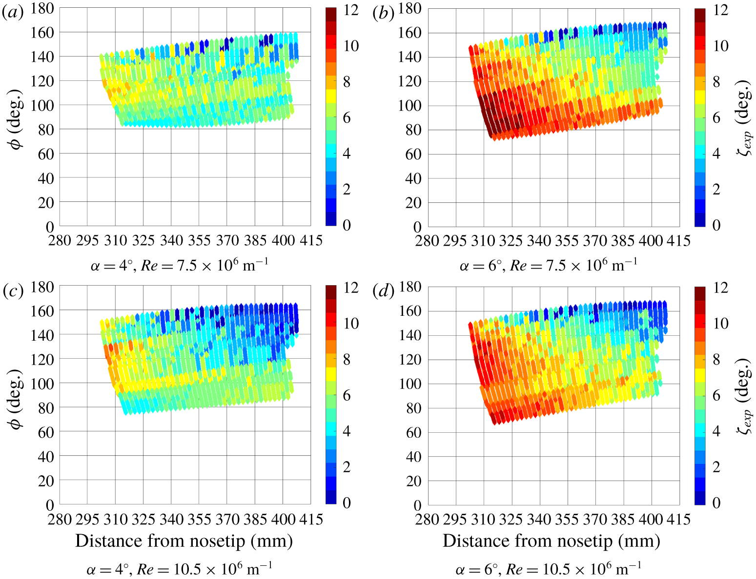
To further investigate the hot-streak behaviour with angle-of-attack variation, the relative angles between the streaks and the local line of constant azimuth,  $\unicode[STIX]{x1D701}_{exp}$, were computed. Figure 18 gives the resulting hot-streak angles for each run. At each unit Reynolds number, the angle of attack had a large effect on the hot-streak angles. Figures 18(a) and 18(b) show hot-streak angles at
 $4^{\circ }$ and
 $6^{\circ }$ angle of attack at
 $Re=7.5\times 10^{6}~\text{m}^{-1}$. Both runs show the highest hot-streak angles occurred at the furthest upstream locations. The hot-streak angles decreased downstream and near the leeward ray; the angles reached low values as the hot streaks approached the separation line. Near the separation line, the angle of attack did not affect the hot-streak angles. The largest effect of angle of attack on the hot-streak angles occurred near the upstream portion of the images towards the windward ray. All these observations are explained by the effect of the angle of attack on the circumferential pressure gradient: a stronger pressure gradient causes greater inclination of the vortex paths. Substantial spatial variation is visible when surveying the global heat-flux contour – simply reporting a mean or representative streak angle would not characterize the flow field well.
Effect of  $\unicode[STIX]{x1D6FC}$ and
 $Re$ on relative streak angle.

6 Stability analysis with experimentally observed wavenumbers
The results of the wavelet analysis and previous studies show that, over the surface of a yawed cone, the stationary cross-flow vortices are not uniformly spaced azimuthally around the cone’s surface (Perez, Reed & Kuehl Reference Perez, Reed and Kuehl2013; Schuele et al. Reference Schuele, Corke and Matlis2013; Moyes et al. Reference Moyes, Kocian, Mullen and Reed2017; Yates et al. Reference Yates, Juliano, Matlis and Tufts2018, Reference Yates, Juliano, Matlis and Tufts2019). Vortices tend to emanate near the attachment line on the windward ray of the cone and become unequally distributed moving towards the leeward ray. The unequal distribution of the vortices results in variation of the local wavenumber over the surface of the cone. Because the local amplification rate is a function of wavenumber, properly modelling the spatial wavenumber variation of the vortices is a critical step in integrating those amplification rates to accurate N-factors. In this work, three different models for the spatial wavenumber variation were employed and compared: the computed locally most amplified wavenumber of the stationary waves, a hybrid technique using computed vortex spreading (Moyes et al. Reference Moyes, Kocian, Mullen and Reed2017) anchored by experimentally observed wavenumbers, or the experimentally observed largest amplitude wavenumbers.
6.1 Computational methods
The LASTRAC3d (Chang Reference Chang2003, Reference Chang2004a,Reference Changb) stability suite was used to solve the LST/PSE stability equations. An in-house Fortran script converted the Overflow2.2n formatted solution to a LASTRAC3d formatted mean-flow file without interpolation. The solution was projected to the wall-normal direction while calculating the wall-normal distance in accordance with the LASTRAC3d manual (Chang Reference Chang2004b). LASTRAC3d was used to calculate the spatial growth rates of the stationary cross-flow instabilities for a range of wavenumbers. The wavenumber was defined as the number of waves that would be present on the surface of the cone if the local wavelength was constant about the cones circumference. This spacing was measured orthogonal to the cones axis, not the flows.
6.1.1 Linear stability theory
To solve for the stability characteristics, we define a solution vector  $\boldsymbol{Q}$ containing the primitive variables:
 $$\begin{eqnarray}\boldsymbol{Q}=[u,v,w,\unicode[STIX]{x1D70C},T]^{\intercal }.\end{eqnarray}$$
One may then write the full nonlinear Navier–Stokes equations as an operator  ${\mathcal{N}}$ which gives the general form of the equations:
 $$\begin{eqnarray}\frac{\unicode[STIX]{x2202}\boldsymbol{Q}}{\unicode[STIX]{x2202}t}={\mathcal{N}}\boldsymbol{Q}.\end{eqnarray}$$
By writing the equations in this form, we can perform derivations without the loss of generality. If we then decompose the solution vector  $\boldsymbol{Q}$ into a non-time dependent base state
 $\overline{\boldsymbol{Q}}$ and a time-varying perturbation
 $\boldsymbol{q}^{\prime }$ assumed to be of small magnitude
 $O(\unicode[STIX]{x1D700})$ such that
 $$\begin{eqnarray}\boldsymbol{Q}=\overline{\boldsymbol{Q}}+\boldsymbol{q}^{\prime },\end{eqnarray}$$
and separate the linear  $O(\unicode[STIX]{x1D700})$ terms from the nonlinear
 $O(\unicode[STIX]{x1D700}^{2})$ terms, we can define the linear Navier–Stokes equations (LNSE). These can be written as an initial value problem in terms of operators:
 $$\begin{eqnarray}{\mathcal{B}}\frac{\unicode[STIX]{x2202}\boldsymbol{q}^{\prime }}{\unicode[STIX]{x2202}t}={\mathcal{A}}\boldsymbol{q}^{\prime }+O(\unicode[STIX]{x1D700}^{2}).\end{eqnarray}$$
Depending on the desired application, these equations may also be written separating out spatial derivatives in a nonlinear form:
 $$\begin{eqnarray}{\mathcal{B}}_{1}\frac{\unicode[STIX]{x2202}\boldsymbol{q}^{\prime }}{\unicode[STIX]{x2202}x}+{\mathcal{B}}_{2}\frac{\unicode[STIX]{x2202}^{2}\boldsymbol{q}^{\prime }}{\unicode[STIX]{x2202}x^{2}}={\mathcal{A}}\boldsymbol{q}^{\prime }+O(\unicode[STIX]{x1D700}^{2}).\end{eqnarray}$$
Starting from (6.4), we can define our assumptions about  $\overline{\boldsymbol{q}}$ and the form of
 $\boldsymbol{q}^{\prime }$. For LST, we define
 $\overline{\boldsymbol{q}}=\overline{\boldsymbol{q}}(y)$, meaning the base flow solution varies only in the wall-normal direction, and is homogeneous in the other two directions. This lends itself to the form of disturbances given by the assumption of normal modes. The disturbances should be discretized in the same dimensions as the underlying basic state, and represented in Fourier space in the homogeneous directions as well as in time. For example, using the form for one inhomogeneous direction results in the set of equations typically called the linear stability theory equations,
 $$\begin{eqnarray}\boldsymbol{q}^{\prime }=\hat{\boldsymbol{q}}(\,\boldsymbol{y})\text{e}^{\text{i}(\unicode[STIX]{x1D6FC}x+\unicode[STIX]{x1D6FD}z-\unicode[STIX]{x1D714}t)}+\text{c.c.}\end{eqnarray}$$
In general,  $\unicode[STIX]{x1D6FC}$,
 $\unicode[STIX]{x1D6FD}$ and
 $\unicode[STIX]{x1D714}$ are all complex and c.c. is the complex conjugate of the first term on the right-hand side (Kuehl Reference Kuehl2016). Using this mode is equivalent to a Fourier transform in time and a Laplace transform in space. Substitution of this ansatz into (6.4) (along with removing the base state solution, which is identically zero, and discarding the
 $O(\unicode[STIX]{x1D700}^{2})$ or higher terms) allows for the creation of a generalized, linear, temporal eigenvalue problem of the form
 $$\begin{eqnarray}(\unicode[STIX]{x1D714}B-A)\hat{\boldsymbol{q}}=0.\end{eqnarray}$$
In this formulation,  $\unicode[STIX]{x1D6FC}$ and
 $\unicode[STIX]{x1D6FD}$ are taken to be real parameters, and
 $\unicode[STIX]{x1D714}$ is complex and part of the solution. To derive the LST equations, an assumption was made that one or more directions were spatially discretized, and the remaining dimensions were locally homogeneous. However, given the derivation of the LNSE separation of scales, it is possible to consider a ‘slowly varying’ direction such that the spatial gradients are not
 $O(1)$ but rather
 $O(\unicode[STIX]{x1D700})$. This slowly varying direction is typically taken to be the streamwise direction. However, the spatial problem is of more interest than the temporal problem. Examining the LNSE operator as written in (6.5) reveals that the equations are nonlinear in terms of spatial derivatives, resulting in a quadratic eigenvalue problem of the form
 $$\begin{eqnarray}(\unicode[STIX]{x1D6FC}B_{1}+\unicode[STIX]{x1D6FC}^{2}B_{2}-A)\hat{\boldsymbol{q}}=0.\end{eqnarray}$$
This is then converted to a linear eigenvalue problem using the companion matrix method, wherein  $\hat{\boldsymbol{q}}$ is redefined as
 $\hat{\boldsymbol{q}}^{+}$ containing the first of the quadratic terms. For example, if
 $\hat{\boldsymbol{q}}=[u,\,v,\,w,\,p]^{\intercal }$, then
 $\hat{\boldsymbol{q}}^{+}=[u,\,v,\,w,\,p,\,\unicode[STIX]{x1D6FC}u,\,\unicode[STIX]{x1D6FC}v,\,\unicode[STIX]{x1D6FC}w,\,\unicode[STIX]{x1D6FC}p]^{\intercal }$. Doing so results in an eigenvalue problem of the form
 $$\begin{eqnarray}(\unicode[STIX]{x1D6FC}B-A)\hat{\boldsymbol{q}}^{+}=0.\end{eqnarray}$$
In this formulation,  $\unicode[STIX]{x1D714}$ and
 $\unicode[STIX]{x1D6FD}$ are taken to be real parameters, and
 $\unicode[STIX]{x1D6FC}$ is complex and part of the solution. Equation (6.9) is the form solved in LASTRAC for the current work’s LST results, where the operators
 $A$ and
 $B$ are given by the compressible form of the Navier–Stokes equations. For further details on LASTRAC’s specific implementation see Chang (Reference Chang2003) and Chang (Reference Chang2004b).
6.1.2 Linear parabolized stability equations
To derive the parabolized stability equations, one replaces the normal mode ansatz using constant wavenumber parameters (e.g. (6.6)) with an ansatz that contains a phase function that will allow for both ‘slow’ changes in the basic state and ‘slow’ changes in the shape of the disturbance in one or more directions. In this formulation, both the wave function  $\unicode[STIX]{x1D6FC}(x)$ and the shape function
 $\hat{\boldsymbol{q}}$ are considered to vary with the
 $x$ direction. These variations are defined as ‘slow’ with
 $x$, such that their derivatives are
 $O(\unicode[STIX]{x1D700})$. This distinction is denoted by replacing
 $x$ with the dummy variable
 $\unicode[STIX]{x1D713}$:
 $$\begin{eqnarray}\boldsymbol{q}^{\prime }=\hat{\boldsymbol{q}}(x,y)\;\text{e}^{(\text{i}\int _{x}\unicode[STIX]{x1D6FC}(\unicode[STIX]{x1D713})\,\text{d}\unicode[STIX]{x1D713})}\;\text{e}^{\text{i}(\unicode[STIX]{x1D6FD}z-\unicode[STIX]{x1D714}t)}+\text{c.c.}\end{eqnarray}$$
After substituting in (6.10), the equations given by (6.4) then take on a form given by
 $$\begin{eqnarray}L\hat{\boldsymbol{q}}+M\frac{\unicode[STIX]{x2202}\hat{\boldsymbol{q}}}{\unicode[STIX]{x2202}x}=F.\end{eqnarray}$$
Because the term  $\unicode[STIX]{x2202}\hat{\boldsymbol{q}}/\unicode[STIX]{x2202}x$ is now non-zero, this form is no longer separable into an eigenvalue problem (even in the linear form where
 $F=0$). In practice, this is solved as an initial value problem using the spatial direction as a pseudo-time step. The initial condition is typically an unstable eigenmode derived from LST. Further detail on the implementation in LASTRAC is found in Chang (Reference Chang2003) and Chang (Reference Chang2004b).
6.1.3 Solving for group velocity
In general, the group velocity direction is the propagation direction of a wave packet. Mathematically this direction is found by finding the dispersion relation between individual wave components, found by solving for the real part of the quantity
 $$\begin{eqnarray}\left.\frac{\text{d}\unicode[STIX]{x1D714}}{\text{d}\unicode[STIX]{x1D6FD}}\right/\frac{\text{d}\unicode[STIX]{x1D714}}{\text{d}\unicode[STIX]{x1D6FC}}=\frac{\text{d}\unicode[STIX]{x1D6FC}}{\text{d}\unicode[STIX]{x1D6FD}}.\end{eqnarray}$$
In this case,  $\unicode[STIX]{x1D714}$ represents the temporal wavenumber, while the spatial wavenumber is given by
 $\unicode[STIX]{x1D6FC}$ and
 $\unicode[STIX]{x1D6FD}$ in the streamwise and spanwise directions, respectively. Within the framework of LASTRAC, this is found by first allowing
 $\unicode[STIX]{x1D6FD}$ to be real (consistent with the assumptions given by LST). Then complex
 $\unicode[STIX]{x1D6FC}$ is solved for by finding the solution with
 $\text{d}\unicode[STIX]{x1D6FC}_{I}/\text{d}\unicode[STIX]{x1D6FD}=0$. The corresponding group velocity direction is then given by
 $\text{d}\unicode[STIX]{x1D6FC}_{R}/\text{d}\unicode[STIX]{x1D6FD}$. Further detail is found in Chang (Reference Chang2004b). The LASTRAC3d study output the group velocity pathline of the stationary waves with an optimal spatial growth rate. For stationary cross-flow waves, this is the direction such that the cross-flow velocity profile has its inflection point at zero velocity.
6.2 Comparison of computational marching directions with experimental data
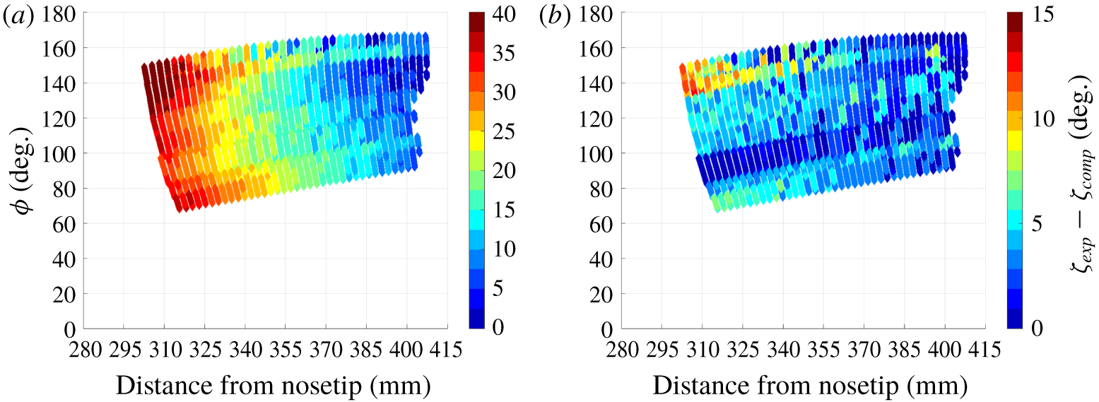
The group velocity pathline marching direction was predicted to correspond with the stationary cross-flow vortex paths. Additionally, inviscid streamline paths were computed for each test case. Figure 19 examines which computationally generated trajectory – inviscid streamlines or group velocity pathlines – more accurately models the trajectories of the hot streaks observed in the experiments. The experimentally observed hot streaks are presumed to arise from the stationary cross-flow vortices. The comparison was done by first measuring the angle of the inviscid streamlines, group velocity pathlines and experimentally observed hot-streak pathlines relative to the cone axis. The relative angle between the experimental and computational data ( $\unicode[STIX]{x1D701}_{exp}-\unicode[STIX]{x1D701}_{comp}$) was computed by finding the difference between these two angles.
The computed relative angles between the computationally derived inviscid streamlines (figure 19a) and experimentally observed hot streaks are relatively large,  ${\approx}30^{\circ }$ at
 $x=300~\text{mm}$ decreasing to
 ${\approx}10^{\circ }$ by the end of the model. This shows that the inviscid streamlines do not correspond well with the trajectories of the hot streaks observed in the experiment. In contrast, the computed relative angles between the group velocity pathlines and experimentally observed hot streaks are small (
 ${\approx}5^{\circ }$ or less) at nearly every observed location on the model (figure 19b). That is, the computed group velocity pathlines agree well with the trajectories of the experimentally observed hot streaks. For this reason, stability analyses of stationary cross-flow vortices should use group velocity pathlines as the marching direction. N-factors for this study were integrated along the group velocity paths in all cases.
Difference between computationally derived marching directions with observed hot-streak trajectories.  $\unicode[STIX]{x1D6FC}=6^{\circ }$,
 $Re=10.5\times 10^{6}~\text{m}^{-1}$.

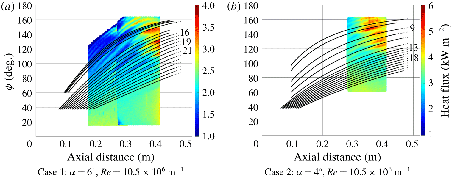
Figure 20 overlays the group velocity pathlines for two cases with the experimental heat-flux contours. Case 1, given in figure 20(a), shows experimental data from two different wind-tunnel runs at the same free-stream unit Reynolds number and angle of attack. Conducting two separate runs was desirable to image further upstream on the model, as optical access was limited by the IR window. The computed group velocity pathlines for this case showed very good agreement with the hot streaks observed in the experiment. The group velocity pathlines and hot streaks emanated near the windward ray and curved towards the leeward ray moving downstream. Case 2 is given in figure 20(b). Again, very good agreement was demonstrated between the computed group velocity pathlines and hot streaks. Figure 20 also shows labels for the group velocity pathlines. Wavenumber variation, and subsequently N-factors, were computed along these pathlines.
Comparison of the computed group velocity pathlines and experimental heat-flux data.

For each integration path, the spatial growth rate output from LASTRAC3d was used to create a piecewise cubic-spline interpolating function across the surface of the cone. The function returned the spatial growth rate as a function of axial distance  $x$, the azimuthal angle
 $\unicode[STIX]{x1D719}$, and the local wavenumber
 $k$. This made it possible to integrate an N-factor using an arbitrarily varying wavenumber along a given pathline.
6.3 N-factor results
The N-factor is the spatial amplification rate of a disturbance integrated along its path. The amplification rate is a function of the local wavenumber of the stationary cross-flow waves and many other variables. The local wavenumber was determined using three techniques and the resulting N-factors are compared for each. For the first technique, the locally most unstable (highest amplification rate) wavenumbers were used at every step along the integration path. This method yields the maximum possible stationary cross-flow vortex amplitude for a given pathline. Because of its conservative nature, this is the conventional method used to calculate N-factors in three-dimensional flow fields.
The second technique determined the local spreading of neighbouring vortices based on the computed vortex pathlines (Moyes et al. Reference Moyes, Kocian, Mullen and Reed2017). In this approach, the basic state is adjusted to model the evolution of the wavenumber in the direction perpendicular to the marching path. In the current work, the marching path is along group velocity pathlines. The technique assumes a physical number of spanwise waves remain constant between neighbouring vortex paths. As the paths progress downstream, the azimuthal spacing between them may increase or decrease. This change, along with the local orientation of the disturbance path, is used to measure the normal distance between paths. This gives values for the local effective wavenumber.
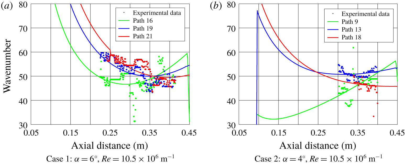
Using this technique, a non-dimensional ratio of the local wavenumber along each group velocity pathline was computed. The wavenumber ratio was defined as the local wavenumber divided by the wavenumber defined at the first available data point along the integration paths. Because the wavenumber ratios defined a relative rather than absolute wavenumber, this technique required dimensionalizing the computed values, which was done with experimental data. Along a given integration path, a single reference wavenumber at one axial position was used to normalize the wavenumber ratio. This axial station was selected separately for each path in order to yield the best fit between the experimental wavenumbers and the dimensionalized computational wavenumbers in the least-squares sense. The wavenumber used to compute the amplification rate at each location is thus a hybrid of the computed and experimental data.
The best-fit wavenumber distribution is plotted with the experimentally measured values for three representative pathlines in figure 21. Figure 21(a) shows wavenumber data along three paths: 16, 19 and 21. The labels of these paths correspond to labelled pathlines in figure 20(a). At  $x=0.4~\text{m}$, these paths are all located between
 $\unicode[STIX]{x1D719}=100^{\circ }$ and
 $140^{\circ }$. Path 16 is located closest to the leeward ray; higher path numbers correspond to pathlines located closer to the windward ray. Likewise, the paths in figure 21(b) correspond to the labelled pathlines in figure 20(b). They are located in a similar azimuthal range at
 $x=0.4~\text{m}$ and follow the same naming convention.
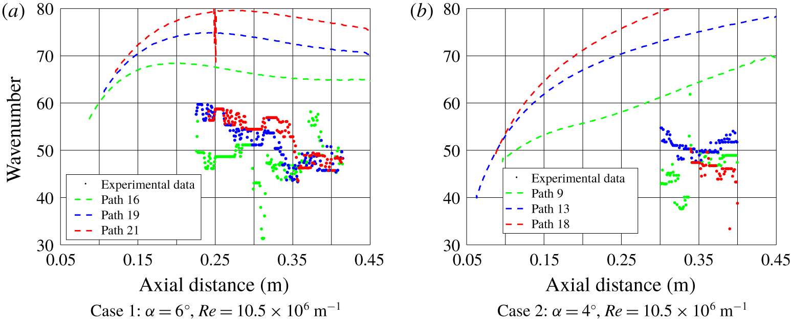
The best-fit computed wavenumber profiles fit the experimental results well for both cases – the trends are accurately captured and the computed profiles exhibit much less scatter than the experimental data. Most importantly, they permit extrapolation upstream, to where the vortex amplitudes are too low to affect surface heating sufficiently to be discerned by IR thermography. In contrast, the locally most unstable wavenumbers do not correspond well with the experimentally observed wavenumbers of largest amplitude (figure 22). The LST computations from this technique yield the most unstable wavenumbers, i.e. the ones with the largest amplification rate. This method relies only on computed amplification rates. The experimental measurements, on the other hand, are of the wavenumbers with the largest local amplitudes. These two properties are closely related, but they are not identical, so the lack of correspondence between the experimental data and most unstable wavenumbers was expected. Figure 22 shows that the most unstable wavenumbers were much higher than the largest amplitude wavenumbers for each case.
The third technique to compute N-factors uses the amplification rate calculated for cross-flow waves with wavenumbers equal to the experimentally observed largest amplitude hot streaks along each integration path. Computed vortex path spreading is not used. Because this method is agnostic of the wavenumber upstream of the IR cameras field of view, the N-factor at that station ( $x=295~\text{mm}$) was assumed to equal the N-factor for the hybrid computational/experimental method.
Comparison of the computationally varying azimuthal wavenumber with the experimental largest amplitude wavenumber.

Comparison of the computationally most unstable wavenumber with the experimental largest amplitude wavenumber.

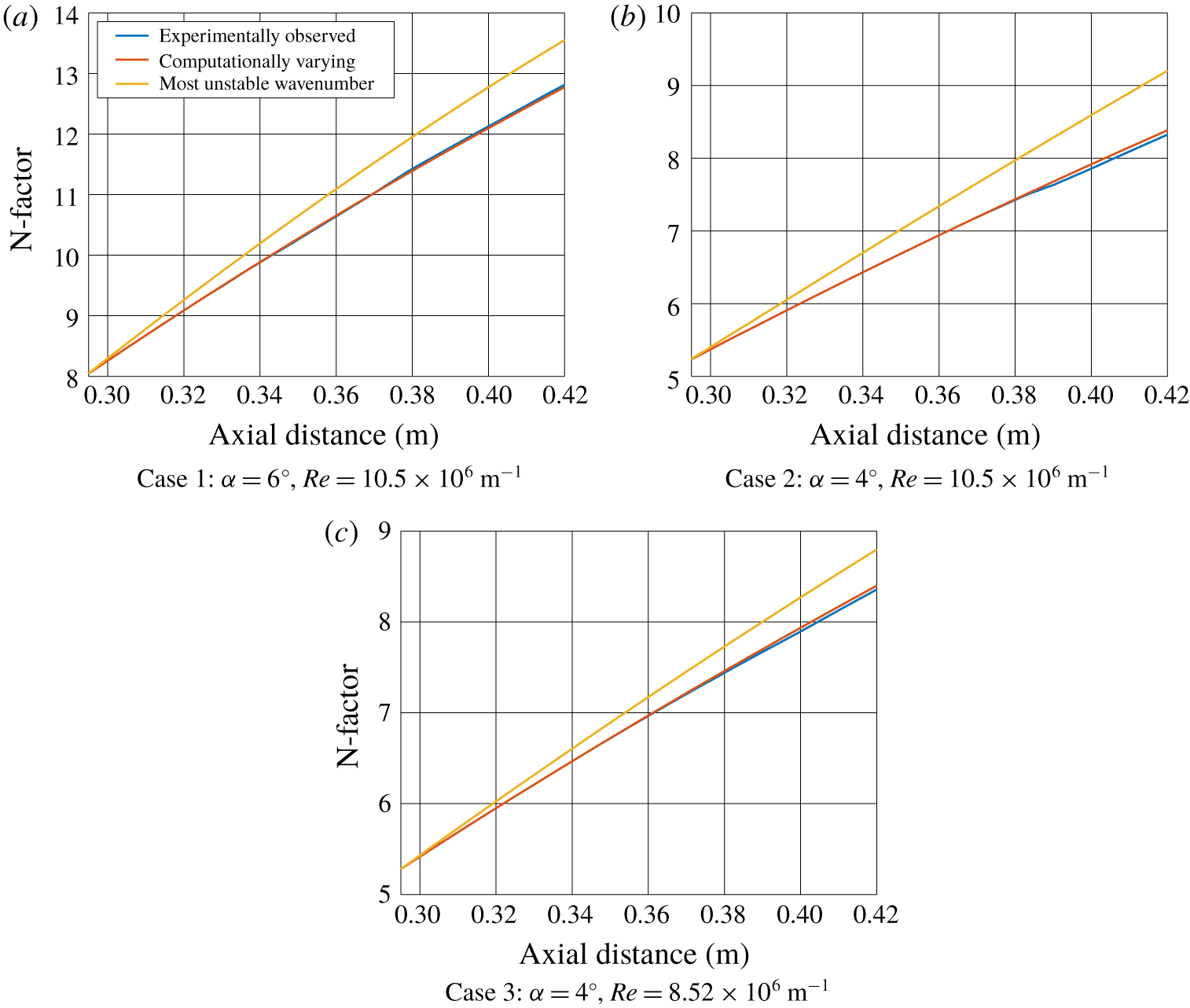
Figure 23 shows N-factors over the area with a defined experimental wavenumber. The first technique – selecting the most unstable wavenumbers – resulted in the N-factor at the end of the cone approximately 1 larger than the other two methods. The hybrid computational/experimental (‘computationally varying’) wavenumbers and the experimentally observed wavenumbers results in N-factors that matched closely. These behaviours were observed for each of the three test cases.
N-factors calculated with different wavenumber variations.

The similarity of N-factors for the hybrid computational/experimental and experimental-only wavenumber distributions suggests that either can be successfully employed in the stability analysis of a three-dimensional flow field. The hybrid method is a good choice if one has limited experimental data – for example, an FFT calculated for a spanwise heating distribution, or a set of discrete sensors at one axial station. The experimental-only method is good if one has a complete map of stationary cross-flow wavenumber evolution, but less sophisticated computational analysis of the vortex spreading. In contrast, using the computed most unstable wavenumbers introduces error into the calculated N-factor. The error is systematic and will always result in a too-large N-factor.
7 Conclusions
Experimental surface heat-flux data were collected on a  $7^{\circ }$ half-angle cone in the BAM6QT for varying Reynolds numbers at two angles of attack under quiet-flow conditions. The research focused on cross-flow-induced transition on the yaw side of the cone. A wavelet analysis was used to compute the local largest amplitude wavenumber of the stationary waves, which manifested themselves as hot streaks in the IR thermography surface heat-flux data.
The wavelet analysis provided a quantitative description of the spatial heat-flux distribution, presented as wavenumber. The wavenumber increased towards the leeward ray near the separation line and slightly near the windward ray for the  $6^{\circ }$ case. This behaviour was more pronounced as Reynolds number increased. The
 $4^{\circ }$ case resulted in more uniform wavenumbers compared to the
 $6^{\circ }$ case.
The wavelet analysis results were used to inform a stability analysis. N-factors were integrated along group velocity pathlines with the local wavenumber of the stationary cross-flow waves obtained three different ways. The traditional method, using the most unstable wavenumbers in the absence of experimental results, led to integrating amplification rates for wavenumbers that were not observed experimentally and relatively large N-factors. Global measurement of the wavenumber distribution is the most challenging because of the experimental and data reduction requirements. A hybrid method for computing cross-flow N-factors is recommended as the best path forward: compute the non-dimensional wavenumber ratios from group velocity pathlines and then dimensionalize them with experimental data. This would achieve very good agreement in N-factor with the experimentally more demanding method, but could better leverage results from literature, obtained with less comprehensive instrumentation, or for slightly different flow conditions.
Acknowledgements
This work was supported by the Air Force Office of Scientific Research under award number FA9550-16-1-0320. E. Heyse and M. Sanders of the Notre Dame Engineering Machine Shop consulted on the design and fabrication of the test model. M. Thompson, an undergraduate research assistant at Notre Dame, largely wrote the code used to process the IR camera images. C. Running, a Notre Dame graduate research assistant, supervised M. Thompson and consulted on the IR camera setup and data reduction. Professor S. Schneider, Purdue University, graciously allowed use of the BAM6QT. Dr B. Chynoweth, Dr J. Edelman and G. McKiernan trained H.Y. to run the tunnel and assisted in setting up the experiment.
Appendix. Direct measurement of distance between hot streaks
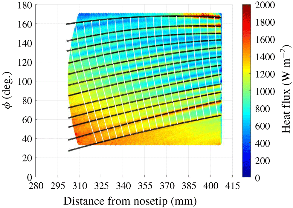
The most straightforward implementation of the wavelet analysis uses spanwise heat-flux profiles as the input, and thus the output wavelengths are normalized by the local radius of curvature of the cone’s circular cross-section at a given span. However, it would be more proper to determine the cross-flow vortex wavelengths normal to the vortex paths (Kuehl et al. Reference Kuehl, Perez and Reed2012) and normalize them by the local radius of curvature of the elliptical cross-section resulting from the conic section at an oblique angle to the axis. A second approach to evaluating the experimentally observed wavenumber distribution, which accounts for the curving vortex paths, was executed. The first step was to identify every hot-streak path in a heat-flux contour. The gradient of the surface heat flux along these paths was calculated to produce the vectors perpendicular to the hot streaks. Tangent lines connecting these perpendicular vectors were calculated in 1 mm increments. This technique resulted in the generation of lines perpendicular to the hot streaks resulting from the stationary cross-flow vortices. The length of each segment of the perpendicular lines was computed, giving a direct measurement of the local wavelength normal to the hot streaks. Figure 24 shows the IR heat-flux data from figure 10 with the vortex paths (black lines) and vortex-normal lines (white lines) superimposed on the heat-flux contours. All vortex paths are shown, but only 20 vortex-normal paths are included for clarity.
The IR heat-flux data with vortex paths and example vortex-normal paths identified.

Spatial mapping of stationary cross-flow vortex distribution using vortex-normal heat-flux profiles.

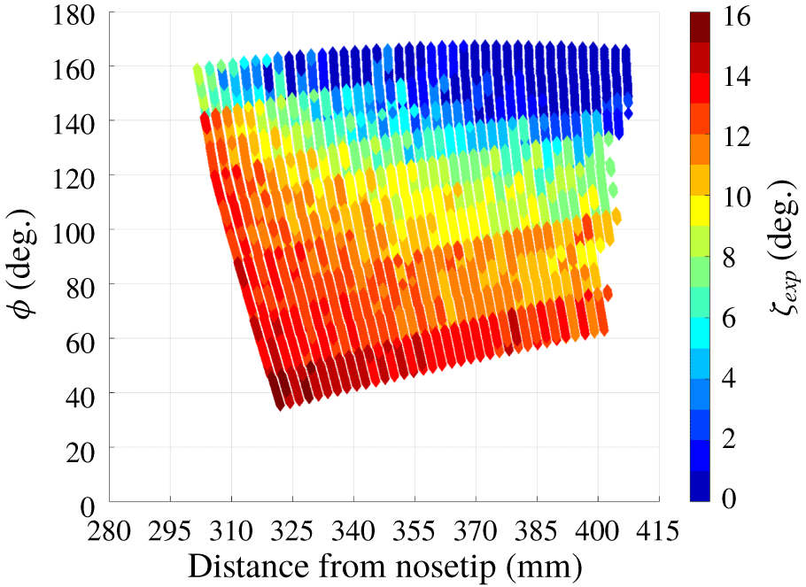
Angle of the stationary hot streaks relative to the cone axis.

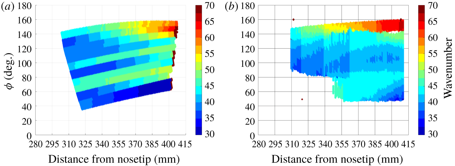
Comparison of spatial mapping of stationary cross-flow vortex distribution using wavelet analysis and vortex-normal heat-flux profiles.

A contour plot of the length of the perpendicular line segments functions as a map of the normalized wavelength or wavenumber for this technique. The wavelength was normalized by the local radius of curvature of the elliptical conic section created when slicing the cone along a vortex-normal path. Figure 25 shows the results using this technique. Note that in analysing the data from figure 24, the vortex path closest to the leeward ray has been ignored because the azimuthal position of this hot streak lies outside the region where the cross-flow instability is the dominant transition mechanism. The direct measurement technique computes the distance between two hot streaks. Thus, the results of using this technique on  $n$ hot streaks contain
 $n-1$ paths between them. Regions of high wavenumber are seen near the leeward ray of the model where the vortices converge due to the spanwise pressure gradient. The wavenumber generally increases moving downstream, except at the lowest azimuth. Figure 26 shows the computed angle of the hot streaks with respect to the cone axis. The angle of the hot streaks was seen to increase upstream and near the windward ray of the model. Values of
 $10^{\circ }$ or less were seen in the regions where the cross-flow instability is the dominant transition mechanism. This also agrees qualitatively with the behaviour of computationally generated inviscid streamline paths (Yates et al. Reference Yates, Juliano, Matlis and Tufts2018) and vortex paths (Li et al. Reference Li, Choudhari, Chang and White2010). The error introduced in the normalized wavelength or wavenumber by failing to account for an elliptic, not circular, radius of curvature, is small (approximately 0.5 %–2 %) in the region where stationary cross-flow vortices are most amplified. Therefore, the simplification of using spanwise heat-flux profiles normalized by a circular radius of curvature introduces minimal error.
Change in wavenumber between the wavelet and direct measurement techniques.

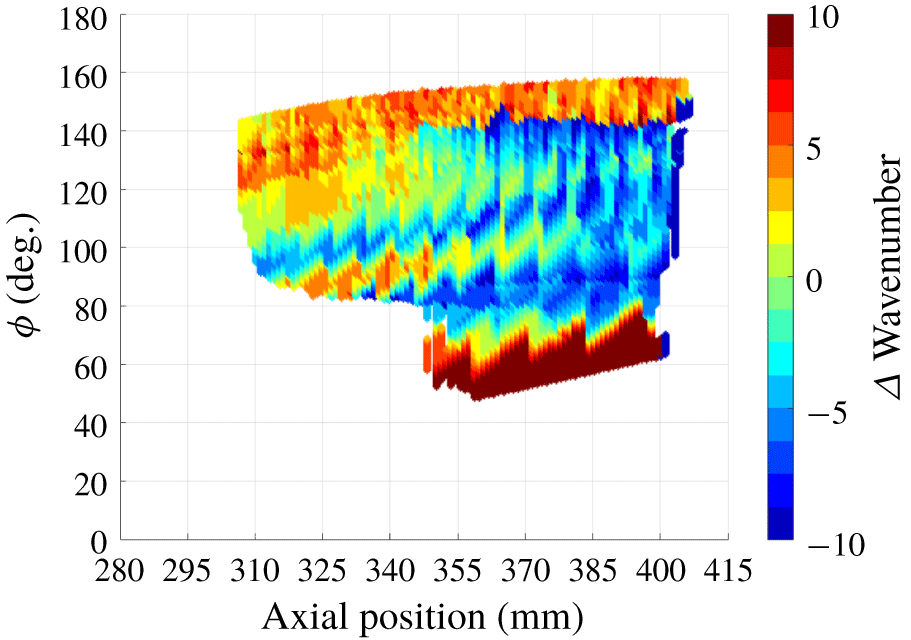
These results are similar to those from the wavelet analysis based on spanwise heat-flux profiles (figure 27). In both cases, a region of wavenumber greater than 50 is seen downstream near the leeward ray. A region of low wavenumber is seen closer to the windward ray, where stationary vortices were not observed in the experiment. Figure 28 shows the difference in wavenumber as indicated by these two techniques, where the data from figure 25 have been interpolated onto the mapping from figure 13. Due to the paths of the vortex-normal profiles and the cone of influence in the wavelet analysis, the regions where the wavenumber could be resolved differ slightly between the techniques. Figure 28 indicates that generally the results between the two techniques differ by a wavenumber of five or less, compared to a wavelength resolution of  $1.80^{\circ }$ for the wavelet results. The two techniques yield similar results over much of the region of interest. For example, a band of
 $k\approx 45$ at
 $\unicode[STIX]{x1D719}=70^{\circ }$, with minima above and below, was observed using both techniques. The largest differences were observed near the windward and leeward rays, where the wavelet analysis with spanwise profiles yielded higher wavenumbers.
The wavelet analysis is much less time consuming than the one tracking hot streaks because very little work is needed to prepare the images for input to the wavelet analysis. The wavelet analysis is more robust for the small amount of noise present in the data and the amplitude threshold automatically determines the range over which the results are valid. For these reasons, and because the difference between techniques was not large, the wavelet analysis technique is preferred.
A third, hybrid technique was considered: manually identifying the hot streak paths, extracting the heat-flux paths perpendicular to the hot streaks and calculating the wavelet analysis for those profiles. This method was found to combine the worst features of both methods – it was time consuming, but did not result in precise wavelengths – so it was not pursued.