

“The only function of economic forecasting is to make astrology look respectable” J.K. Galbraith
Introduction
It is fair to say that Professor Galbraith's views on economic forecasting are likely to command strong support even, or perhaps particularly, among economists. Many economists might, if asked, see economic forecasting as the bastard offspring of their subject born of a union between bad economic theory and the uncertain application of statistical techniques. And a wide range of commentators loses no opportunity to observe that forecasts are generally wrong, sometimes losing the logic of their arguments in the process. For example, about ten years ago, the Financial Times observed that economic forecasts were often least reliable when times were most uncertain. It is not clear how one is to know when times were most uncertain, except by observing that forecasts have large errors.
One might think that similar forecasting problems have been faced by life actuaries. For many years mortality rates of old people decreased slowly. Then, around 1980, the proportionate rate of decline increased sharply. Since this change was without precedent, a natural conclusion was that the pre-1980 pattern would soon re-establish itself. In fact, as we have seen, in more recent years the rate of decline of mortality rates has, if anything, accelerated. While we do not have anything to offer on how forecasts of mortality rates might be improved, if key economic time series behaved like mortality rates, the problems faced by those involved in economic forecasting would be much greater than they actually are.
Of course the reality is that both economic and actuarial forecasts are needed and this is perhaps why, despite the best efforts of their detractors, forecasters seem to be irrepressible. The question of course is not whether they are right or wrong but whether policy is better made, or products such as pensions are better constructed, with forecasts or without them.
One could imagine economic policy being set without forecasts. Indeed some work over twenty years ago (Weale et al., Reference Weale, Blake, Christodoulakis, Meade and Vines1989) looked at policy rules on the assumption that both interest rates and tax rates responded to the data but not to views about what was going to happen in the future. Slightly more recently, the Taylor Rule (Taylor, Reference Taylor1993) suggested a framework where the interest rate was set with reference to the current rate of inflation and the current output gap (although the current output gap cannot sensibly be estimated without a forecast and even with it can hardly be regarded as certain (see Orphanides & van Norden, Reference Orphanides and van Norden2005). But, since policy moves such as interest rate changes take some time to have an effect, it makes more sense to set policy not with reference to the current state of the economy but with reference to where it is expected to be or, more explicitly, where inflation would be expected to be at any given interest rate setting (Svensson, Reference Svensson1997a, Reference Svenssonb).
On the Monetary Policy Committee (MPC) we normally aim to set monetary policy so as to achieve the inflation target in two to three years’ time. This horizon was adopted because the Bank's analysis suggested that interest rate changes had their most powerful influence on inflation about two years after they were made. A degree of flexibility is needed because different types of inflationary shocks work through in different ways. For example, there are very good arguments that, after large cost shocks to a depressed economy, one should not rush to bring inflation back to target.
More generally, if the MPC aimed to achieve the inflation target too quickly, the process might well match that of someone trying desperately to adjust a shower to the right temperature. By failing to take account of the lag between turning the taps and variations in the temperature of the water that comes out, the bather is condemned to a sequence of water that is too hot followed by water that is too cold and so on. Only a degree of patience can deliver a comfortable shower.
Inevitably, if we aim to achieve our target at some time in the future we have to take account of where we might expect the economy and particularly the inflation rate to be in the absence of any change to economic policy. This can be done only by means of a forecast. Relying only on current information would be appropriate only if the current state of the economy were the best guide we have to the future. Historic evidence suggests that economic forecasts, despite the strength of Professor Galbraith's views, have more predictive power than the assumption that either the current rate of inflation or the current rate of economic growth would continue indefinitely (Pouzilac et al., Reference Pouzilac, Weale and Young1996).
So forecasts are needed in the making of policy. Given that they are needed, and that they influence policy setting, they should be in the public domain. But, given that they are in the public domain, it is important that producers of forecasts should help outside users of them understand their limitations. In particular, users need to understand that forecasts are simply the best that forecasters can do with the information available. Experienced forecasters know better than to claim that they are good at forecasting on the basis of one or two years of good luck.
A focus on the uncertainty surrounding a forecast rather than on a single trajectory is widely regarded as the most appropriate way of communicating the realities of forecasting, whether applied to the economy, to mortality or to any other variable. And there are very good reasons why such information is important both for policy-makers and for other users of forecasts. Businesses which insure people against the risk of longevity are much more likely to be concerned about unexpectedly low rates of mortality than about unexpectedly high rates of mortality. The former may result in the insurance company being unable to meet its promises while the latter lead to high profits for shareholders. While the latter might be welcomed, the former would put the business model at risk; one could hardly imagine a well-run business feeling that the two risks balanced out. Similarly, after a period like the recent past in which inflation has been above target for much of the time, it is easy to see why central bankers might be more concerned about inflation being above target at the relevant forecast horizon than about it being below target. The argument is that continuing above target inflation could lead to inflationary expectations becoming entrenched with the policy framework losing its credibility. On the other hand, if inflation were to be below target after a sustained period above target the public would be unlikely to think that the central bank had lost interest in its target or that an unmanageable deflation threatened. Rather they would think that these sorts of fluctuations were normal in the current choppy environment. But enough of the reasons why people need to know more about forecasts than simply being given forecast trajectories. We proceed to a brief account of how that has been done.
Presentation of Uncertainty
HM Treasury was probably the first body in the UK to indicate the uncertainty surrounding their forecasts. The 1976 Industry Act obliged them to publish their forecasts and, in 1979, they started to include tables showing the mean absolute errors associated with their forecasts. These tables could have done nothing except convey the (correct) impression that users, even if not themselves aware of the Treasury record, should not expect the forecasts to be accurate. It is questionable how far the presentation of mean absolute error rather than standard error is helpful because, should one want to use the information to parameterise a density function and then derive event probabilities such as the chance that output is stagnant or falling, this is more conveniently done in terms of a standard error. Wallis (Reference Wallis1999) explains that if policy-makers regard the costs of the failure to meet their targets as linear in the deviation of the outturn from those targets, then policy should respond to the median outcome and losses should be assessed with reference to the mean absolute deviation from target. But this does not translate into an emphasis on the mean absolute forecast error unless the only costs policy-makers were concerned about arose from being unable to predict the future state of the economy – a situation which seems most unlikely.
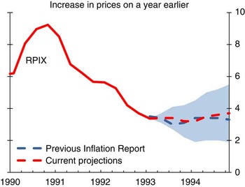
Other UK forecasters did not immediately follow the Treasury lead. However, in 1993, the Bank of England began to produce its Inflation Report. From then until November 1995 it published a chart like that shown in Chart 1 which presented the central forecast together with an indication of the mean absolute error. The Bank now provides the information needed to convert these charts into implied probability distributions “in the interests of science”.
May 1993 Inflation Report chart of RPIX inflation projections and outturns(a)
(a) Chart reproduced using parameters published on Bank of England website.

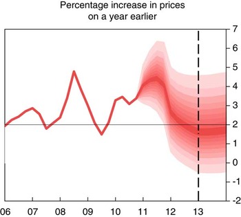
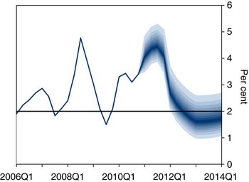
In February 1996, the Bank began the fan chart in its current format. There are two key differences between this and what was done between 1993 and 1995. First, the focus moved away from an analysis based on past forecast errors to one intended to represent the subjective view of the Bank.Footnote 1 Secondly, an explicit structure for the density function of forecast errors made it possible to depart from the assumption that risks are symmetric. By using a composite of two normal distributions (Gibbons & Mylroie, Reference Gibbons and Mylroie1973, Johnson et al., Reference Johnson, Kotz and Balakrishnan1994, page 173) in which the variance of the distribution above the central parameter could differ from that below the central parameter, it became possible to represent a degree of skewness. Of course, like the models used by the Committee to produce the central projection, this distribution is only a tool. It does not necessarily represent all Committee members’ view of the true distribution. But, as Britton et al. (Reference Britton, Fisher and Whiteley1998) noted in their explanation of the fan chart, the use of a distribution allows the Committee to represent the belief that the distribution of possible outcomes might not be symmetrically distributed about the central reference point without needing to consider the infinite combination of possible scenarios, from which the distribution might be drawn. The fan chart for inflation published in February 2011 is shown in Chart 2.
February 2011 Inflation Report chart of CPI inflation projections

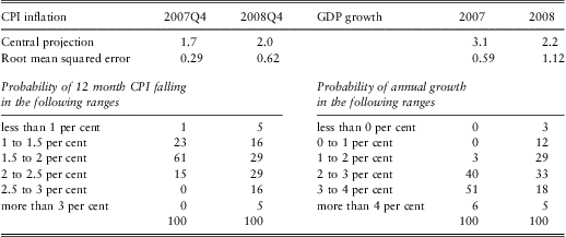
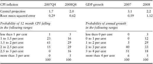
The National Institute did not publish regular information on its forecast errors until 1993. In April 1996, for the first time it evaluated the standard deviation of the forecast errors from its past record and used this to compute the probability that inflation and GDP growth would lie in particular ranges, so-called event probabilities. This was presented in tabular form as the example from October 2007 shows – see Table 1.
Event probabilities for inflation and GDP from the National Institute forecast for October 2007
In the late 1990s, work using stochastic simulations of its economic model suggested that a model-based analysis of forecast uncertainty gave results similar to one deduced from past forecast errors. This need not have been the case because, as every forecaster knows, forecasts reflect forecasters’ judgements as well as the models that they use. The requirement that the starting point of a forecast should be determined largely by data about the present means that there is no such thing as a pure model-based forecast.
It was unfortunate that the greater attention paid to forecast uncertainty by the National Institute, in combination with the Bank's approach, did not trigger a more general debate by economic forecasters about how best to represent uncertainty. However the National Institute's experience did demonstrate the pitfalls of relying on past forecast errors. In the 1970s and 1980s inflation was not only high but also volatile. The National Institute's forecasts of inflation in the 1970s and 1980s inevitably showed fairly large errors and these were translated into high probabilities of inflation being a long way from both the forecast and the Bank's target in the late 1990s. As we know inflation was in fact extraordinarily stable during this period with the result that the National Institute substantially over-stated the probabilities of inflation being a long way from its target. Thus a formal study (Mitchell & Hall, Reference Mitchell and Hall2005) showed that while the outturns for inflation were coherent with the Bank's fan-chart, their distribution was incompatible with the National Institute's view at that time about the uncertainty surrounding its forecast.
This experience has, of course, a more recent moral as Table 1 might hint. In 2008, GDP was in fact slightly lower than in 2007, something to which the National Institute forecast gave a probability of only three per cent. The problem was even worse in 2009 when the UK economy showed the largest contraction in output since 1921. An analysis based on recent forecast errors and the assumption of a normal distribution can understate the risk of relatively rare events.
Rare Events
This problem can be understood by asking how often one should expect to a recession. Over the last hundred years there have been six periods in which the output of the economy has been depressed below its previous peak, ignoring the distorting effects of the two world wars. So what is the risk of a recession starting? If we assume that a recession typically lasts for two years then there have been ninety-four years in which recessions might have started. The probability of a recession starting, given one is not already underway, is 6.4%. But this has a standard error of 2.5%. So a reasonable inference is that there is a one-in- eight chance of the probability of a recession being almost ten per cent. There must be some businesses which would pay more attention to the risk of recession if they thought there was a reasonable chance it could be a one-in-ten year event rather than if they assumed the risk was not much more than half of that.
To use more data is not necessarily a solution; the British economy before the First World War was very different from what it is today and I am not sure that we can learn an enormous amount about the frequency of the risks facing the contemporary economy from a study of Queen Victoria's reign. Indeed, although national accounting data exist for much of the nineteenth century exist, it is not clear that they are well-suited to identifying a modern economic cycle.
Could the problem be that the nature of the shocks has changed rather than that rare events have turned out to be less rare than thought? It is not clear how one might distinguish between the two or even that they are distinguishable. These problems have, of course, been appreciated by authors such as Basak & Shapiro (Reference Basak and Shapiro1998), Artzner (Reference Artzner1999) and Berkowitz (Reference Berkowitz2001) who have written on the problem of testing models of the probabilities of rare events. They point out that extra traction can be gained by looking at expected values conditional on thresholds being breached. Nevertheless, one cannot make a silk purse out of a sow's ear. If an event happens only very rarely then the expected loss conditional on that event will be very poorly determined. The probabilities of rare events must be highly uncertain and those who estimate such probabilities should make sure that they are described as such.
As both Mervyn King and Charlie Bean have noted in the past (King et al., Reference King, Aikman, Barrett, Kapadia, Proudman, Taylor, de Weymarn and Yates2010, and Bean, Reference Bean2010), to avoid a spurious degree of precision the MPC does not publish the details of the distribution of the shocks to which it thinks the economy might be subject outside the 10th and 90th percentiles (although of course it could not publish an expected value for the outcome without making some assumption about the tails of the distribution). But ducking the issue in this way does not completely avoid the problem because, as recent events have shown, possibilities which were regarded as highly unlikely might, nevertheless, happen. The distributions that it does publish can be disrupted if rare events turn out to be less rare than was thought.
Uncertain Probabilities More Generally
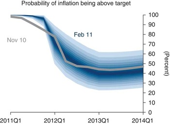
But it is not only with rare events that one might want to recognize that the probabilities are uncertain. Just as the Monetary Policy Committee does not want to draw attention to a single forecast path for the economy, so too it might feel uncomfortable about the idea that it could attach a precise probability to any particular event. A sense of this malaise can be gained from the Inflation Report. The Committee, reasonably enough, has felt the need to say what it thought was the probability that inflation would be above or below the two per cent target at some point in the future. A probability by its nature is a precise proportion. And a number like this could be calculated using an assumed probability distribution for the dispersion of risks surrounding the MPC's central projection.
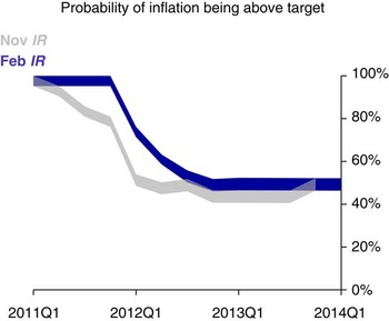
Nevertheless, as Mervyn King discussed in a speech at the Royal Statistical Society (King et al., Reference King, Aikman, Barrett, Kapadia, Proudman, Taylor, de Weymarn and Yates2010), the Committee feels that such precision is inappropriate; instead it shows Chart 3. The reader can infer from this that, in early 2011, the MPC thought that the probability inflation would be above target was close to 100 per cent and that, by late 2012, this probability would have dropped back to around 50 per cent. But it is not possible to give a precise definition either to the boundaries of the ribbons or to their interior points. The imprecision has its merits because probabilities are uncertain. Nevertheless, there may be other ways of conveying this uncertainty.
The ribbon chart, an indicator of the probability inflation will be above target (February 2011 Inflation Report)

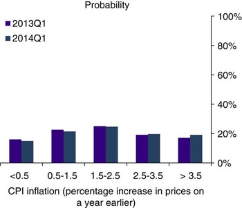
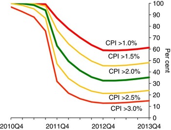
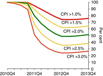
Some users of the Inflation Report certainly feel that the views of the Monetary Policy Committee on the uncertainties surrounding the inflation projection could be set out more clearly. For example Giles (Reference Giles2010) has made some helpful suggestions from which Chart 4 is derived. This indicates the probability that the Committee attaches to the inflation being above or below particular threshold values.
A chart showing probability that inflation will exceed certain thresholds (February 2011 Inflation Report)

Of course it could also be argued that users who want a chart like this can work it out for themselves as Giles has done based on the information provided about the two-part normal distribution. But that is hardly satisfactory. The Inflation Report should convey its message in the form most helpful to its readers. This does not, of course, mean that we should present what readers request if that might distort the message.
The question then arises whether Chart 4 does run the risk of distorting the message the Committee wish to communicate. Not surprisingly Giles is particularly interested in the probability that inflation is going to be below 1% or above 3%. These are of course the thresholds at which the Governor of the Bank of England has to write to the Chancellor. But the Committee has a point target and presenting ranges based on the 1% and 3% threshold may confuse the public into either misinterpreting the Committee's target or into believing that an inflation rate of slightly more than 3% is significantly worse than one of exactly 3%, which is not true. And the Committee does already provide more information on the probabilities of inflation being significantly away from target using illustrations such as Chart 5. Nevertheless, we consider here the probabilities of inflation being below 1% or above 3% because these ranges are significant departures from the 2% target.
Frequency distribution of CPI inflation in February 2011 Inflation Report based on market interest rate expectations and £200 billion asset purchases

More importantly, as with the earlier discussion of the chance of inflation being above or below target, a diagram like Chart 4 would probably convey a precesion which the MPC might feel did not accurately represent its views. So the question addressed here is whether there are ways in which the MPC could helpfully represent the uncertainty it might feel about the uncertainty facing the economy? Söderlind & Svensson (Reference Söderlind and Svensson1997) discuss this issue in the context of using option prices to extract a market view about the probability distribution of future asset prices. But it is not central to their paper and has not, so far as we are aware, received a great deal of attention since then.
Multiple Sources of Uncertainty
One reason why there may be uncertainty about the probabilities is that the parameters of the two-part normal density function are themselves uncertain. Perhaps an easy way to think of this is that there is a large number of plausible forecasts, generated from a range of different models and, indeed a range of different people with different views.Footnote 2 Each of these forecasts has a density function associated with it. So each forecast could generate its own fan chart and the uncertainty about the probabilities arises from the reality that we are uncertain which fan chart to use.
Before looking at the implications of such a situation for uncertainty about probabilities, something needs to be said about how one might generate an overall fan chart in such a situation. Wallis (Reference Wallis2005) drew on the literature associated with mixed distributions (see also Hall and Mitchell, Reference Hall and Mitchell2007). Smith & Wallis (Reference Smith and Wallis2009) provide a statistical analysis which indicates why using equal weights to combine distributions might be a sensible choice. If this is applied to a situation where there are is a small number of possible density functions, generated by competing models, then the principle is clear enough.
If, however, there is a large number of possible models, verging on a continuum with its own density function, then there is a case for weighting the density function generated at each point on the continuum by the probability associated with it. Such a situation might arise if, for example, there were a range of central forecasts and each had a shock around it. If both the forecasts and the shocks were normally distributed, and the latter were independent of the model to which they related and had a known variance, then the resulting overall density function would also match a normal distribution. So in such a situation it would be easy to generate a combined fan chart. But the uncertainty about the probabilities arises from the uncertainty surrounding the parameters of the forecast as a concrete example illustrates. Uncertainty about the appropriate model is a known unknown and the effects of subsequent shocks are unknown unknowns.
Suppose that we were 50% confident that, in the absence of shocks, the inflation rate would lie between 2.4% and 2.7% at some point in the future. And we also assumed that the standard deviation of inflation as a result of unforecastable shocks was 1%. If the rate in the absence of shocks was 2.4%, the probability that inflation would exceed 3% is 27% while an unperturbed rate of 2.7% leads to a probability of exceeding the 3% threshold of 38%. So in this example, instead of giving a precise probability of inflation being 3% or more, the Committee might wish to say that it was 50% confident that the probability lay between 27% and 38% or perhaps even more generally that it was moderately confident that the risk lay between 25% and 40%. This sort of presentation could convey the air of uncertainty surrounding the forecast better than would a single probability – and the benefits to be gained from this sort of approach might be thought to more than outweigh the disadvantage that the model of risks is more complicated than is used at present.
How far should this be taken? If we are to talk about uncertainty surrounding the central value of the distribution one might reasonably well ask whether we should be concerned with uncertainty surrounding the shocks? One might, for example, want to assume that the variance is itself distributed as a χ2 variable with some assumed number of degrees of freedom. Indeed Teichroew (Reference Teichroew1957) sets out the resulting overall distribution if that is the only source of uncertainty. But a moment's thought shows that uncertainty about the variance leads, on its own, to very considerable uncertainty about the extreme probabilities, but none at all about the median. Thus it is not satisfactory to rely solely or mainly on uncertainty about the variance as a way of representing the uncertainty about probabilities of particular events. Similarly there is probably not much to be gained from worrying about the uncertainty of the skew parameter.
There is a separate question whether the parameters of the density function associated with each of the possible models should be assumed to be related to the parameters of these models. Obviously, when fitted to past data, some models do well and others do badly. But, for the purposes of conveying uncertainty about uncertainty, this is probably not so important as to justify departing from the simple assumption that all forecasts have the same error density function associated with them.
Finally, there is a separate question whether it makes sense to assume that the disturbances associated with each particular forecast in the density function are independent of that forecast. This is an issue which merits further thought; for the time being we have assumed independence. With this structure in mind we can turn to the sort of representations of uncertain uncertainty that a body like the MPC might produce.
Application to the Fan Chart
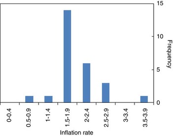
In order to illustrate uncertain uncertainty, we have assumed that the dispersion of underlying models can be deduced from the spread of independent inflation forecasts for the final quarter of 2012 as collected by the Treasury late in February 2011. This is shown in Chart 6.
Independent inflation forecasts for 2012 Q4

This chart is in some sense comforting for the MPC. Despite the current elevated inflation rate, it shows that the modal value for inflation in nearly two years time is under 2 per cent. But there are some other features of the distribution which make it of considerable interest. The mean value of the forecasts is 2.06 per cent. And, as the figure makes clear, the distribution is anything but symmetric. It shows a clear skew to the right. If the two-part normal distrbutionFootnote 3 adopted to describe the distribution of possible outcomes in the inflation report is fitted to these data, then the mode is just under 1.9 per cent with the standard deviation parameter for points below and above the mode equal to 0.40 and 0.6 respectively. This analysis where the mode is 0.16 percentage points below the mean can be compared with the February 2011 forecast produced by the Monetary Policy Committee which shows the mode to be 0.4 percentage points below the mean. Chart 7 shows a fan chart for the modal forecast on the assumption that the mode has the distribution represented by the two-piece normal distributionFootnote 4 fitted to the forecasts of Chart 6.
An example of an uncertain modal forecast of inflation

To build up an overall distribution from the combinantion of uncertainty about the model and uncertainty this two-piece normal distribution is used to represent the range of possible modal forecasts that might be envisaged by the MPC. We add to the modal forecasts represented by that distribution shocks, which are assumed to be normally distributed. The variance of this shock is chosen so that the overall variance of the combined density forecast matches that assumed by the MPC.
A consequence of this is that the skewness of the resulting fan chart is much lower than that adopted by the MPC. The skewness depends on the difference between the standard deviations of the left and right components of the two-piece normal distribution. But, with independence of shocks, it is the variances and not the standard deviations of the two distributions which are added together. This has the effect of reducing the gap between the standard deviations of the combined distribution below that of the initial two-piece normal distribution.
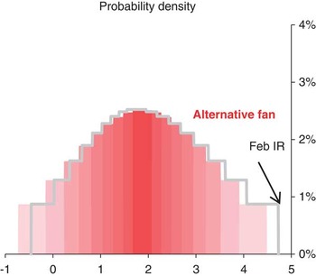
This means that adding on a symmetric disturbance to a skewed distribution like that used in the current fan chart has the effect of reducing the overall skewness of the combined distribution. Chart 8 and Chart 9 show histograms of the existing fan chart and the fan chart generated with the above assumptions nine and thirteen quarters into the forecast. Could any forecaster feel that one of the distributions in Chart 8 or Chart 9 is right and the other wrong, or vice versa?
Histogram of inflation forecasts in 2013Q1 derived from February 2011 Inflation Report and possible new distribution

Histogram of inflation forecasts in 2014Q1 derived from February 2011 Inflation Report and possible new distribution

Representation of Uncertain Uncertainty
Given the assumption that the central forecast has a skewed, two-part normal distribution, while the shocks around that most likely outcome are symetrically distributed the probabilities can be represented as uncertain. Chart 10 shows the probability that inflation is going to be above target and is an alternative way of presenting what was shown in Chart 3. This suggests a margin of uncertainty around the probability considerably greater than that indicated by Chart 3 possibly suggesting that the latter is not a good way of indicating that the event probabilities associated with the MPC's inflation forecasts are uncertain.
Replacement ‘ribbon’ chart

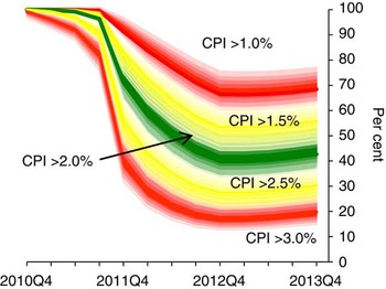
The implications of this approach for charts derived from those suggested by Chris Giles can also be considered. One way of doing this is to show two charts representing the 25th and 75th percentiles. This is done in Chart 11 and Chart 12.
Probabilities when the mode is drawn from the 25th percentile

Probabilities when the mode is drawn from the 75th percentile

These charts have to be considered together. They allow us to read off, for example, that there is a 50% chance that the probability of inflation being above 3% in 2013Q4 is between 15% and 26%. But processing information can be costly for the receiver, and the fact that the charts have be read jointly might place too much of the processing burden on the reader and lead to confusion about the message. This highlights the risk of releasing too much information in an unfiltered way – as Mervyn King put it: ‘less can be more’ (King et al., Reference King, Aikman, Barrett, Kapadia, Proudman, Taylor, de Weymarn and Yates2010).
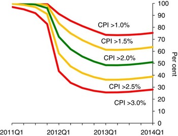
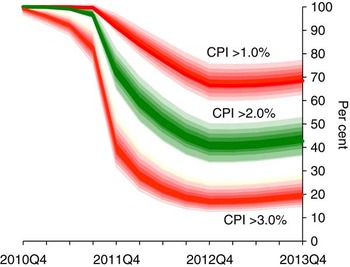
An alternative presentation is that shown in Chart 13. Here the two charts blur into one another so that, for example, the 50% probability range for the probability that inflation is above 1% lies in the upper fan, which shades from slightly red to solid red and back again. Similarly, the probability that inflation will be above  $$$1\tfrac{1}{2} $$$ per cent lies in the upper yellow fan, which shades from slightly yellow to solidly yellow. This is probably a more satisfactory way of conveying the uncertainty surrounding the probabilities.
Probability charts with the bands blended together to reflect uncertainty about the mode

There is, nevertheless, one problem associated with Chart 13. The chart shows only the percentiles comprising the central 50% of the distribution of the probabilities. But even these overlap; if the future became more uncertain this problem would become worse. One solution would be to leave out the yellow parts, showing simply the green centre, for the range of probabilities that inflation will be at target, and the red parts. Even greater uncertainty might mean that only the red parts could be shown without any confusion. For this reason it is probably desirable to include Chart 11 and Chart 12 as well as Chart 13 or Chart 14.
Alternative version of Chart 13 where yellow bands are omitted

Of course these are not the only charts representing probabilities in the Inflation Report. If desired it would also be possible to produce versions of the frequency distributions of inflation and growth at particular dates in a way which reflects the uncertain nature of such distributions.
A Coarser Fan-Chart
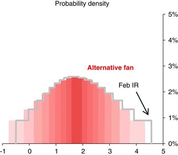
An alternative means of presenting the fan charts (e.g. Chart 2), in a way which would at least avoid the sense of precision conveyed by our existing charts is to show a much coarser representation of the distribution. The current fan charts represent deciles of the MPC's subjective distribution, with the outmost five per cent at the top and bottom of the distribution not shown. This means that, because the central decile is shown as a single band, seventeen bands can be identified in the fan charts published in the Inflation Report. In contrast the Office for Budget Responsibility shows only seven bands, with the central band representing a twenty per cent probability and each subsequent band a ten per cent probability on each side of the centre. The outermost twenty per cent of the distribution is not shown. Similarly Norges Bank shows only seven bands in its fan charts while the Riksbank offers an even coarser fan chart displaying the central fifty per cent, the bands on each side of this which together represent twenty-five per cent of the distribution and two further bands which together represent fifteen per cent of the distribution. An example of how a chart with seven bands might appear is provided in Chart 15 for comparison with Chart 2.
An inflation fan chart for February 2011 with coarse bands

There is much to be said for this as a means of avoiding the impression that the distribution is known with great accuracy. Users are expected to, and may well infer this because the distribution is coarse. It would however not be possible to draw graphs like charts 9 to 13. With this approach it would, however, be possible to make statements of the form that the probability of inflation being above target is thought to lie between x and y per cent.
Policy-Making
Where does this leave the practical problem that MPC members face in deciding how to set interest rates? On the one hand the future is uncertain – that is the the nature of the future. But on the other hand we need to come to a conclusion and each of us needs to cast a vote each month. We do not have the luxury of being able to spread our votes between different choices.
Chart 6 does indicate why there might be a divergence of views in the Committee with different people voting in different ways even though we can agree that something like Chart 7 represented our collective judgement. And MPC members are expected to vote in the light of their own views and not of the collective judgement.
Conclusions
Over the years since it was first published, the Inflation Report has set standards for the presentation of uncertainty. A key feature of the report has been a reluctance to suggest precision where that precision cannot be justified and for this very good reason the details of the central forecast are not published in the Inflation Report but are released one week afterwards. The Monetary Policy Committee has tried to draw attention to risks and uncetainty. And the success with which it has done this is demonstrated by the pressure for clearer information on the probabilities of particular outturns. But this in itself suggests a degree of precision with which at least this member of the Committee feels uncomfortable.
We have therefore endeavoured to set out here a framework which breaks the uncertainty in the forecasts of the Inflation Report into two components, one which might be thought associated with uncertainty about the central path and the other which might be linked to the shocks that can hit the economy. This makes it possible both to explain why the probabilities of particular events are uncertain and to replace precise probabilities with ranges. At the same time, it is important to acknowledge the practice adopted by other bodies of publishing coarser fan charts. These rely on users’ interpretation of them to communicate uncertainty.
But, if nothing else, this exercise has drawn your attention to the importance of communicating uncertainty as clearly as possible. Astrologers, as well as economic forecasters ought to attempt this.
Acknowledgements
We would like to thank both Ken Wallis and colleagues at the Bank of England for comments on earlier drafts. The views expressed are our own and do not necessarily reflect those of the Bank of England or other members of the Monetary Policy Committee.
Summary of the Discussion following Dr Martin Weale's Address, Uncertain uncertainty, to the Institute and Faculty of Actuaries, 29 March 2011, London
The President introduced Dr Weale as a distinguished Honorary Fellow of the Institute and Faculty of Actuaries who has been a member of the Monetary Policy Committee since last autumn. Dr Weale was Director of the National Institute of Economic and Social Research for 15 years and, prior to that, he was a lecturer in economics and a Fellow of Clare College at the University of Cambridge. The importance of his contribution to economics was widely recognised in 1999 when he was appointed a CBE for services to economics.
The President noted that actuaries and economists face a common challenge in analysing and communicating uncertainty, so the topic of Dr Weale's address was most appropriate. It was the President's experience that humility is the best form of risk management: there is a limit to how accurate risk can be modelled and there must be a willingness to learn to live with the residual inherent uncertainty. Donald Rumsfeld described the uncertainty well, as “unknown unknowns”.
The Actuarial Profession, opined the President, allowed its modelling in the last few decades to be interpreted as making predictions instead of being candid and taking the time to communicate the associated uncertainty. The reputational bruising that the Profession got when things worked out other than predicted was, in part, due to this.
The President opened the discussion to the floor. There followed a question and answer session.
The first question centred on whether, in forecasting inflation, a distinction should be made between inflation caused by price rises through scarcities of commodities and inflation caused from people's expectations of future inflation. The questioner believed that inflation caused by priced rises when some commodities become scarcer might be more difficult to constrain than the expectations that individuals have about the way prices are going to change over the next 12 months.
Dr Weale answered that the lessons of the sharp increase in oil and other commodity prices in 1973 initiated inflation which then got built in to pay bargaining in the UK. Germany, he pointed out, was exposed to the same sort of commodity price increase but the pay bargaining arrangements they had did not give rise to the same level of inflation. He pointed out that the Monetary Policy Committee (MPC) cannot control commodity prices, but it can attempt to stop that initial impetus causing pay bargainers and price setters too build in an expectation of a faster increase in prices. A tight monetary policy in these circumstances might keep overall inflation reasonably low and therefore inflation expectations muted so that, after the initial commodity-risen inflation, there is no further impact on people's real incomes.
One questioned the appropriateness of the definition of inflation. In particular, it was suggested that the recent crises may have in part been caused by a very large growth in the money supply which fed through into asset inflation, in particular the prices of houses, and that this was not at the time recognised as being a significant problem because house prices are not a feature in the official definitions of inflation.
Dr Weale pointed out that there is, of course, a fundamental problem in having a single indicator attempt to capture what is happening to the multitude of prices in the economy. There are many ways to reduce the thousands of prices to a single indicator, each having its own strengths and weaknesses. The consumer prices index is trying to measure the cost of things as people are using them up. When a house is bought it is not used up, so you would not expect housing to enter into a consumer prices index in the way that a loaf of bread enters into the index. He noted that there are substantial discussions about the most appropriate way of putting housing into the index but, nothwithstanding that, he was of the opinion that movements in house prices would not have a big impact on the Consumer Prices Index. Issues of house price inflation and asset price inflation, to the extent that they are a policy concern, need to be addressed separately, he concluded.
A visitor pointed to Chart 14, which shows the distribution around event probabilities assuming forecasters are independent of each other, and asked whether those distributions should actually be a lot wider in the circumstance that many forecasters follow a the Bank of England's forecasts and so are not really independent.
Dr Weale conceded that the answer to this point is not straightforward and he would like to think further on it. His initial thought was that another way of getting some sense of dispersion was to simulate with a wide range of models, but probably what comes from a model depends on the input for expectations of future inflation, and that is a bit circular.
Another contributor asked whether in some circumstances future inflation might be near a phase change – so say, it might be 2% or 4% but it is unlikely to be in between them – and asked how that sort of uncertainty could be represented.
Dr Weale answered that that did not present a conceptual problem – the answer can be found in many statistics books and, if he recalls correctly, the diagram capturing the uncertainty looks like a camel with two humps. However, on a related point, he expressed scepticism when someone opines that the economy is on a precipice or things will suddenly flip. He conceded that they could be right, like in late 2008, but much more often they are wrong: he hears such forecasts with remarkable frequency relative to the extent to which it happens.
Another mischievously asked why anybody should assume that the centre part of the distribution of future inflation forecasts published by the Bank of England is in the right area. He wondered why there should be much confidence in these forecasts when the Bank had missed the inflation target so often in the past.
Dr Weale pointed to three things that are particularly difficult to forecast and can have a significant impact on inflation out-turns: future tax changes, commodity prices, and movements in the exchange rate.
The MPC takes account of future tax changes only if they have been announced. The recent VAT increase added something between 1 and  $$$1\tfrac{1}{4}$$$ percentage points to the inflation rate as of January or February. So, without further tax surprises, the MPC should do better in the future than in the recent past.
Commodity price rises and the aftermath of depreciation of the pound are other forces, quite difficult to forecast, leading to inflation being higher of late than the central forecast. He said that it would be nice not to live in such an uncertain world, and the world seems to be at the moment more volatile than previously, but the MPC are trying to reflect that explicitly by showing uncertainty in the forecasts.
An actuary working in general insurance asked how one might helpfully communicate uncertainty out in the extremes – uncertainty around one-in-200 events and more extreme events than that.
Dr Weale suggested that, as it was difficult to estimate the true probability of an extreme risk, he would want to build a substantial margin of error, which translates to larger risk reserves than if you could estimate with certainty exactly what is a one-in-200 year event.
The President brought the evening to a close. He suggested that the address will have replenished the courage of actuaries to embrace uncertainty, not to pretend that it does not exist, and to be better prepared to go to their clients and accept that there is uncertainty and work with them to manage it.