2 Equations solved by stella and GENE

The codes $\texttt {stella}$ and $\texttt {GENE}$ are based on the $\delta f$ gyrokinetic theory, first proposed in Catto (Reference Catto1978). In the present paper, we use versions of these codes that solve the flux-tube gyrokinetic equations for stellarator electrostatic turbulence. The flux-tube approach explicitly exploits the scale separation between the typical variation lengths of the background magnetic field and plasma profiles, and the typical spatial scales of the turbulent fluctuations in the plane perpendicular to the magnetic field. Next, we introduce the coordinates used along the paper and write the electrostatic flux-tube equations.

We consider stellarator configurations with nested magnetic surfaces and define spatial coordinates $\{r, \alpha, z\}$, where $r\in [0,a]$ is a radial coordinate that labels magnetic surfaces, $\alpha \in [0,2{\rm \pi} )$ is an angular coordinate labelling field lines on each magnetic surface and $z \in [z_{\mathrm {min}},z_{\mathrm {max}}]$ is a coordinate along field lines. Here, $a$ is the stellarator minor radius. The value $r = a$ corresponds to the last closed flux surface.Footnote ¹ Specifically, we choose

(2.1)\begin{equation} r:= a\sqrt{\frac{\psi_t}{\psi_{t,a}}}, \end{equation}

where $2{\rm \pi} \psi _t(r)$ is the toroidal flux enclosed by the surface labelled by $r$ and $\psi _{t,a}:=\psi _t(a)$. As for $\alpha$, we take

(2.2)\begin{equation} \alpha=\theta-\iota\zeta, \end{equation}

where $\theta$ and $\zeta$ are, respectively, the poloidal and toroidal PEST flux coordinates (Grimm, Dewar & Manickam Reference Grimm, Dewar and Manickam1983) and $\iota (r)$ is the rotational transform. In these coordinates, the magnetic field can be expressed as

(2.3)\begin{equation} \boldsymbol{B}=\psi'_t\boldsymbol{\nabla} r\times \boldsymbol{\nabla} \alpha. \end{equation}

Throughout the paper, a prime $(')$ means differentiation with respect to $r$. Note that, with our choice for $r$, we have

(2.4)\begin{equation} \psi'_t(r) = \frac{2\psi_{t,a} r}{a^{2}} . \end{equation}

It is also useful to define the quantity $B_a$, which will be used in this paper as a reference magnetic field and it is given by

(2.5)\begin{equation} \psi_{t,a} = \mathrm{sgn}(\psi_{t,a})\frac{a^{2}B_a}{2}, \end{equation}

where $\mathrm {sgn}(\cdot )$ is the sign function, so that $B_a$ is always positive.

Let $r_0$ and $\alpha _0$ be the values of $r$ and $\alpha$ that select a flux tube (and the centre of the simulation domain). In the plane perpendicular to $\boldsymbol {B}$, $\texttt {stella}$ and $\texttt {GENE}$ use coordinates $x$ and $y$ defined as

(2.6)\begin{equation} x: = r -r_0 \end{equation}

and

(2.7)\begin{equation} y: = r_0(\alpha -\alpha_0), \end{equation}

whereas, along $\boldsymbol {B}$, $\texttt {stella}$ takes $z = \zeta$ and $\texttt {GENE}$ employs $z = \theta$. In velocity space, stella and GENE use $v_{\|}$ and $\mu$ as independent coordinates, where $v_{\|}$ is the component of the velocity parallel to the magnetic field line and $\mu =m_jv_{\perp }^{2}/2B$ is the magnetic moment, with $v_{\perp }$ the component of the velocity perpendicular to the magnetic field, $|\boldsymbol {B}| = B$ the magnetic field strength and $m_j$ the mass, where the subscript $j$ indicates the species. Here, $j$ can take the values ‘$i$’, if it refers to ions, and ‘$e$’, if it refers to electrons. In coordinates $\{x, y, z, v_{\|}, \mu \}$, the fluctuating distribution function of the species $j$ can be Fourier expanded as

(2.8)\begin{equation} g_j(x, y, z, v_{\|}, \mu, t) = \sum_{k_x, k_y} \hat{g}_{\boldsymbol{k}_{{\perp}},j}(z, v_{\|}, \mu, t)\exp({\mathrm{i}(k_x x +k_y y)}) \end{equation}

and, equivalently, the fluctuating electrostatic potential can be expressed as

(2.9)\begin{equation} \varphi(x, y, z, t) = \sum_{k_x, k_y} \hat{\varphi}_{\boldsymbol{k}_{{\perp}}}(z, t) \exp({\mathrm{i}(k_x x +k_y y)}), \end{equation}

where $t$ is the time. The flux-tube gyrokinetic equation for the mode $\boldsymbol {k}_{\perp }$ of the fluctuating distribution function, $\hat {g}_{\boldsymbol {k}_{\perp },j}$, reads

(2.10)\begin{align} & \partial_t\hat{g}_{\boldsymbol{k}_{{\perp}},j} +v_{\|}\boldsymbol{\hat{b}}\boldsymbol{\cdot}\boldsymbol{\nabla} z\left(\partial_z\hat{g}_{\boldsymbol{k}_{{\perp}},j}+ \frac{Z_je}{T_j}\partial_{z}\left[\hat{\varphi}_{\boldsymbol{k}_{{\perp}}}{\rm J}_0({k_{{\perp}}v_{\bot}/\varOmega_j})\right]F_{0,j}\right) -\frac{\mu}{m_j}\boldsymbol{\hat{b}}\boldsymbol{\cdot}\boldsymbol{\nabla} B\partial_{v_{\|}}\hat{g}_{\boldsymbol{k}_{{\perp}},j}\nonumber\\ & \quad -\mathrm{i} {{\frac{\mathrm{sgn}(\psi_{t,a}) k_{y}}{B_a}}}\left[\frac{n'_j}{n_j}+\frac{T'_j}{T_j}\left(\frac{m_j(v_{\|}^{2}/2+B\mu/m_j)}{T_j}-\frac{3}{2}\right)\right]\hat{\varphi}_{\boldsymbol{k}_{{\perp}}}{\rm J}_0({k_{{\perp}}v_{{\perp}}/\varOmega_j})F_{0,j} \nonumber\\ & \quad+\frac{\mathrm{i}}{\varOmega_{j}}\left(v_{\|}^{2}\boldsymbol{\hat{b}}\times\boldsymbol{\kappa}+\frac{\mu}{m_j}\boldsymbol{\hat{b}}\times\boldsymbol{\nabla} B\right)\boldsymbol{\cdot}\boldsymbol{k}_{{\perp}}\left(\hat{g}_{\boldsymbol{k}_{{\perp}},j}+\frac{Z_je}{T_j}\hat{\varphi}_{\boldsymbol{k}_{{\perp}}}{\rm J}_0({k_{{\perp}}v_{{\perp}}/\varOmega_j})F_{0,j}\right) - N_{\boldsymbol{k}_{{\perp}},j} =0, \end{align}

where $B_a$ is given by (2.5), $n_j(r)$ and $T_j(r)$ are the density and temperature, assumed to be flux functions, $\varOmega _j=Z_jeB/m_j$ is the gyrofrequency, $Z_j$ is the charge number, $e$ is the proton charge, $\boldsymbol {k}_{\perp }=k_{x}\boldsymbol {\nabla } x + k_{y}\boldsymbol {\nabla } y$ is the perpendicular wavevector,

(2.11)\begin{equation} F_{0,j}=n_j(m_j/2{\rm \pi} T_j)^{3/2}\exp[{-}m_j(v_{\|}^{2}/2 + \mu B/m_j)/T_j] \end{equation}

is a Maxwellian and ${\rm J}_0$ is the zeroth-order Bessel function of the first kind. Finally, $\boldsymbol {\kappa }=\boldsymbol {\hat {b}}\boldsymbol {\cdot }\boldsymbol {\nabla }\boldsymbol {\hat {b}}$ is the curvature vector, with $\boldsymbol {\hat {b}}=B^{-1}\boldsymbol {B}$ and $N_{\boldsymbol {k}_{\perp },j}$ is the mode $\boldsymbol {k}_{\perp }$ of the nonlinear term, which can be written as

(2.12)\begin{equation} N_{{\boldsymbol{k_{{\perp}}}},j} ={\frac{\mathrm{sgn}(\psi_{t,a})}{B_a}} \sum_{\underset{k_{x_2}, k_{y_2}}{k_{x_1}, k_{y_1}}}{\left(k_{x_1}k_{y_2} - k_{x_2}k_{y_1}\right)}{\rm J}_0\left({k_{\perp_1}v_{{\perp}}/\varOmega_j}\right)\hat{\varphi}_{\boldsymbol{k}_{\perp_1}}\hat{g}_{\boldsymbol{k}_{\perp_2},j}, \end{equation}

where $\boldsymbol {k}_{\perp _1} = k_{x_1}\boldsymbol {\nabla } x + k_{y_1}\boldsymbol {\nabla } y$ and $\boldsymbol {k}_{\perp _2} = k_{x_2}\boldsymbol {\nabla } x + k_{y_2}\boldsymbol {\nabla } y$ are such that $\boldsymbol {k}_{\perp _1} + \boldsymbol {k}_{\perp _2} = \boldsymbol {k}_{\perp }$. The quasineutrality equation reads

(2.13)\begin{gather} \sum_j\frac{Z_jB}{m_j}\int_{-\infty}^{\infty}\,{\rm d} v_{\|}\int_0^{\infty}\,{\rm d}\mu {\rm J}_0({k_{{\perp}}v_{{\perp}}/\varOmega_j})\hat{g}_{\boldsymbol{k}_{{\perp}},j} \nonumber\\ +\sum_j \frac{Z_j^{2} e n_j}{2{\rm \pi} T_j}\left(\varGamma_0\left({\frac{k_{{\perp}}^{2}v_{{\rm th},j}^{2}}{2\varOmega_j^{2}}}\right)-1\right)\hat{\varphi}_{\boldsymbol{k}_{{\perp}}} = 0, \end{gather}

where $v_{{\rm th},j}=\sqrt {2T_j/m_j}$ is the thermal speed and $\varGamma _0(b)=\exp (-b){\rm I}_0(b)$ with ${\rm I}_0$ the zeroth-order modified Bessel function of the first kind. In (2.10) and (2.13), geometric quantities, as well as the plasma profiles and their derivatives, are evaluated at $r_0$ and $\alpha _0$. Both stella and GENE read the geometric quantities required to solve the gyrokinetic equations from a VMEC output.

Despite solving the same (2.10) and (2.13), there are some differences between stella and GENE when implementing them. We will only mention the most relevant ones and refer the reader to Barnes et al. (Reference Barnes, Parra and Landreman2019) and Merz (Reference Merz2009) for further details. The main difference is the treatment of the parallel streaming and acceleration terms in (2.10). For electrons, these terms of the gyrokinetic Vlasov equation scale up to a factor $\sqrt {m_i/m_e}$ with respect to the other terms. This imposes severe restrictions on the time step size in explicit methods when performing simulations with kinetic electrons. GENE treats these terms explicitly, while stella computes them implicitly, allowing us to handle kinetic electrons using a time step size only slightly smaller than the one employed in simulations with adiabatic electrons, greatly reducing the computational cost. This will be clearly shown in § 4, where simulations with kinetic electrons are presented. Finally, different boundary conditions have been used by each code in linear simulations. Whereas stella employs a zero incoming boundary condition on the fluctuating distribution function, $\hat {g}_{\boldsymbol {k}_{\perp },j}(z_{\mathrm {min}}, v_{\|}>0) = \hat {g}_{\boldsymbol {k}_{\perp },j}(z_{\mathrm {max}}, v_{\|}<0) = 0$, GENE uses twist and shift boundary conditions (Beer, Cowley & Hammett Reference Beer, Cowley and Hammett1995).

3 Configuration and parameters

The flexible set of planar and non-planar coils of W7-X allows a large variety of magnetic configurations. Depending on the values that some quantities take (by appropriately choosing the currents in the coil system), different names are used for each configuration. For instance, the value of $\iota$ allows to distinguish between high- and low-iota configurations, in which $\iota$ at the boundary is 5/4 and 5/6, respectively, and the magnetic configuration naturally develops the corresponding island structures. Similarly, depending on the toroidal mirror ratioFootnote ² we have high- and low-mirror configurations. The standard configuration (in which all planar coil currents are set to zero and the non-planar coil currents are set to the same value) and the high-mirror configuration feature particularly reduced levels of neoclassical transport and bootstrap current, respectively. These facts, in part, explain why they are the configurations most commonly employed for experiments and simulations (for a detailed description of the physical and technical features of W7-X configurations see Geiger et al. Reference Geiger, Beidler, Feng, Maaßberg, Marushchenko and Turkin2015). In this work, we will use a high-mirror configuration. For future electromagnetic extensions of this benchmark and because W7-X aims at operating at high $\left \langle \beta \right \rangle$ (Klinger et al. Reference Klinger, Andreeva, Bozhenkov, Brandt, Burhenn, Buttenschön, Fuchert, Geiger, Grulke and Laqua2019), we have considered a high-mirror equilibrium with $\left \langle \beta \right \rangle \approx 3\,\%$. Specifically, the equilibrium is based on a fixed-boundary VMEC-calculation. This means that it does not use the coils definition file mgrid but employs a simplified high-mirror vacuum configuration boundary.

Some basic quantities of this magnetic configuration and the flux surface selected for our simulations are listed in table 1. In the Appendix, the input parameters necessary to produce this fixed-boundary equilibrium with VMEC are provided.

Table 1.

Basic quantities of the magnetic configuration and the flux surface selected for the simulations. From left to right: minor radius, major radius, selected flux surface, reference magnetic field given by (2.5), rotational transform and global magnetic shear.

In stellarators, different magnetic field lines on a flux surface are not equivalent. In general, gyrokinetic simulations run on different flux tubes lead to different results. For this reason, this work includes simulations in two different flux tubes, the one that extends along the widely simulated field line $\alpha _0=0$ and the less common choice $\alpha _0=-\iota {\rm \pi}/5$. The field line $\alpha _0=0$ is centred with respect to the so-called equatorial plane, $\theta =0$, and the bean-shaped toroidal plane $\zeta =0$, hence the name bean flux tube. 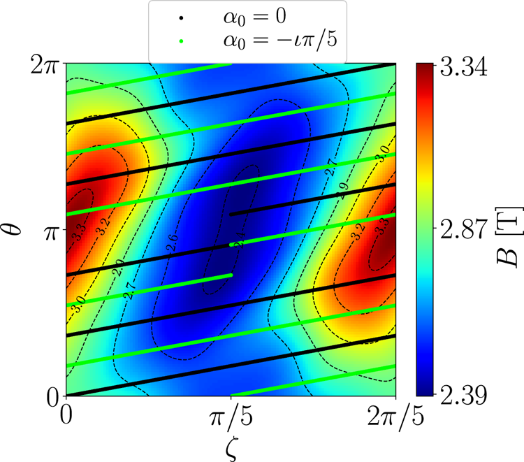The field line $\alpha _0=-\iota {\rm \pi}/5$ is centred with respect to the equatorial plane and the triangular toroidal plane $\zeta ={\rm \pi} /5$, hence the name triangular flux tube. A schematic view of these field lines for the flux surface $r_0/a=0.8$ is given in figure 1, where they are represented on a $(\theta,\zeta )$ plane with the magnetic field strength referred to the colour scale. 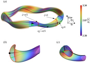A three-dimensional view of the surface $r_0/a=0.8$ is shown in figure 2(a) together with a sketch of our choice of flux coordinates and the field lines ${\alpha _0=0}$ and ${\alpha _0=-\iota {\rm \pi}/5}$. 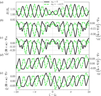Figures 2(b) and 2(c) show some details of figure 2(a). The geometric quantities required to solve equations (2.10) and (2.13) for the mentioned flux tubes are represented against the $\zeta$ coordinate, centred with respect to $\zeta _0=\zeta (\theta =0)$, in figure 3(a–e). In figure 3(a) it is observed that the magnetic field strength is symmetric with respect to $\zeta =\zeta _0$. This symmetry is also seen in the quantities $(\boldsymbol {\hat {b}}\times \boldsymbol {\nabla } B)\boldsymbol {\cdot } \boldsymbol {\nabla } \alpha$ and $(\boldsymbol {B}\times \boldsymbol {\kappa })\boldsymbol {\cdot } \boldsymbol {\nabla } \alpha$, which are represented in figures 3(b) and 3(c), respectively. In figures 3(d) and 3(e) we see that $(\boldsymbol {B}\times \boldsymbol {\kappa })\boldsymbol {\cdot }{\boldsymbol {\nabla } r}= (\boldsymbol {\hat {b}}\times \boldsymbol {\nabla } B)\boldsymbol {\cdot }{\boldsymbol {\nabla } r}$, as is the case for any ideal magnetohydrodynamic equilibria. In what follows, we will refer to the direction of $\boldsymbol {\nabla }\alpha$ as the binormal direction and to the direction of ${\boldsymbol {\nabla } r}$ as the radial direction. The description of the flux tubes is complete with the specification of their length, which has been defined as the number of turns in the poloidal direction, $N_{\theta }$. This length is chosen to correctly resolve the electrostatic potential $\hat {\varphi }_{\boldsymbol {k}_{\perp }}$ along the flux tube. Since the localization of the electrostatic potential varies with the wavenumber, different values of $N_{\theta }$ have been considered in each test. 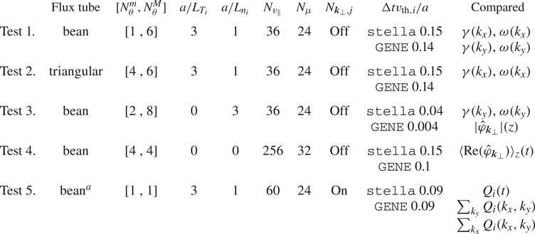The maximum and minimum values of $N_{\theta }$, $N_{\theta }^{M}$ and $N_{\theta }^{m}$, respectively, needed in each test are indicated in table 2, together with other parameters that define the simulations. These include the normalized ion temperature and density gradientsFootnote ³

(3.1)\begin{equation} {a/L_{T_i} :={-}a\left(\ln T_i\right)'}, \end{equation}

and

(3.2)\begin{equation} {a/L_{n_i} :={-}a\left(\ln n_i\right)'}, \end{equation}

the number of divisions in the velocity grid $(N_{v_{\|}},N_{\mu }$), the presence of nonlinear term ($N_{\boldsymbol {k}_{\perp },j}$), the time step size used for the calculation of the most unstable mode in each simulation and the different quantities compared in each test, where $\gamma$ refers to the growth rate, $\omega$ refers to the real frequency, $\langle \cdot \rangle _{z}$ means a line average and $Q_i$ is the ion heat flux. It is important to remark that we have always considered $128 \times N_{\theta }$ divisions in the grid of $z$. In addition, $Z_i=1$ and $T_i/T_e=1$ have been assumed. In what follows, the results of the tests are expressed in the coordinates $\{x,y,z\}$ used by stella, i.e. the ones defined in expressions (2.6) and (2.7) with $z = \zeta$.

Figure 1.

Schematic view of the magnetic field lines $\alpha _0=0$ (solid black line) and $\alpha _0=-\iota {\rm \pi}/5$ (solid green line) extended along the five field periods of W7-X. The magnetic field strength is represented in the background.

Figure 2.

Three-dimensional view of the surface $r_0/a=0.8$ (a), together with the field line $\alpha _0=0$ (solid black line), the field line $\alpha _0=-\iota {\rm \pi}/5$ (solid green line) and the last closed flux surface $r_0=a$ as a semi-transparent halo. Details of two toroidal cuts of the flux surface $r_0/a=0.8$ are also given, showing a bean-shaped section (b) and a triangular section (c).

Figure 3.

Normalized geometric quantities in the range $\zeta -\zeta _0=[-2{\rm \pi},2{\rm \pi} ]$ for the surface $r_0/a=0.8$ along the field lines $\alpha _0=0$ (solid black line) and $\alpha _0=-\iota {\rm \pi}/5$ (dashed green line). The magnetic field strength is represented in (a); the projections of $\boldsymbol {\hat {b}}\times \boldsymbol {\nabla } B$ and $\boldsymbol {B}\times \boldsymbol {\kappa }$ along the binormal direction are represented in (b,c), respectively; the projections of $\boldsymbol {\hat {b}}\times \boldsymbol {\nabla } B$ and $\boldsymbol {B}\times \boldsymbol {\kappa }$ along the radial direction are represented in (d,e), respectively.

Table 2.

Set of parameters used in each test. From left to right: flux tube, minimum and maximum number of $N_{\theta }$, normalized ion temperature and density gradients, number of divisions in the grid of $v_{\|}$ and $\mu$, presence of nonlinear term, time step size and quantities compared with both codes.

$^{a}$Nonlinear results obtained with stella in the triangular flux tube are also included in § 5.

4 Linear simulations

To perform a linear flux-tube gyrokinetic simulation, both codes solve the system of equations consisting of (2.10) and (2.13) dropping the nonlinear term of (2.10) and assuming $\hat {g}_{\boldsymbol {k}_{\perp }}$ and $\hat {\varphi }_{\boldsymbol {k}_{\perp }}$ to be proportional to $\exp [(\gamma -\mathrm {i} \omega )t]$, where $\gamma$ and $\omega$ are the growth rate and real frequency of each mode. In this section, four different linear tests are presented. In tests 1 and 2, ITGs are simulated. In test 3, density-gradient-driven TEMs are computed. Finally, the simulations of test 4 include the collisionless relaxation of a zonal electrostatic potential.

The linear properties of ITGs and TEMs in stellarators have been reported in a large number of studies by means of linear gyrokinetic simulations. Kornilov et al. (Reference Kornilov, Kleiber, Hatzky, Villard and Jost2004) studied the ITG structure and its stability in W7-X with the global particle-in-cell code Euterpe. This code has also been used to model the effects of radial electric fields on ITG modes for the geometries of W7-X and the Large Helical Device in Riemann, Kleiber & Borchardt (Reference Riemann, Kleiber and Borchardt2016). Xanthopoulos & Jenko (Reference Xanthopoulos and Jenko2007) and Proll, Xanthopoulos & Helander (Reference Proll, Xanthopoulos and Helander2013) used the code GENE to study the effect of changes in the density gradient and temperature ratio on ITGs and TEMs and to look at the stability properties of W7-X, comparing with other devices. GENE has also been used in Proll et al. (Reference Proll, Mynick, Xanthopoulos, Lazerson and Faber2015) to investigate how stellarators can be optimized with respect to TEMs and in Alcusón et al. (Reference Alcusón, Xanthopoulos, Plunk, Helander, Wilms, Turkin, von Stechow and Grulke2020) to analyse the growth rate of the instability as a function of the temperature and density scales for different configurations of W7-X. A theoretical study about the effects of ITGs and TEMs in non-axisymmetric devices, and particularly in W7-X, is summarized in Helander et al. (Reference Helander, Bird, Jenko, Kleiber, Plunk, Proll, Riemann and Xanthopoulos2015). Recently, in Sánchez et al. (Reference Sánchez, Garcıa-Regaña, Bañón Navarro, Proll, Mora Moreno, González-Jerez, Calvo, Kleiber, Riemann and Smoniewski2021), the codes Euterpe, GENE, stella and GENE-3D have been compared in order to assess the differences in the linear properties of ITGs and the zonal-flow relaxation that arise when different computational domains, namely, flux tube, full flux surface and radially global domain, are considered.

4.1 Test 1. Linear ITG simulations in the bean flux tube

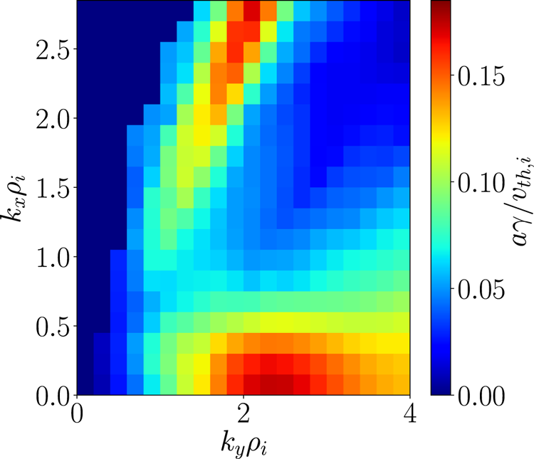
In this test, a linear ITG driven by a normalized ion temperature gradient $a/L_{T_i}=3$ with a normalized ion density gradient $a/L_{n_i}=1$ and adiabatic electrons is simulated in the bean flux tube (see table 2). In order to find the most unstable mode, a map containing the growth rate values as a function of the radial and binormal wavenumbers has been produced with stella and shown in figure 4. Note that the ion thermal Larmor gyroradius, $\rho _i$, is used for the normalization of wavevector components and it is defined as

(4.1)\begin{equation} \rho_i = \frac{v_{{\rm th},i}m_i}{Z_ieB_a}. \end{equation}

Two regions of large growth rate can be observed in this map. While $N_{\theta }=1$ is enough to simulate the region with $k_x\rho _i\lesssim 0.5$, $N_{\theta }=6$Footnote ⁴ is required to simulate the one including $k_x\rho _i\gtrsim 2$ due to the displacement in the $z$ direction of the parallel structure of the modes. The maximum growth rate found in this map is localized at $k_y\rho _i=2.1$. The codes GENE and stella have been used to compare the spectrum along $k_y$ for fixed $k_x$ and vice versa, capturing this wavenumber in both scans.

Figure 4.

ITG stability map corresponding to test 1. It shows the growth rate computed with the code stella in the bean flux tube as a function of $k_x$ and $k_y$.

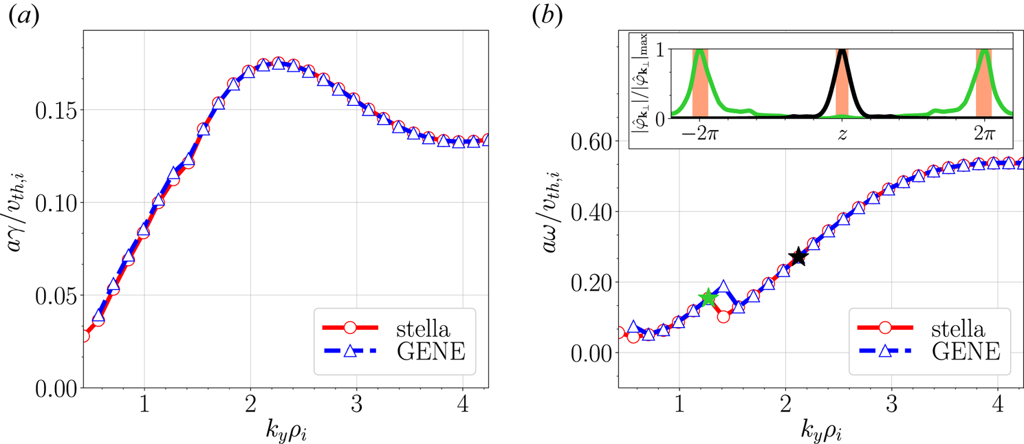
The comparison of growth rates and real frequencies as a function of $k_y$ for fixed $k_x=0$ is given in figures 5(a) and 5(b), respectively. These figures show an excellent agreement between stella and GENE. In figure 5(b) it is seen that the frequency is positive for every simulated mode. ITG-driven modes are expected to propagate in the ion diamagnetic direction, i.e. $\omega \omega _{*,i}>0$, where $\omega _{*,i}$ is the ion diamagnetic frequency, which, with our definitions and conventions, reads

(4.2)\begin{equation} {\omega_{*,i}={-}\mathrm{sgn}(\psi_{t,a})\frac{T_ik_y}{Z_ieB_aL_{n_i}}.} \end{equation}

As only positive values of $k_y$ are explored in this scan, $L_{n_i}>0$ (see table 2) and $\psi _{t,a}<0$ for the selected configuration (see the direction of $\boldsymbol {B}$ and the left-handed system sketched in figure 2a), we have $\omega _{*,i}>0$. This proves that, indeed, in this test $\omega \omega _{*,i}>0$, thus the studied ITG-driven modes propagate in the ion diamagnetic direction. A closer look at figure 5(b) shows a discontinuity in the frequency, which is associated with a change in the mode structure, defining two different branches of the ITG instability. This can be observed in the inset of figure 5(b), which represents, as a function of $z$, computations of stella for the modulus of the electrostatic potential normalized to its maximum value $(|\hat {\varphi }_{\boldsymbol {k}_{\perp }}|/|\hat {\varphi }_{\boldsymbol {k}_{\perp }}|_{\mathrm {max}})$ for the modes with $k_y\rho _i=\{1.3,2.1\}$. These modes are strongly localized in the highlighted red bands, which correspond to bad curvature regions, defined as those where

(4.3)\begin{equation} \frac{k_yT'_i}{\psi'_t}\left(\boldsymbol{\hat{b}}\times\boldsymbol{\nabla} B\right)\boldsymbol{\cdot}\boldsymbol{k}_{{\perp}}>0. \end{equation}

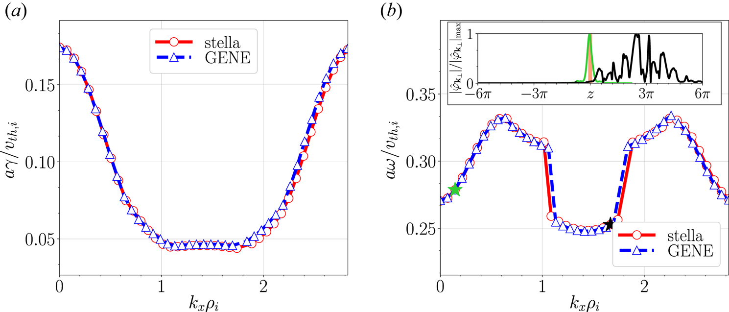
If $k_x=0$ and $k_y>0$, these regions are the ones where the quantity shown in figure 3(b) takes positive values. The growth rates and real frequencies as a function of $k_x$, keeping $k_y\rho _i=2.1$, can be seen in figures 6(a) and 6(b), respectively. As in the $k_y$-spectra, every mode studied in this scan propagates in the ion diamagnetic direction, as it can be observed in figure 6(b). This figure also shows a discontinuity in the frequency, giving rise to three different branches, located at $k_x\rho _i\in (0,1.0]$, $k_x\rho _i\in (1.0,1.8)$ and $k_x\rho _i\in [1.8,2.7)$. In the inset of figure 6(b), the structure of the modes with $k_x\rho _i=\{0.2,1.7\}$ computed with stella, belonging to the first and central branches, respectively, are represented as a function of $z$. As observed in this inset, the electrostatic potential associated with the first branch is strongly localized and $N_{\theta }=1$ has been sufficient to capture the parallel structure of this mode. On the other hand, the electrostatic potential associated with the central branch spreads along $z$, making it necessary to extend the flux-tube length up to $N_{\theta }=6$.

Figure 5.

Linear growth rate (a) and real frequency (b) as a function of $k_y$ obtained for the ITG scenario studied in test 1 using stella (open circles linked by a solid red line) and GENE (open triangles linked by a dashed blue line) in the bean flux tube. The inset of (b) shows the structure of the modes $(k_x\rho _i,k_y\rho _i)=(0,1.3)$ (green line) and $(k_x\rho _i, k_y\rho _i)=(0,2.1)$ (black line) together with some bad curvature regions (shaded in red).

Figure 6.

Linear growth rate (a) and real frequency (b) as a function of $k_x$ obtained for the ITG scenario studied in test 1 using stella (open circles linked by a solid red line) and GENE (open triangles linked by a dashed blue line) in the bean flux tube. The inset of figure (b) shows the structure of the modes $(k_x\rho _i,k_y\rho _i)=(0.2,2.1)$ (green line) and $(k_x\rho _i, k_y\rho _i)=(1.7,2.1)$ (black line), together with a bad curvature region (shaded in red).

4.2 Test 2. Linear ITG simulations in the triangular flux tube

In this test, a linear ITG instability driven by a normalized ion temperature gradient $a/L_{T_i}=3$ with a normalized ion density gradient $a/L_{n_i}=1$ and adiabatic electrons is simulated in the triangular flux tube (see table 2).

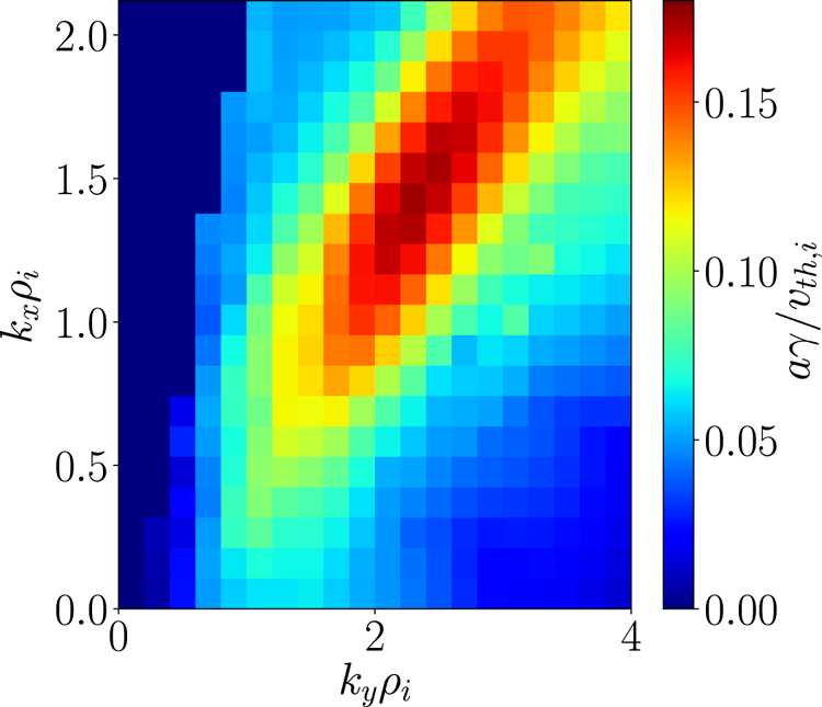
As in the previous test, in order to find the most unstable mode, a map of the growth rate for each pair $(k_x,k_y)$ has been produced with stella, see figure 7. As in the bean flux tube, the most unstable mode in this map is localized at $k_y\rho _i=2.1$. Interestingly, unlike in the bean flux tube, the maximum growth rate does not correspond to a mode with $k_x=0$. This figure also shows the triangular flux tube to be equally unstable as the bean one as $\gamma ^{\mathrm {max}}_{\mathrm {bean}}/\gamma ^{\mathrm {max}}_{\mathrm {triang}}\simeq 1$. The different localization in $k_x$ of the most unstable modes found in figures 4 and 7 implies that special care must be taken when comparing the linear stability properties of different flux tubes.

Figure 7.

ITG stability map corresponding to test 2. It shows the growth rate computed with the code stella in the triangular flux tube as a function of $k_x$ and $k_y$.

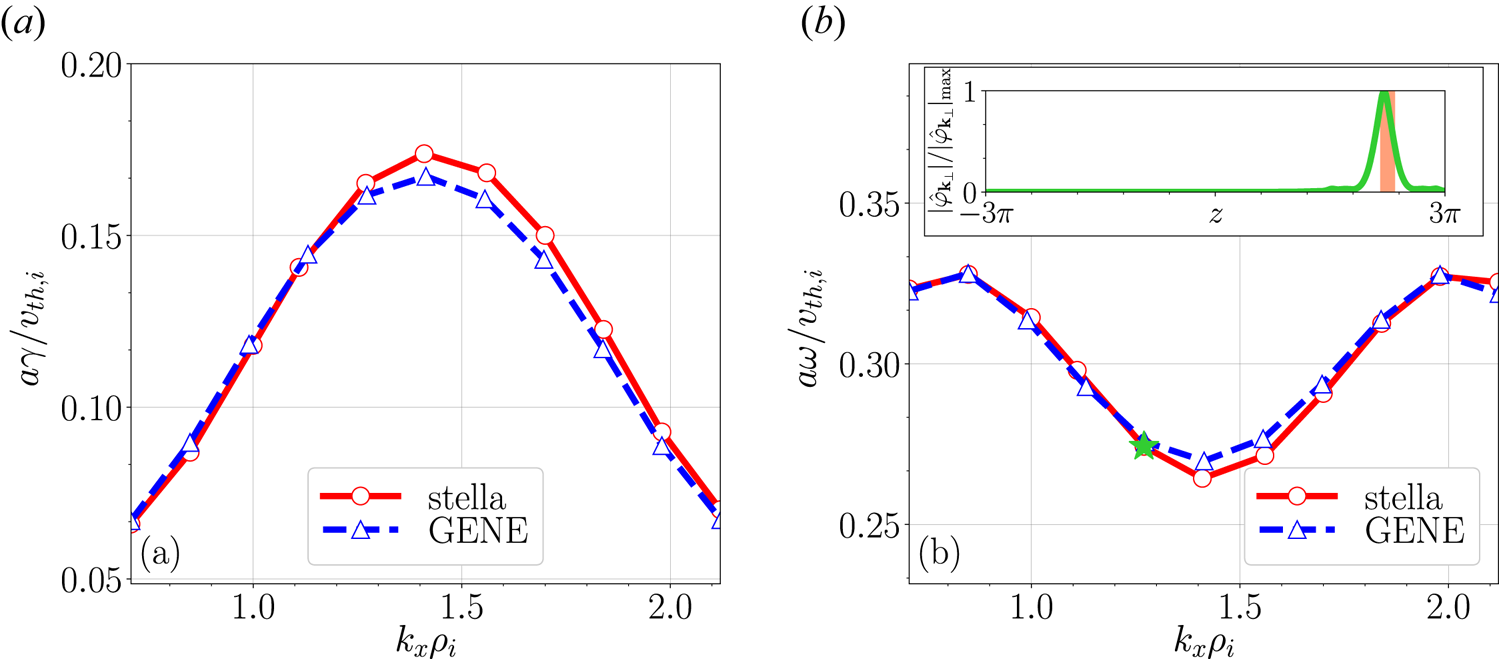
A scan along $k_x$, keeping $k_y\rho _i=2.1$, has been performed with both codes, representing the growth rates and real frequencies in figures 8(a) and 8(b), respectively. Although not as close as in the bean flux tube, the agreement between stella and GENE is still remarkable. As in the previous test, these modes propagate in the ion diamagnetic direction. In this scan, the localization of the electrostatic potential moves to higher values of $z$ when increasing $k_x$, making it necessary to extend the flux-tube length up to $N_{\theta }=6$. The inset of figure 8(b) includes the parallel structure of the mode with $k_x\rho _i=1.2$ obtained with stella, together with the bad curvature region where this mode is localized.

Figure 8.

Linear growth rate (a) and real frequency (b) as a function of $k_x$ obtained for the ITG scenario studied in test 2 using stella (open circles linked by a solid red line) and GENE (open triangles linked by a dashed blue line) in the triangular flux tube. The inset of figure (b) shows the structure of the mode $(k_x\rho _i,k_y\rho _i)=(1.2,2.1)$ (green line) together with a bad curvature region (shaded in red).

4.3 Test 3. Linear density-gradient-driven TEM simulations in the bean flux tube

In the third test, kinetic electrons are included. We study linear instabilities driven by normalized electron and ion density gradients $a/L_{n_e}=a/L_{n_i}=3$. In order to avoid the presence of temperature-gradient-driven modes, the electron and ion temperature gradients have been set to zero, $a/L_{T_e}=a/L_{T_i}=0$ (see table 2). We will refer to modes studied in this subsection as density-gradient-driven TEMs. 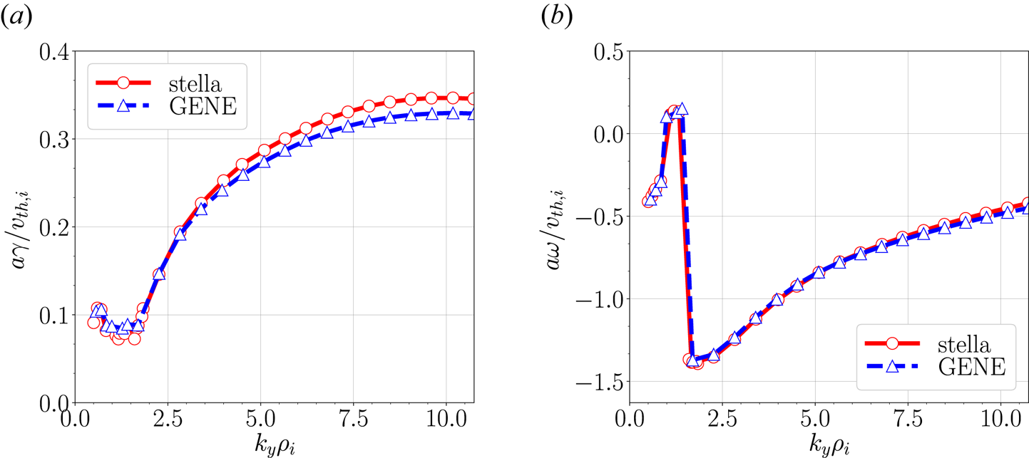It is worth noting (see $\Delta t v_{\mathrm {th},i}/a$ in table 2) how the mixed implicit–explicit method employed by stella allows a larger time step in these simulations than the explicit scheme used in GENE. This difference in the time step size results in a clear reduction of the total simulated time. In fact, while GENE has required 703 total CPU hours (5.49 h running in 128 processors) to complete the whole simulation, stella has needed 76 total CPU hours (0.53 h running in 144 processors) to simulate the same modes. 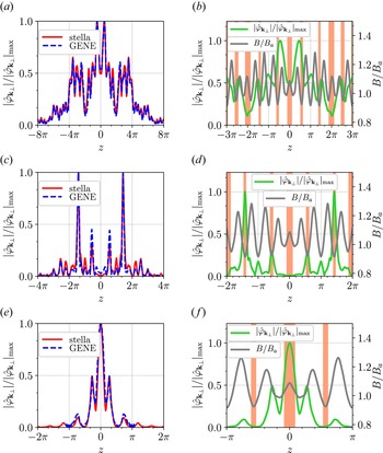The growth rate and real frequency values as a function of $k_y$, keeping $k_x=0$, are shown in figures 9(a) and 9(b), respectively. As observed in these figures, there is a remarkable agreement between the results obtained with stella and GENE. In figure 9(b) it can be seen that these modes can propagate both in the electronFootnote ⁵ and ion diamagnetic directions, depending on the wavenumber. A closer look at this figure allows us to clearly distinguish three different branches. The electrostatic potentials associated with the modes with $k_y\rho _i=\{{0.7},1.2,4.7\}$, each one belonging to a different branch, are represented as a function of $z$ for the whole length of the flux tube in figure 10(a,c,e), obtaining a good agreement between both codes. The same structures found in figure 10(a,c,e) are represented in figure 10(b,d,f), respectively, in a narrower $z$ range, together with the normalized magnetic field strength and the bad curvature regions. The parallel structure of the modes belonging to the first branch, in the range $k_y\rho _i=(0,1.1]$, has a particular shape (figure 10a,b), which can be identified with some structures discussed in Proll (Reference Proll2014). To resolve this electrostatic potential we have increased the flux-tube length up to $N_{\theta }=8$ with both codes. In order to study the second branch, in the narrow range of $k_y\rho _i=(1.0,1.5)$, the flux tube has been extended up to $N_{\theta }=4$. Finally, $N_{\theta }=2$ has been sufficient for the study of the third branch, covering from $k_y\rho _i=1.4$ to the end of the simulated range.

Figure 9.

Linear growth rate (a) and real frequency (b) as a function of $k_y$ obtained for the instabilities studied in test 3 using stella (open circles linked by a solid red line) and GENE (open triangles linked by a dashed blue line) in the bean flux tube.

Figure 10.

Normalized modulus of the electrostatic potential computed with stella (solid red line) and GENE (dashed blue line) as a function of $z$ over the entire length of the flux tube for some modes simulated in test 3; specifically, we are representing the modes $(k_x\rho _i, k_y\rho _i)= (0,{0.7})$ (a), $(0,1.2)$ (c) and $(0,4.7)$ (e). The structures calculated with stella are shown as solid green lines in narrower $z$ ranges in (b,d,f), respectively, together with the normalized magnetic field strength (grey line) and the bad curvature regions (shaded in red).

4.4 Test 4. Zonal-flow relaxation in the bean flux tube

Finally, we address the so-called Rosenbluth–Hinton test (Rosenbluth & Hinton Reference Rosenbluth and Hinton1998), which consists in the study of the linear collisionless time evolution of the zonal components of the potential, i.e. those with $k_y=0$, from their value at the initial time $t=0$ to their value when $t\rightarrow \infty$. The theoretical study of the zonal-flow response in stellarators has been addressed in Sugama & Watanabe (Reference Sugama and Watanabe2005), Mishchenko, Helander & Könies (Reference Mishchenko, Helander and Könies2008), Helander et al. (Reference Helander, Mishchenko, Kleiber and Xanthopoulos2011), Monreal et al. (Reference Monreal, Calvo, Sánchez, Parra, Bustos, Könies, Kleiber and Görler2016), Monreal et al. (Reference Monreal, Sánchez, Calvo, Bustos, Parra, Mishchenko, Könies and Kleiber2017) and Smoniewski et al. (Reference Smoniewski, Sánchez, Calvo, Pueschel and Talmadge2021). In non-axisymmetric devices, the relaxation of a zonal potential perturbation typically shows a damped oscillation, reaching a stationary residual level at $t\rightarrow \infty$. The damped oscillation involves two different frequencies with different time scales: the geodesic acoustic mode (GAM) oscillation (which is also found in tokamaks) and a low-frequency oscillation characteristic of the non-axisymmetric geometry of the stellarator. This characteristic low-frequency oscillation of the time evolution of the potential, only predicted for $k_x\rho _i\ll 1$ (Mishchenko et al. Reference Mishchenko, Helander and Könies2008; Helander et al. Reference Helander, Mishchenko, Kleiber and Xanthopoulos2011; Monreal et al. Reference Monreal, Sánchez, Calvo, Bustos, Parra, Mishchenko, Könies and Kleiber2017), has been experimentally identified in the TJ-II stellarator in Alonso et al. (Reference Alonso, Sánchez, Calvo, Velasco, McCarthy, Chmyga, Eliseev, Estrada, Kleiber and Krupnik2017).

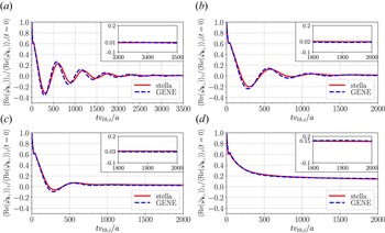
For simplicity, in the simulations included in this test $a/L_{T_i}=a/L_{n_i}=0$ have been considered. In addition, as initial condition we have imposed $\hat {\varphi }_{\boldsymbol {k}_{\perp }}(t=0)$ to be a Gaussian function centred in the middle of the flux tube. Four time traces of the line-averaged electrostatic potential normalized to its value at $t=0$ have been computed and represented in figure 11(a–d). In these panels, it can be observed how the results obtained with both codes for $k_x\rho _i\in \{0.05, 0.07, 0.1, 0.3\}$ match remarkably well. As already mentioned, the four time traces show an initial GAM oscillation at $tv_{{\rm th},i}/a<100$, followed, except for figure 11(d), by a lower-frequency damped oscillation. As observed in these figures, the frequency of the damped oscillation decreases with increasing $k_x$, in fact, for $k_x\rho _i=0.3$, represented in figure 11(d), this frequency is missing. The residual level of each time trace is given in the insets of these figures. These plots show that the residual value of the time traces increases with $k_x$.

Figure 11.

For test 4, time trace of the line-averaged electrostatic potential normalized to its maximum value computed with stella (solid red line) and with GENE (dashed blue line) for the pairs $(k_x\rho _i,k_y\rho _i)=(0.05,0)$ (a), $(k_x\rho _i,k_y\rho _i)=(0.07,0)$ (b), $(k_x\rho _i,k_y\rho _i)=(0.1,0)$ (c) and $(k_x\rho _i,k_y\rho _i)=(0.3,0)$ (d). The insets show a detail of each trace at large times.

5 Nonlinear simulations

In flux-tube nonlinear simulations, the codes solve (2.10) and (2.13) within a flux tube that extends in the radial and binormal directions. The parameters that define the flux tube for the nonlinear test presented in this section (test 5) are listed in table 3. The first nonlinear gyrokinetic simulations in W7-X were reported by Xanthopoulos et al. (Reference Xanthopoulos, Merz, Görler and Jenko2007), where GENE was used to study the nonlinear ITG-driven heat flux. Since then, GENE has been widely used to look at the nonlinear properties of turbulence in W7-X (Xanthopoulos et al. Reference Xanthopoulos, Mischchenko, Helander, Sugama and Watanabe2011; Helander et al. Reference Helander, Bird, Jenko, Kleiber, Plunk, Proll, Riemann and Xanthopoulos2015). More recently, in Bañón-Navarro et al. (Reference Bañón-Navarro, Merlo, Plunk, Xanthopoulos, von Stechow, Di Siena, Maurer, Hindenlang, Wilms and Jenko2020), the effects of ITG turbulent transport in different configurations of W7-X have been investigated with the global version of GENE, GENE-3D (Maurer et al. Reference Maurer, Bañón-Navarro, Dannert, Restelli, Hindenlang, Görler, Told, Jarema, Merlo and Jenko2020). In Sánchez et al. (Reference Sánchez, Mishchenko, García, Kleiber, Bottino and Villard2020) the ITG-driven heat flux has been studied using realistic plasma parameters with the global particle-in-cell gyrokinetic code Euterpe. Finally, simulations carried out with stella with all species treated kinetically have been employed to look at the transport of impurities driven by ITG and TEM turbulence in W7-X (Garcıa-Regaña et al. Reference Garcıa-Regaña, Barnes, Calvo, Parra, Alcusón, Davies, González-Jerez, Mollén, Sánchez and Velasco2021).

Table 3.

Parameters used by stella and GENE to define the flux tube in test 5. From left to right: normalized flux-tube size in the radial ($l_x$) and binormal ($l_y$) directions; number of modes in the radial ($N_{k_x}$) and binormal ($N_{k_y}$) directions; smallest positive wavenumber in the radial ($|k_{x}|_{\mathrm {min}}$) and binormal ($k_{y,\mathrm {min}}$) directions.

5.1 Test 5. Nonlinear ITG-driven heat flux

In this test, a nonlinear calculation of the ITG-driven heat flux is carried out considering adiabatic electrons. In addition, a normalized ion temperature gradient $a/L_{T_i}=3$ and a normalized ion density gradient $a/L_{n_i}=1$ are assumed (see tables 2 and 3 for the values of the simulation parameters). The heat fluxes presented in this test are defined by

(5.1)\begin{equation} Q_i = \left\langle\int\,{\rm d} ^{3} v \frac{m_iv^{2}}{2} \boldsymbol{v}_{E}\boldsymbol{\cdot} \boldsymbol{\nabla} r g_i\right\rangle, \end{equation}

where $\langle \cdot \rangle$ is the flux-surface average, $g_i$ is given by (2.8) and $\boldsymbol {v}_{E}$ is the turbulent $E\times B$ drift. In a flux tube, expression (5.1) takes the form

(5.2) \begin{gather} Q_i = \frac{{\rm \pi}\mathrm{sgn}(\psi_{t,a})}{B_a} \left(\int_{z_{\mathrm{min}}}^{z_{\mathrm{max}}}\frac{\,{\rm d} z}{\boldsymbol{B}\boldsymbol{\cdot}\boldsymbol{\nabla} z} \right)^{{-}1} \int^{z_{\mathrm{max}}}_{z{_{\mathrm{min}}}} \,{\rm d} z \int_{-\infty}^{\infty}\,{\rm d} v_{\|}\int_0^{\infty}\,{\rm d} \mu \left[\left(v_{\|}^{2} + \frac{2B\mu}{m_i}\right)\right. \nonumber\\ \left. \sum_{ k_{x}, k_{y} }\left( \mathrm{Im}\left(\hat{\varphi}_{\boldsymbol{k}_{{\perp}}}\hat{g}_{\boldsymbol{-k_{{\perp}}},i}\right)k_{y}{\rm J}_0({k_{{\perp}}}{v_{{\perp}}}/\varOmega_i)\right)\left(\boldsymbol{\hat{b}}\boldsymbol{\cdot}\boldsymbol{\nabla} z\right)^{{-}1} \right]. \end{gather}

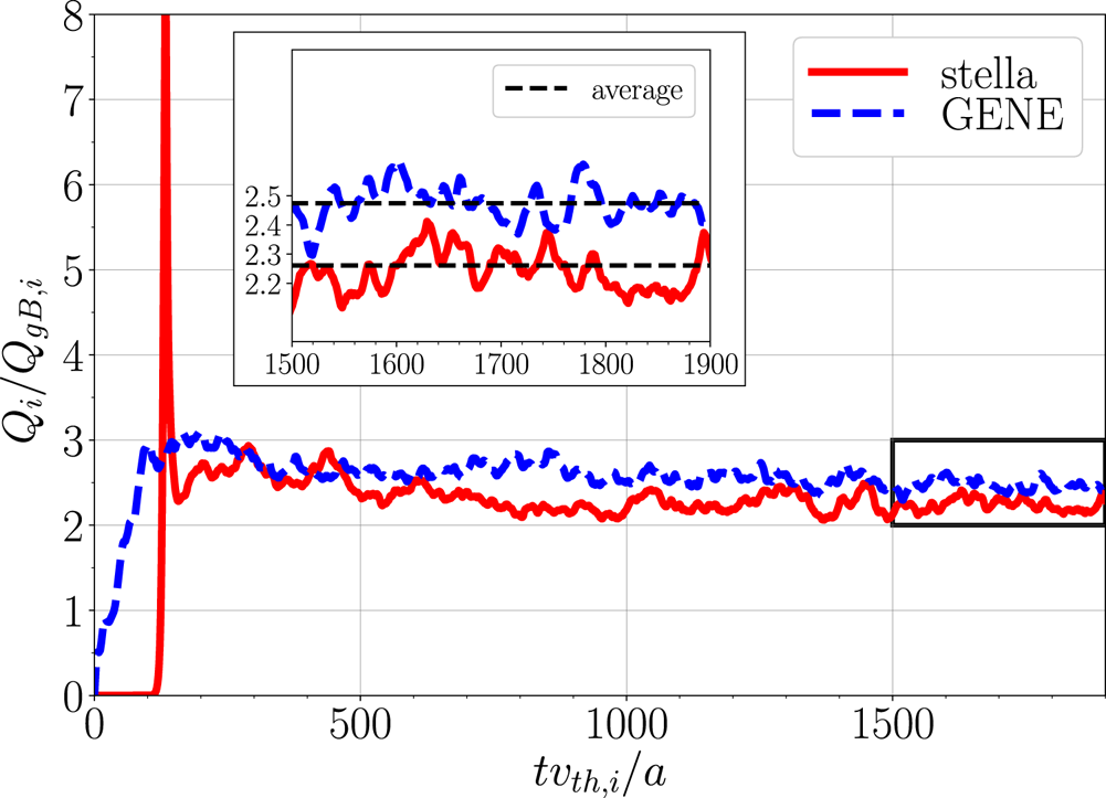
The time trace of the ITG-driven heat flux computed with both codes and normalized to the ion gyro-Bohm heat flux, $Q_{gB,i}=n_iT_iv_{{\rm th}{,i}}(\rho _i/a)^{2}$, is shown in figure 12. Despite the different initial evolution, both traces converge to very similar values. To quantify the difference between the saturated ITG-driven heat flux obtained with each code, an average over the time interval $tv_{{\rm th},i}/a=[1500, 1900]$ has been taken and represented in the inset of figure 12. The results for the normalized time-averaged ITG-driven heat flux computed with stella, which is $Q_i/Q_{gB,i}=2.26$ and GENE, which is $Q_i/Q_{gB,i}=2.47$, represent a difference around $8.5\,\%$. This slight difference may be caused by the different resolution in the flux tube used by each code, see table 3.

Figure 12.

Time trace of the normalized ITG-driven heat flux computed with stella (solid red line) and GENE (dashed blue line) in the bean flux tube for the test 5 ITG scenario. The inset shows a detail of the time interval $tv_{{\rm th},i}/a=[1500, 1900]$, with the heat flux time average given by the black dashed lines.

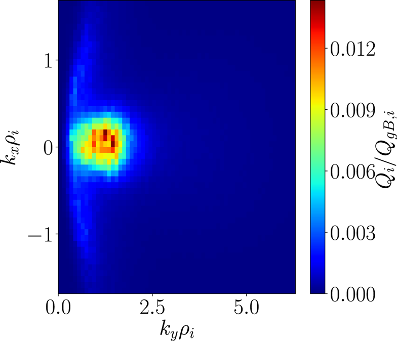
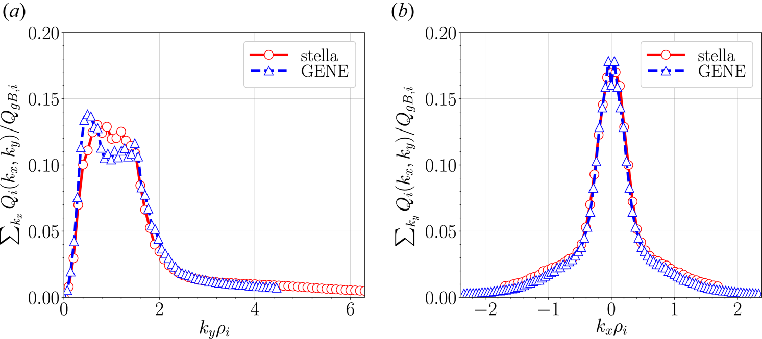
In order to provide a more comprehensive study of these results, stella has been used to compute the contribution of each pair $(k_x,k_y)$ to the time-averaged ITG-driven heat flux. In figure 13, it can be observed that the modes which contribute the most to the heat flux are those with $k_y\rho _i\lesssim 2.0$ and $|k_x\rho _i|\lesssim 0.5$. To compare these results with GENE calculations, the time-averaged ITG-driven heat flux is represented as a function of $k_y$, summing over $k_x$, in figure 14(a), and as function of $k_x$, summing over $k_y$, in figure 14(b). These figures show a satisfactory agreement between both codes.

Figure 13.

Normalized nonlinear ITG-driven heat flux computed with stella in the bean flux tube, averaged over the time interval $tv_{{\rm th},i}/a=[1500, 1900]$ and represented as a function of $k_x$ and $k_y$.

Figure 14.

Normalized ITG-driven heat flux averaged over the time interval $tv_{{\rm th},i}/a=[1500, 1900]$ computed with stella (open circles linked by a solid red line) and GENE (open triangles linked by a dashed blue line) in the bean flux tube. It is represented as a function of $k_y$, summing over $k_x$ (a) and as a function of $k_x$, summing over $k_y$ (b).

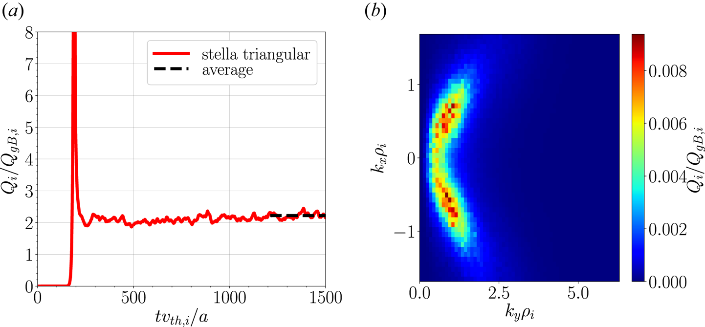
Finally, for the sake of completeness, a simulation in the triangular flux tube performed with stella has been included in this section. The parameters selected to carry this simulation out are the ones collected in tables 2 and 3 for test 5. The time trace of the normalized ITG-driven heat flux and the contribution of each mode are represented in figures 15(a) and 15(b), respectively. Figure 15(a) shows the saturated ITG-driven heat flux in the triangular flux tube to be $Q_i/Q_{gB,i}=2.22$. This value is very similar to the one obtained in the bean flux tube using stella. The main differences between nonlinear ITG-driven heat flux calculations in both flux tubes are found in their spectrum, as can be seen by comparing the maps given in figures 13 and 15(b). As in the bean flux tube, the modes in the binormal direction which contribute the most to the total heat flux in the triangular flux tube are those with $k_y\rho _i\lesssim 2.0$. However, in contrast with the results obtained for the bean flux tube, modes in the radial direction with $0.5\lesssim |k_x\rho _i|\lesssim 1.5$ make a large contribution to the total heat flux in the triangular flux tube.

Figure 15.

Time trace of the normalized ITG-driven heat flux computed with stella in the triangular flux tube, together with the heat flux time average over $tv_{{\rm th},i}/a=[1200,1500]$, represented with a black dashed line (a). This time-averaged ITG-driven heat flux is also represented as a function of $k_x$ and $k_y$ (b).

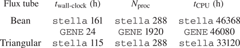
For a complete view of these nonlinear simulations, we have indicated in table 4 the simulation wall-clock time ($t_{\text {wall-clock}}$) required to produce these results. This table also includes the number of processors ($N_{\mathrm {proc}}$) on which the codes have been running and the total CPU time ($t_{\mathrm {CPU}}$) that each simulation has taken, defined as $t_{\mathrm {CPU}} = N_{\mathrm {proc}}\times t_{\text {wall-clock}}$. As expected, since we have assumed adiabatic electrons in these nonlinear calculations, both codes require similar $t_{\mathrm {CPU}}$ to perform the presented nonlinear test, as is shown in table 4. On the other hand, the time difference when simulating the triangular and bean flux tubes with stella is attributable to the different time ranges explored with each simulation, see figures 12 and 15(left).

Table 4.

Time required to run the nonlinear simulations with GENE in the bean flux tube and with stella in the bean and triangular flux tubes. From left to right: simulation wall-clock time in hours, number of processors and total CPU time in hours.

6 Summary and conclusions

Due to the increasing interest in stellarator gyrokinetic modelling, fostered by the results of W7-X first experimental campaigns, it is desirable to have a sufficiently complete, documented and well-verified set of linear and nonlinear gyrokinetic simulations in W7-X geometry against which present and future stellarator gyrokinetic codes can be tested and benchmarked. In this paper, such a set of simulations has been provided in the form of a comprehensive benchmark between the codes stella and GENE. This benchmark, consisting of five different tests, has been carried out in a fixed-boundary high-mirror configuration of W7-X. The linear part of the benchmark has been presented in tests 1 to 4. ITG instabilities have been studied in the bean and triangular flux tubes of W7-X in tests 1 and 2, respectively. Comparing these results, it can be concluded that both flux tubes are equally unstable, but the largest growth rates are found at different radial wavenumbers. TEM instabilities driven by density gradients have been studied in test 3, where it has been shown how the mixed implicit–explicit method used by stella allows us to use larger time steps than explicit codes for simulations with kinetic electrons, resulting in a clear reduction of the total CPU time. In these three tests, the structure of the electrostatic potential associated with each instability has been given and the growth rate and real frequency values obtained with stella and GENE have been successfully compared. In test 4, different time traces of the zonal electrostatic potential relaxation have been compared. Finally, the nonlinear ITG-driven heat flux and its spectrum have been calculated in test 5 in the bean flux tube with both codes and, for completeness, in the triangular flux tube with stella. The computed energy fluxes are similar in both flux tubes, although the radial modes that make the largest contribution to the total heat flux are different.