


1. Introduction and main results
In early February 2025, Professor Mahendra Panthee delivered a talk about his work with Bona et al. [Reference Bona, Chen, Hong, Panthee and Scialom2] on long wavelength limit of the BBM equation. While I was watching his interesting talk, I started wondering whether those ideas could be extended to more general models.
My main motivation for this work was the fact that the model considered by Panthee in his talk was, to a certain extent, a dynamical system in a Banach space, which in some sense is an example illustrating why the study of solutions of systems of ODEs like
 \begin{equation*}
\left\{
\begin{array}{lcl}
u'(t) &=&f(t,u), \\
\\
u(0)&=&u_0,
\end{array}
\right.
\end{equation*}
where  $u=(u^1,\cdots,u^n)\in\mathbb{R}^n$ and
 $f$ is a continuous function, is not only a classical problem, dating back to the origins of differential calculus, but it is still a topic of interest [Reference Constantin5, Reference Constantin6].
The works by Peano [Reference Peano11, Reference Peano12] shed light on the problem of existence and uniqueness of solutions of such a problem in  $\mathbb{R}^n$. The main tool for such a result is the beautiful, simple, but powerful Fixed Point Theorem for contractions.
Peano’s ideas have been generalized and applied to more abstract and general dynamical systems than in  $\mathbb{R}^n$. A significant part of qualitative studies of models with time evolution is currently carried out by replacing the curve
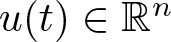 $u(t)\in\mathbb{R}^n$,
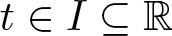 $t\in I\subseteq\mathbb{R}$, by objects evolving in other Banach spaces, where the initial datum, that is, a point in the system above, is now seen as a function. As such, currently, we can treat certain partial differential equations (PDEs) as ODEs. This observation, in particular, is true for many equations with relevance in hydrodynamics, as is the case with the BBM equation.
We now fix the language used throughout the paper and then state our main results.
1.1. Notation
The symbols  $\mathcal{B}$ and
 $A$ denote, respectively, a generic Banach space and a subset of the real line. For us,
 $A$ will be either the real line
 $\mathbb{R}$ or
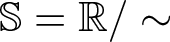 $\mathbb{S}=\mathbb{R}/\sim$, where
 $a\sim b$ if and only if
 $b-a\in\mathbb{Z}$. By
 $\mathbb{N}$, we mean the set of positive integer numbers.
By  $|x|$ we either mean the absolute value of a scalar
 $x$, or the sum
 \begin{equation*}|x|:=|x_1|+\cdots+|x_n|\end{equation*}
in case  $x=(x_1,\cdots,x_n)$ is a vector.
Very often, the Banach space  $\mathcal{B}$ is regarded as a product space, that is
 $\mathcal{B}=\mathcal{B}_1\times\cdots\times\mathcal{B}_n$, where
 $\mathcal{B}_i$,
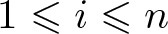 $1\leqslant i\leqslant n$, are Banach spaces as well. In this way, a member
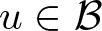 $u\in\mathcal{B}$ is a vector
 $u=(u^1,\cdots,u^n)$, where
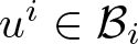 $u^i\in\mathcal{B}_i$.
Let  $T_k:\mathcal{B}\rightarrow \mathcal{B}$ be an integral operator with kernel
 $k$, that is,
 \begin{equation*}
(T_k(\psi))(x)=\int_A k(x,y)\psi(y)dy.
\end{equation*}
In case  $\mathcal{B}$ is a product space and
 $\psi=(\psi^1,\cdots,\psi^n)\in \mathcal{B}$, then the above equality has to be understood as
 \begin{equation}
(T_k(\psi))(x)=\Big(\int_A k_1(x,y)\psi^1(y)dy, \cdots,\int_A k_n(x,y)\psi^n(y)dy\Big)
\end{equation}
with
 \begin{equation*}
k(x,y)=(k_1(x,y),\cdots,k_n(x,y)),
\end{equation*}
where 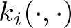 $k_i(\cdot,\cdot)$,
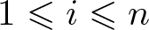 $1\leqslant i\leqslant n$, are functions for which the integrals are well defined or tempered distributions.
Remark 1.1. There is somewhat a sort of abuse of notation and definition concerning (1.1). In the case of tempered distribution, the integrals in (1.1) involving kernels 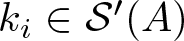 $k_i\in{\mathcal S}'(A)$ are understood in the sense of tempered distributions, i.e., via duality—or pairing—with test functions.
Let 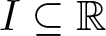 $I\subseteq{\mathbb{R}}$ be an interval. By
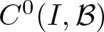 $C^0(I,\mathcal{B})$ we denote the set of bounded continuous functions
 $I\ni t\mapsto u(t,\cdot)\in \mathcal{B}$. This space is endowed with the norm
 \begin{equation}
\|u\|:=\sup_{t\in I}\|u(t,\cdot)\|_{\mathcal{B}}.
\end{equation}
For a function  $v:A\rightarrow\mathbb{R}$, we have
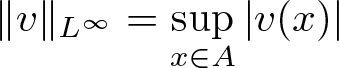 $\|v\|_{L^\infty}=\sup\limits_{x\in A}|v(x)|$.
1.2. Main results
We recall a rather useful definition for our purposes.
Definition 1.2. A function 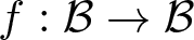 $f:\mathcal{B}\rightarrow\mathcal{B}$ is said to be locally Lipschitz if, for every
 $r \gt 0$, there exists
 $M{=M(r)} \gt 0$ such that
 \begin{equation*}\|f(x)-f(y)\|_{\mathcal{B}}\leqslant M\|x-y\|_{\mathcal{B}}\end{equation*}
provide that  $\|x-y\|_{\mathcal{B}}\leqslant r$. If the conditions above hold for the same
 $M$, for any
 $r \gt 0$, then
 $f$ is said to be (globally) Lipschitz.
Typical locally Lipschitz functions are those continuously differentiable  $f:\mathbb{R}^n\rightarrow\mathbb{R}^n$.
Let us denote  $f(x)=(f^1(x),\cdots,f^n(x))$ and some closed ball
 $B$ of radius
 $r \gt 0$ in
 $\mathbb{R}^n$. By the mean value inequality, we have
 \begin{equation*}|f^i(x)-f^i(y)|\leqslant \max_{t\in[0,1]}\max_{x,y\in B}\Big|\frac{d}{dt}f^i(ty+(1-t)x)\Big||x-y|=:M_i|x-y|,\end{equation*}
meaning that
 \begin{equation*}|f(x)-f(y)|\leqslant M|x-y|,\end{equation*}
for some positive constant  $M$.
Henceforth,  $a$ denotes a locally Lipschitz function, that is, for some
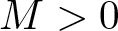 $M \gt 0$,
 \begin{equation}
| a(u)-a(v)|\leqslant M|u-v|,
\end{equation}
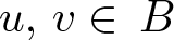
provided that  $u$ and
 $v$ are within the same ball in
 $\mathcal{B}$.
Consider the Cauchy problem
 \begin{equation}
\left\{
\begin{array}{lcl}
\displaystyle{\frac{d}{dt}u(t,x)}&=&T_k(a(u))(t,x),\\
\\
u(0,x)&=&u_0(x),
\end{array}
\right.
\end{equation}
where the right-hand side of the equation in (1.4) is given by
 \begin{equation}
T_k(a(u))(t,x)=\int_A k(x,y)a(u(t,y))dy,
\end{equation}
and the expression above must be understood in the sense already mentioned in (1.1).
The main result of this paper is the following:
Theorem 1.3. Let 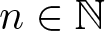 $n\in\mathbb{N}$,
 $k=(k_1,\ldots,k_n)$, such that are
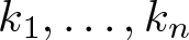 $k_1,\ldots,k_n$ tempered distributions (see Remark 1.1) and
 \begin{equation}
c_1:=\sup_{x\in A}\int_A \Big|k(x,y)\Big|dy \lt \infty;
\end{equation}
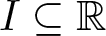 $I\subseteq\mathbb{R}$ an interval,
 $\mathcal{B}$ a Banach space of functions
 $u:I\times A\rightarrow\mathbb{R}^n$,
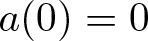
 $a:\mathbb{R}^n\rightarrow \mathbb{R}^n$ be a locally Lipschitz function, with
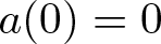 $a(0)=0$, satisfying (1.3),
 $T_k:\mathcal{B}\rightarrow \mathcal{B}$ be a continuous operator given by (1.5).
Then there exists a value 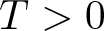 $T \gt 0$, depending on
 $c_1$ and
 $|a|_{L^\infty}$, such that the Cauchy problem (1.4) has a unique local solution
 $u\in C^0([0,T];\mathcal{B})$.
Additionally, if, for some positive and continuous function 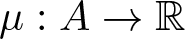 $\mu:A\rightarrow\mathbb{R}$, such that
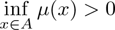 $\inf\limits_{x\in A}\mu(x) \gt 0$ and
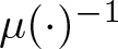 $\mu(\cdot)^{-1}$ is a locally integrable function, we have
 \begin{equation}
M\sup_{x\in A}\Big(\mu(x)\int_A\frac{|k(x,y)|}{\mu(y)}dy\Big)\leqslant c_0 \lt \infty,
\end{equation}
for some positive constant  $c_0$, and given an initial datum
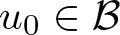 $u_0\in\mathcal{B}$ we have another constant
 \begin{equation}
\gamma:=\sup_{x\in A}\Big(|u_0(x)|\mu(x)\Big) \lt \infty,
\end{equation}
then the corresponding solution of (1.4) inherits the condition (1.8), that is
 \begin{equation}
\sup_{x\in A}\Big(|u(t,x)|\mu(x)\Big)\leqslant\gamma e^{c_0t}.
\end{equation}
Remark 1.4. The conditions on  $\mu$ imply that the integral in (1.7) is well-defined. Moreover, since its inverse
 $\mu^{-1}$ is integrable, whenever
 $A=\mathbb{R}$, then
 \begin{equation*}\lim_{|x|\rightarrow\infty}\frac{1}{\mu(x)}=0,\end{equation*}
provided that  $\mu$ is not constant outside some compact set, meaning that
 $\mu$ may not be bounded. Therefore, if the initial datum satisfies (1.8), then
 $u$ decays at least
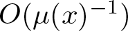 $O(\mu(x)^{-1})$ as
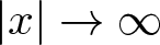 $|x|\rightarrow\infty$, for each fixed
 $t$ for which the solution exists.
Remark 1.5. Condition (1.7) is always satisfied if one considers the Dirac delta distribution as the kernel of (1.5). One may ask, however, the meaning of (1.6) when  $k(x,y)=\delta(x-y)$. We have two possibilities: the easiest one is only taking
 $|\delta(x)|=\delta(x)$. A more rigorous way to address the point would be taking a family of functions
 $\delta_\epsilon$ convergent (in the weak sense) to
 $\delta$ as
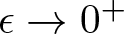 $\epsilon\rightarrow0^+$. Such a family can be chosen as being non-negative, so that
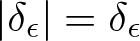 $|\delta_\epsilon|=\delta_\epsilon$. In this way, we would then conclude that
 $|\delta(x)|=\delta(x)$. An example of a family of functions having such a property is precisely the heat kernel.
In the next two results, we use Theorem 1.3 to derive asymptotic bounds for solutions of PDEs as long as they exist in time. These solutions are considered in the Sobolev spaces 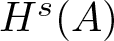 $H^s(A)$, for some
 $s\in\mathbb{R}$. For definitions and details about Sobolev spaces, see [Reference Taylor13, Chapter 4]. Moreover, whenever
 $A=\mathbb{S}$, we must bear in mind the addition of the periodic condition
 $v(x+1)=v(x)$ in all the involved functions in the variable
 $x$.
Henceforth, we use the following distributions:
 \begin{equation}
g(x)=\left\{
\begin{array}{ll}
\displaystyle{\frac{e^{-|x|}}{2}},&\text{if}\,\,A=\mathbb{R},\\
\\
\displaystyle{\frac{\cosh(x-\lfloor x \rfloor - 1/2)}{2\sinh(1/2)}}, & \text{if}\,\,A=\mathbb{S},
\end{array}
\right.
\end{equation}
whose corresponding distributional derivatives are:
 \begin{equation*}
\partial_xg(x)=\left\{
\begin{array}{ll}
\displaystyle{-\text{sgn}{(x)}\,\frac{e^{-|x|}}{2}},&\text{if}\,\,A=\mathbb{R},\\
\\
\displaystyle{\frac{\sinh(x-\lfloor x \rfloor - 1/2)}{2\sinh(1/2)}}, & \text{if}\,\,A=\mathbb{S}.
\end{array}
\right.
\end{equation*}
Remark 1.6. Condition (1.7) encloses a subtle fact: due to condition (1.6), one might expect (1.7) being satisfied for functions  $\mu$ with a strong growth. This is not necessarily true in general.
For example, consider  $A=\mathbb{R}$, take
 $k(x,y)=g(x-y)$ and
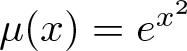 $\mu(x)=e^{x^2}$, where
 $g$ is given by (1.10). Then we have
 \begin{align}
h(x)&:=\int_{\mathbb{R}} \frac{g(x-y)}{\mu(y)}dy=\int_{\mathbb{R}} e^{-|x-y|-y^2}dy \nonumber\\
&=\frac{\sqrt{\pi}}{4}e^{\frac{1}{4}}\Big(e^{-x}\texttt{Erfc}\Big(\frac{1}{2}-x\Big)+e^{x}\texttt{Erfc}\Big(\frac{1}{2}+x\Big)\Big),
\end{align}
where  $\texttt{Erfc}$ is the complementary error function, given by
 \begin{equation*}
\texttt{Erfc}(x)=1-\frac{2}{\sqrt{\pi}}\int_0^xe^{-z^2}dz.
\end{equation*}
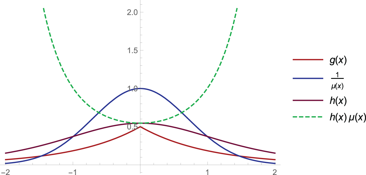
Therefore, (1.7) cannot be satisfied. See Figure 1.
Graphs of the functions discussed in Remark 1.6. Above  $g(x)=e^{-|x|}/2$,
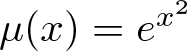 $\mu(x)=e^{x^2}$ and
 $h$ is given in (1.11). Both
 $g$ and
 $\mu^{-1}$ have a strong decay at infinity, as well as the result of their convolution, that is the function
 $h$ above. The behaviour of
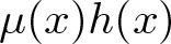 $\mu(x)h(x)$ (in dashed green), however, is rather different from the others, showing an unbounded function.

Theorem 1.7. Let  $a:\mathbb{R}^n\rightarrow\mathbb{R}^n$ be a continuously differentiable function, with bounded derivative and
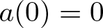 $a(0)=0$,
 $u_0\in H^s(A)$,
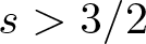 $s \gt 3/2$, and consider the Cauchy problem
 \begin{equation}
\left\{
\begin{array}{lcl}
u_{t}&=&((\partial_xg)\ast a(u)),\\
\\
u(0,x)&=&u_0(x).
\end{array}
\right.
\end{equation}
Then (1.12) has a unique local solution  $u\in C^0([0,T];H^s(A))$, for some
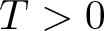 $T \gt 0$. Moreover, if
 \begin{equation}
\sup_{x\in A}\Big(e^{b|x|}|u_0(x)|\Big) \lt \infty,
\end{equation}
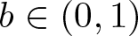 $b\in(0,1)$, then there exist positive constants
 $c_0$ and
 $\gamma$ such that
 \begin{equation}
|u(t,x)|\leqslant\gamma e^{c_0t-b|x|}.
\end{equation}
In particular, if  $A=\mathbb{S}$, we have
 \begin{equation}
|u(t,x)|\leqslant \gamma e^{c_0t-b|x-\lfloor x \rfloor|},
\end{equation}
for any 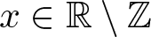 $x\in\mathbb{R}\setminus\mathbb{Z}$, where
 $\lfloor x \rfloor$ denotes the greatest integer part of
 $x$.
Theorem 1.8. Assume that  $u_0,\,u_1\in H^s(\mathbb{R})\cap L^\infty(\mathbb{R})$,
 $s\geqslant 0$,
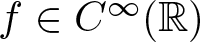 $f\in C^\infty(\mathbb{R})$, with
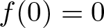 $f(0)=0$. Then the problem
 \begin{equation}
\left\{
\begin{array}{lcl}
u_{tt}&=&\partial_x^2 f(u)+u_{ttxx},\\
\\
u(0,x)&=&u_0(x),\\
\\
u_t(0,x)&=&u_1(x)
\end{array}
\right.
\end{equation}
has a unique solution  $u\in C^2([0,T];H^s(\mathbb{R})\cap L^\infty(\mathbb{R}))$. Moreover, assume that
 \begin{equation}
\sup_{x\in\mathbb{R}}\Big[e^{b|x|}\Big(|u_0(x)|+|u_1(x)|\Big)\Big] \lt \infty,
\end{equation}
for some 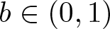 $b\in(0,1)$. Then there exist a closed ball of radius
 $r \gt 0$,
 $B=\{u\in H^s(\mathbb{R});\,\, \|u-u_0\|_{H^s(\mathbb{R})}+\|u_t-u_1\|_{H^s(\mathbb{R})}\leqslant r\}$ and two positive constants
 $c_0$ and
 $\gamma$ such that the corresponding solution emanating from (1.15) and its time derivative
 $u_t$ satisfy
 \begin{equation}
|u(t,x)|+|u_t(t,x)|\leqslant\gamma e^{c_0t-b|x|},
\end{equation}
where
 \begin{equation}
c_0= \frac{3-2b^2}{1-b^2}\Big(1+\sup_{|z|\leqslant r}|f'(z)|\Big).
\end{equation}
1.3. Novelty of the manuscript
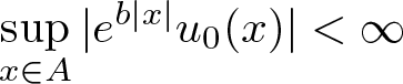
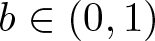
• We extend the qualitative results reported in [Reference Bona, Chen, Hong, Panthee and Scialom2] for solutions subject initial data satisfying general decaying rates. While in [Reference Bona, Chen, Hong, Panthee and Scialom2] the authors considered initial conditions satisfying
 $\sup\limits_{x\in A}|e^{b|x|}u_0(x)| \lt \infty$, where
$b\in(0,1)$ and
$A$ is either
$\mathbb{R}$ or
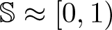
$\mathbb{S}\approx[0,1)$, in the present manuscript we establish our results assuming
for some general function
\begin{equation*}\sup\limits_{x\in A}|\mu(x)u_0(x)| \lt \infty,\end{equation*}
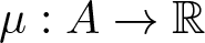
$\mu:A\rightarrow\mathbb{R}$, such that
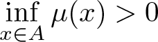
$\inf\limits_{x\in A}\mu(x) \gt 0$ and
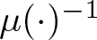
$\mu(\cdot)^{-1}$ is integrable.
• Beyond the above-mentioned extension, we generalize the ideas in [Reference Bona, Chen, Hong, Panthee and Scialom2] from the scalar BBM equation to an abstract ODE in a Banach space.
• In consequence of our general results, we proved persistence properties for the BBM-type system derived in [Reference Bona and Chen3] as a two-dimensional model describing propagation of waves in channels.
• We also established persistence properties for a generalized Boussinesq equation that encloses models describing waves in weakly dispersive media and non-linear Alfvén waves, see [Reference Clarkson, LeVeque and Saxton4, Reference Makhankov10, Reference Turitsyn14]. As far as the author knows, no result concerning persistence properties of the solutions have not been previously considered.



1.4. Structure of the paper
The outline of the paper is as follows: in the next section, we prove Theorem 1.3. In Section 3, we apply it to study classical ODE problems in  $\mathbb{R}^n$ and discuss problems related to grow-up of solutions and our exponential growth limitation. In Section 4, we prove Theorem 1.7 and apply it to some models. We also discuss some of the results obtained in [Reference Bona, Chen, Hong, Panthee and Scialom2] in light of the ones we are reporting here. In Section 5, we prove Theorem 1.8, which essentially establishes persistence properties for the generalized Boussinesq equation considered by Constantin and Molinet in [Reference Constantin and Molinet7].
2. Proof of Theorem 1.3
Let us first prove the existence and uniqueness of solutions for (1.4) in 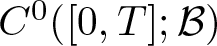 $C^0([0,T];\mathcal{B})$, for some
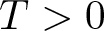 $T \gt 0$. Our strategy is the following: given a closed ball
 $B$ in
 $\mathcal{B}$, we estimate a value
 $T$ that will be used to prove the existence and uniqueness of a local solution in
 $C^0([0,T];B)\subseteq C^0([0,T];\mathcal{B})$. Finally, we prove (1.9).
• Ball and an interval for the existence of solution.
Let
$a$,
$T_k$,
$u_0$,
$r \gt 0$ and
$B=\{u\in \mathcal{B};\,\,\|u-u_0\|_{L^\infty}\leqslant r\}$ and
\begin{equation*}R:=r+\|u_0\|_{L^\infty}.\end{equation*}Condition
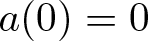
$a(0)=0$ combined with (1.3) tell us that
\begin{equation*}\sup_{|z|\leqslant R}|a(z)|\leqslant M(r+\|u_0\|_{L^\infty})=:L.\end{equation*}For now, let us formally define
(2.1)\begin{equation}
(Fu)(t,x)=u_0(x)+\int_0^t\Big(\int_A k(x,y)a(u(\tau,y))dy\Big)d\tau.
\end{equation}For
$u\in B$ and using (1.6), we have
(2.2)\begin{align}
|(Fu)(t,x)-u_0(x)|&\leqslant \int_0^t\int_A|k(x,y)||a(u(\tau,y))|dyd\tau \nonumber\\
&\leqslant \int_0^t\int_A|k(x,y)|\sup\limits_{|z|\leqslant R}|a(z)|dyd\tau\leqslant c_1Lt.
\end{align}Therefore, as long as
(2.3)we have\begin{equation}
t\leqslant \frac{r}{c_1L}\leqslant { T}\leqslant\frac{1}{c_1M}
\end{equation}
$(Fu)(t,\cdot)\in B$. As a consequence of our hypothesis, (2.1) defines a map
$F:C^0([0,T],B)\rightarrow C^0([0,T],B)$.• Existence and uniqueness of a local solution.
If (1.6) and (1.3) hold, then, for any
$u,\,v\in\,B$, and taking into account (1.2), we have
\begin{align*}
|(Fu)(t,x)-(Fv)(t,x)|&\leqslant \int_0^t\int_A|k(x,y)||a(u(\tau,y))-a(v(\tau,y))|dy d\tau \nonumber\\
&\leqslant c_1tM\|u-v\|.
\end{align*}Let us now proceed in a similar way, but now replacing
$u$ and
$v$ by
$(Fu)$ and
$(Fv)$. A similar calculation shows that
\begin{equation*}
|(F^2u)(t,x)-(F^2v)(t,x)|\leqslant \int_0^tc_1M(2c_1\tau M\|u-v\|)d\tau \leqslant \displaystyle{\frac{(c_1Mt)^2}{2}\|u-v\|}.
\end{equation*}By induction, we have
where we used (2.3) and (1.2), meaning that for
\begin{equation*}
|(F^nu)(t,x)-(F^nv)(t,x)|\leqslant \frac{(c_1Mt)^n}{n!}\|u-v\|,
\end{equation*}
$n$ sufficiently large,
$F^n$ is a contraction and then, (2.1) has a unique fixed point and such a function must be the solution of (1.4).• Proof of (1.9).
Now, assume additionally that
$\mu$ is a function such that (1.7) and (1.8) hold and let us prove (1.9). By (2.1), the solution of (1.4) is given by
\begin{equation*}
u(t,x)=u_0(x)+\int_0^t\Big(\int_A k(x,y)a(u(\tau,y))dy\Big)d\tau
\end{equation*}Since
$a(0)=0$, by (1.3) we have
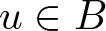
$|a(u)|\leqslant M|u|$, for some positive
$M$. Therefore, we have
(2.4)\begin{align}
|u(t,x)|&\leqslant |u_0(x)|+\Big|\int_0^t\int_A k(x,y)a(u(\tau,y))dy d\tau\Big| \nonumber \\
&\leqslant |u_0(x)|+M\int_0^t\int_A|k(x,y)||u(t,y)|dyd\tau.
\end{align}Define a new function
$v(t,x)=\mu(x)u(t,x)$. Replacing
$u$ in (2.4) by
$v(t,x)/\mu(x)$ and defining
$v_0(x)=v(0,x)$, we get
\begin{equation*}
|v(t,x)|\leqslant |v_0(x)|+\int_0^t M\mu(x)\int_A\frac{|k(x,y)|}{\mu(y)}|v(\tau,y)|dyd\tau.
\end{equation*}Therefore, we have
that is,
\begin{equation*}
|v(t,x)|\leqslant |v_0(x)|+\int_0^t M\mu(x) \int_A\frac{|k(x,y)|}{\mu(y)}\|v(\tau,\cdot)\|_{L^\infty}dyd\tau,
\end{equation*}
\begin{equation*}
\|v(t,\cdot)\|_{L^\infty}\leqslant \|v_0\|_{L^\infty}+c_0\int_0^t \|v(\tau,\cdot)\|_{L^\infty}d\tau.
\end{equation*}The relation above combined with the Gronwall inequality yields
(2.5)\begin{equation}
\|v(t,\cdot)\|_{L^\infty}\leqslant \|v_0\|_{L^\infty}e^{c_0t}.
\end{equation}Since
and
\begin{equation*}\mu(x)|u(t,x)|=|v(t,x)|\leqslant \|v_0\|_{L^\infty}e^{c_0t},\end{equation*}
$v_0(x)=u(0,x)\mu(x)=u_0(x)\mu(x)$, by (1.8) we conclude that
that implies (1.9).
\begin{equation*}
\mu(x)|u(t,x)|\leqslant \|v_0\|_{L^\infty}e^{c_0t}=\gamma e^{c_0t},\end{equation*}























3. Applications of Theorem 1.3
3.1. Classical ODEs in
$\mathbb{R}^n$

Let us first consider the linear Cauchy problem
 \begin{equation}
\left\{
\begin{array}{lcl}
u'(t)&=&Mu(t), \\
\\
u(0)&=&u_0,
\end{array}
\right.
\end{equation}
where  $u(t)=(u^1(t),\ldots,u^n(t))$ is a vector function,
 $M$ is a
 $n\times n$ constant matrix, and
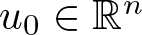 $u_0\in\mathbb{R}^n$ is a fixed point. System (3.1) can be obtained from (1.4) by taking
 $k(x,y)=\delta(x-y)$, where
 $\delta$ means the usual Dirac delta distribution and
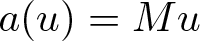 $a(u)=Mu$. In particular, we have
 $|a(u)|\leqslant \|M\||u|$, where
 $\|M\|$ denotes any norm of a matrix we may wish to consider.
Since the problem is purely an ODE in  $\mathbb{R}^n$, it does not have any dependence on any other variable. As a result, if we want to consider a function
 $\mu$ as in Theorem 1.3, it has to be constant. Without loss of generality, we may assume
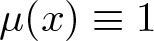 $\mu(x)\equiv 1$. As a result, from (1.6)–(1.8) we get
 \begin{equation}
c_0=\|M\|, \,\,\,c_1=1,\,\,\,\gamma=|u_0|.
\end{equation}
It is well known that the unique solution of (3.1) is given by
 \begin{equation}
u(t)=e^{tM}u_0.
\end{equation}
On the other hand, (1.9) tells us that
 \begin{equation*}\sup_{x\in A}\Big(|u(t,x)|\mu(x)\Big)\leqslant |u_0|e^{t\|M\|},\end{equation*}
which is trivially true for (3.3).
Let us consider a still simple, but more general case than (3.1). Assume that  $a:\mathbb{R}\rightarrow\mathbb{R}$ is a
 $C^1$ locally Lipschitz function with
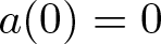 $a(0)=0$ (in particular, it satisfies (1.3)) and consider (1.4) with
 $k(x,y)=\delta(x-y)$, so that it is reduced to
 \begin{equation}
\left\{
\begin{array}{lcl}
u'(t)&=&a(u(t)), \\
\\
u(0)&=&u_0.
\end{array}
\right.
\end{equation}
We again take 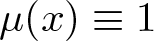 $\mu(x)\equiv1$ and from (1.6) to (1.8) we get
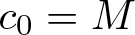 $c_0=M$,
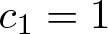 $c_1=1$, and
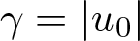 $\gamma=|u_0|$. From Theorem 1.3, the unique solution of (3.4) satisfies
 \begin{equation*}|u(t,x)|\leqslant |u_0|e^{Mt}\end{equation*}
as long as it exists.
Remark 3.1. It is well known that solutions of equations like (3.4) may have a blow-up in finite time, so that it is natural to ask whether it might contradict (1.14). A careful analysis on (2.2) reveals that all of the obtained estimates are valid for  $|u(t,x)-u_0|\leqslant r$ within the interval of existence of the solution. From the proof of Theorem 1.3, this is guaranteed provided that
 \begin{equation*}t\leqslant T{\leqslant}\frac{1}{c_1M}.\end{equation*}
Condition (1.9) is valid for any 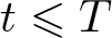 $t\leqslant T$. For
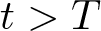 $t \gt T$ our results, a priori, say nothing about what might happen to the solution. For those solutions that experience a blow-up, for some posterior value of
 $t$, it continues existing until it reaches the time
 $t_0$ of the explosion. For some value
 $t_\ast$ beyond
 $T$ but before
 $t_0$ we must have a violation of (1.9), meaning that
 $t_\ast$ is a transition time between a sub-exponential growth of the solution, or we also might call it as sub-blow-up growth, that is the behaviour of the solution before
 $t_\ast$, after which the solution deviates to a new regime, with super-exponential growth, or a blow-up regime, for which although the solution exists, it cannot be dominated by any bound from above. We observe that such a time must occur after the interval of validity of Theorem 1.3.
Let us explore Remark 3.1 in a more concrete way. Consider the Cauchy problem
 \begin{equation}
\left\{
\begin{array}{lcl}
u'(t)&=&u^2, \\
\\
u(0)&=&u_0 \gt 0.
\end{array}
\right.
\end{equation}
Its solution, given by
 \begin{equation}
u(t)=\frac{u_0}{1-tu_0},
\end{equation}
blows-up at 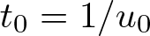 $t_0=1/u_0$. Let us investigate (1.9). Taking
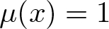 $\mu(x)=1$, we conclude that
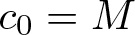 $c_0=M$,
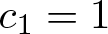 $c_1=1$, and
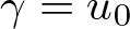 $\gamma=u_0$.
Since 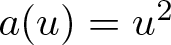 $a(u)=u^2$, then
 \begin{equation*}|a(u)-a(v)|\leqslant |u+v||u-v|\leqslant 2R|u-v|, \,\,\, R=r+\|u_0\|_{L^\infty},\end{equation*}
so that we can take  $M=2R$ and
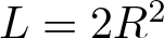 $L=2R^2$. The results given by Theorem 1.3 are then valid for
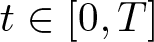 $t\in[0,T]$, where
 \begin{equation*}T{\leqslant}\frac{1}{2R}.\end{equation*}
Let us take a look at (1.9). It says that
 \begin{equation}
\frac{u_0}{1-tu_0}\leqslant u_0e^{2Rt}.
\end{equation}
Let  $z:=2Rt$ and
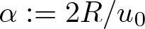 $\alpha:=2R/u_0$. Then the inequality above can be rewritten as
 \begin{equation*}
\alpha\leqslant (\alpha-z)e^{z}.
\end{equation*}
Multiplying the relation above by  $-e^{-\alpha}$, we get
 \begin{equation*}
(z-\alpha)e^{z-\alpha}\leqslant-\alpha e^{-\alpha}.
\end{equation*}
The Lambert  $W$ function is defined as follows:
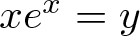 $xe^x=y$ if and only if
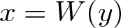 $x=W(y)$. Using such a function, the inequality above tells us that
 \begin{equation*}
z\leqslant \alpha+W(-\alpha e^{-\alpha}),
\end{equation*}
that, returning to the original variables, implies
 \begin{equation*}
t\leqslant \frac{1}{u_0}+\frac{1}{2R}W\Big(-\frac{2R}{u_0}e^{-2R/u_0}\Big)=:t_\ast
\end{equation*}
As a result, since  $e^{-2R/u_0} \lt 1$ and
 $W(z)\approx z+O(z^2)$, we have
 \begin{equation*}
W\Big(-\frac{2R}{u_0}e^{-2R/u_0}\Big)\approx -\frac{2R}{u_0}+\frac{4R^2}{u_0^2},
\end{equation*}
and thus,
 \begin{equation*}t_\ast\approx \frac{2R}{u_0^2} \gt \frac{1}{2R}{\geqslant}T.\end{equation*}
On the other hand, since 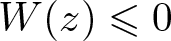 $W(z)\leqslant 0$ for
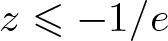 $z\leqslant -1/e$, we conclude that
 \begin{equation*}
T \lt t_\ast \lt \frac{1}{u_0}=t_0,
\end{equation*}
meaning that (1.9) is valid beyond  $T$ until a time
 $t_\ast$ before the blow-up, after which we have another behaviour of the solution.
The growth of the function until  $t_\ast$ is a sub-blow-up growth, whereas after this critical value, the solution experiences a sudden increase, stronger than the exponential one that bounds the function from above before
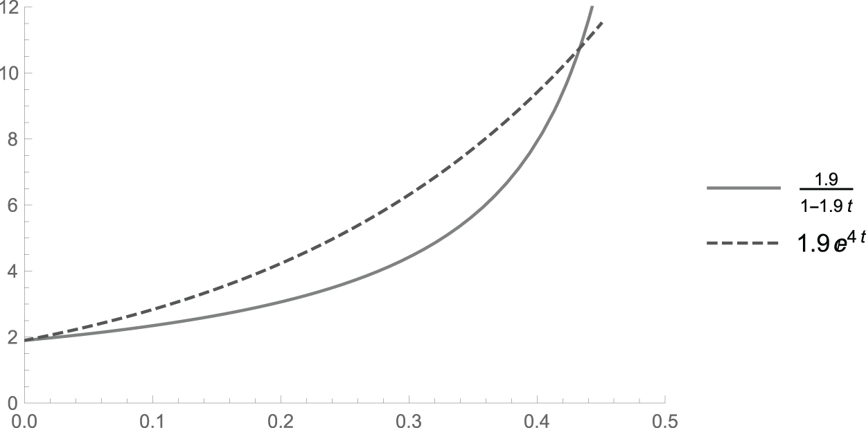
 $t_\ast$, see Figure 2.
Graphs of the solution (3.6) of (3.5) (continuous) and its upper bound (right-hand side of (3.7), in dashed) for 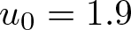 $u_0=1.9$ and
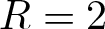 $R=2$. Both curves have an intersection at
 $t\approx 0.4333$. The blow-up occurs at
 $t_0\approx 0.526$. Observe that before this value, we have the inequality (3.7) being satisfied.

3.2. Application to PDEs
Let us consider the Cauchy problem
 \begin{equation}
\left\{
\begin{array}{lcl}
\partial_t u(t,x)&=&a(u(t,x)), \\
\\
u(0,x)&=&u_0(x),
\end{array}
\right.
\end{equation}
where 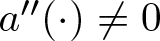 $a''(\cdot)\neq0$ (that ensures non-linear effects),
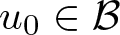 $u_0\in\mathcal{B}$ and
 $\mathcal{B}$ is some Banach space. Once more, system (3.8) can be easily obtained from (1.4) by taking
 $k(x,y)=\delta(x-y)$. Its solution is given by
 \begin{equation*}
A(u):=\int\frac{du}{a(u)}=t+c(x),
\end{equation*}
where the function  $c(x)$ is determined by the initial datum
 $u_0$. In particular,
 $c(x)=A(u(0,x))=A(u_0(x))$. Since
 $A'(u)=1/a(u)\neq0$, we conclude that
 $A$ is either increasing or decreasing and we can locally invert the function
 $A$, so that we have
 \begin{equation*}
u(t,x)=A^{-1}(t+A(u_0(x))).
\end{equation*}
As a result, (1.9) implies that
 \begin{equation*}
|u(t,x)|\leqslant \frac{\gamma e^{c_0t}}{\mu(x)}\leqslant \frac{\gamma e^{c_0t}}{\mu_0},
\end{equation*}
where 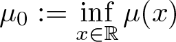 $\mu_0:=\inf\limits_{x\in\mathbb{R}}\mu(x)$.
Consider the equation
 \begin{equation*}
|u(t,x)|=\frac{\gamma e^{c_0t}}{\mu_0}
\end{equation*}
and let 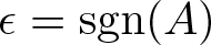 $\epsilon=\text{sgn}{(A)}$. Since
 $A$ is continuous and either increasing or decreasing, it is locally one sign and the above implies
 \begin{equation*}
A^{-1}(t+A(u_0(x)))=\epsilon\frac{\gamma}{\mu_0}e^{c_0t},
\end{equation*}
that is,
 \begin{equation}
t+A(u_0(x))=A\Big(\epsilon\frac{\gamma}{\mu_0}e^{c_0t}\Big),
\end{equation}
that can be solved for  $t$ in terms of
 $x$, that is, we have
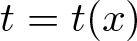 $t=t(x)$. The value
 \begin{equation*}t_\ast=\inf_{x\in\mathbb{R}}t(x),\end{equation*}
where  $t(x)$ solves (3.9), gives the bound for
 $t$ for which (1.9) is no longer valid beyond this value. More concretely, let us specify
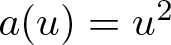 $a(u)=u^2$ and take now
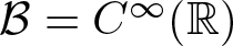 $\mathcal{B}=C^\infty(\mathbb{R})$, so that we can compare this case with that in the previous section.
A straightforward calculation shows that the solution of (3.8) with 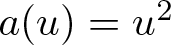 $a(u)=u^2$ is
 \begin{equation}
u(t,x)=\frac{u_0(x)}{1-tu_0(x)}.
\end{equation}
If 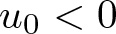 $u_0 \lt 0$, then (3.10) exists and is bounded for all
 $t \gt 0$. Otherwise, it experiences a blow-up at
 \begin{equation}
t_0:=\inf_{x\in\mathbb{R}}\Big\{\frac{1}{u_0(x)},\,\,u_0(x) \gt 0\Big\}
\end{equation}
For a positive initial datum  $u_0$, the solution exists for
 $t$ given by (3.7), replacing
 $1/u_0$ by
 $t_0$ in (3.11).
Let us now assume that (1.8) holds for some  $\mu$. We again have the validity of (1.9) and then, from (1.7), we can take
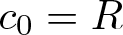 $c_0=R$.
From (1.9), we infer that
 \begin{equation}\frac{u_0(x)}{1-tu_0(x)}=u(t,x)\leqslant\frac{\gamma e^{2Rt}}{\mu(x)}.\end{equation}
Suppose we have
 \begin{equation*}
\frac{u_0(x)}{1-tu_0(x)}=\frac{\gamma e^{2Rt}}{\mu(x)}.
\end{equation*}
Let  $z:=2Rt$. Then, after rearranging terms once more, we get
 \begin{equation*}
\Big(z-\frac{2R}{u_0(x)}\Big)e^z=-\frac{2R\mu(x)}{\gamma}.
\end{equation*}
Defining  $y:=z-2R/u_0(x)$, the last equation implies
 \begin{equation*}
ye^y=-\frac{2R}{\gamma}\mu(x)e^{-\frac{2R}{u_0(x)}},
\end{equation*}
meaning that
 \begin{equation*}
y=W\Big(-\frac{2R}{\gamma}\mu(x)e^{-\frac{2R}{u_0(x)}}\Big),
\end{equation*}
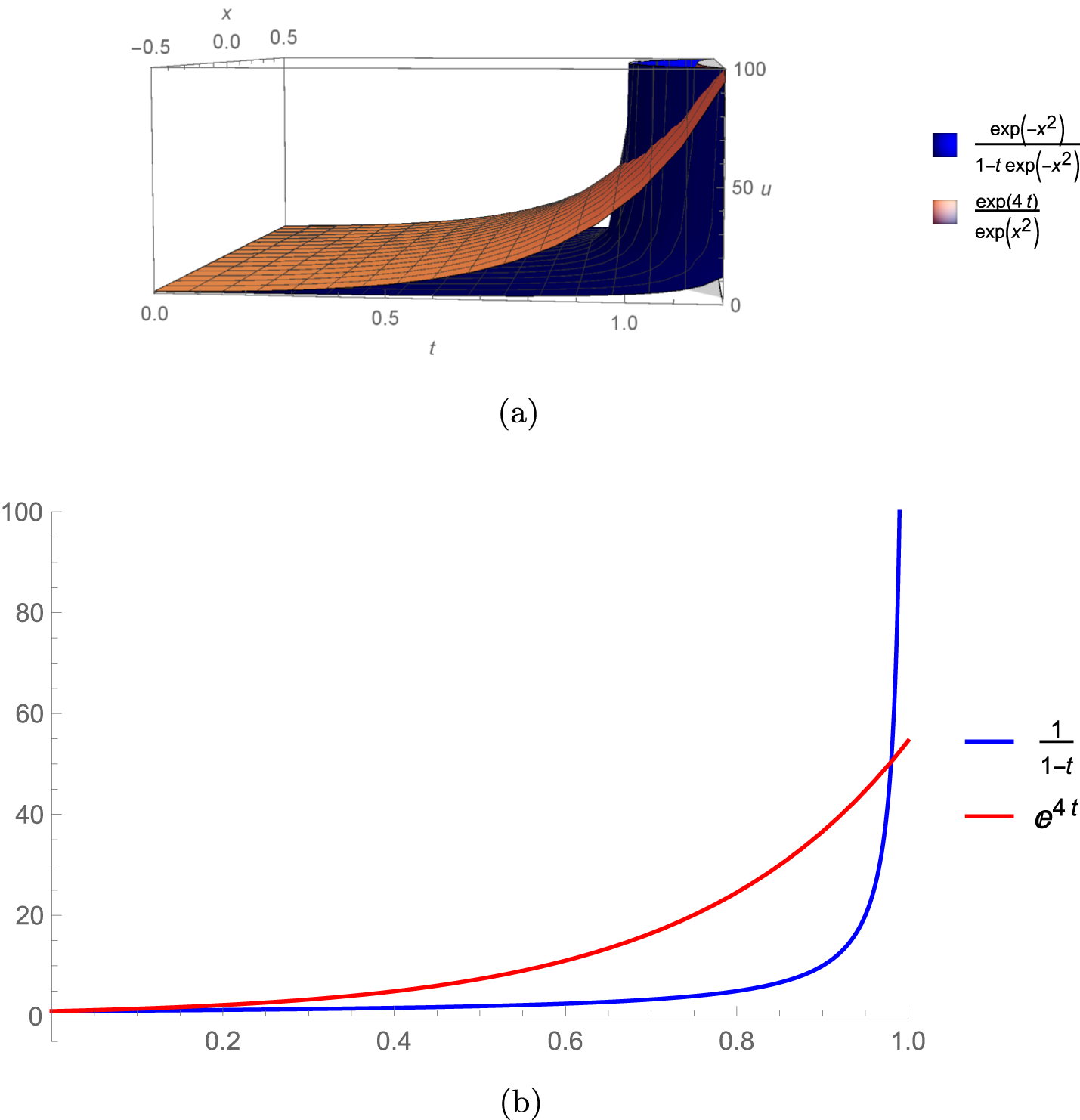
that, solved for  $t$, gives (see Figure 3)
 \begin{equation}
t(x)=\frac{1}{u_0(x)}+\frac{1}{2R}W\Big(-\frac{2R}{\gamma}\mu(x)e^{-\frac{2R}{u_0(x)}}\Big).
\end{equation}
Behaviour of the solution (3.10) and the upper bound (3.12). The solution becomes greater than in the region  $(t,x)$, for
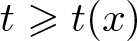 $t\geqslant t(x)$, where
 $t(x)$ is given by (3.13). For
 $x=0$, the point determining the change of behaviour is
 $t(0)\approx 0.9802$, while the blow-up occurs at
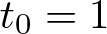 $t_0=1$. (a) Solution (3.10) with
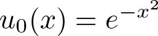 $u_0(x)=e^{-x^2}$ (in blue) and the right-hand side of (3.12) with
 $\gamma=1$,
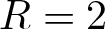 $R=2$ and
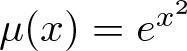 $\mu(x)=e^{x^2}$ (in light red). (b) Profile of the function in Figure 3(a) for
 $x=0$.

4. Proof of Theorem 1.7 and applications
We first note that (1.12) falls into the class (1.4). Moreover, under the conditions on  $a$,
 $a(u)\in H^s(\mathbb{R})$ as long as
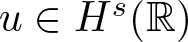 $u\in H^s(\mathbb{R})$,
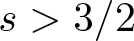 $s \gt 3/2$, e.g., see [Reference Taylor13, Exercise 8 on p. 320] or [Reference Constantin and Molinet7, Lemma 1]. As a result, the function
 $a$ satisfies (1.3) and we have granted the conditions for ensuring the existence of a local solution
 $u\in C^0([0,T];H^s(\mathbb{R}))$, for some
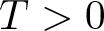 $T \gt 0$.
Let  $\gamma$ be given by the left-hand side of (1.13). What remains to be done is finding the constants
 $c_0$ and
 $c_1$.
4.1. Proof of the theorem
What remains to be proved is precisely the persistence property (1.14) or (1.15) under the assumption (1.13).
We divide the remaining proof of Theorem 1.7 in three major parts:
• We first prove it for the non-periodic case when
$n=1$.• Next we prove it for the periodic case when
$n=1$.• Then we treat
$n \gt 1$ for both periodic and non-periodic cases.


4.1.1. Non-periodic case for
$n=1$

In this case, we have
 \begin{equation}
\partial_xg(x)=-\frac{\text{sgn}{(x)}e^{-|x|}}{2}.
\end{equation}
Since 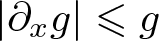 $|\partial_xg|\leqslant g$, let us define
 \begin{equation}
F(x)=\mu(x)\int_{\mathbb{R}}\frac{g(x-y)}{\mu(y)}dy,
\end{equation}
where  $g$ is given by (1.10) and
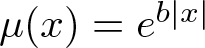 $\mu(x)=e^{b|x|}$. Since
 $g$ and
 $\mu$ are even functions, so is
 $F$. Without any loss of generality, we can estimate
 $F(x)$ for non-negative values of
 $x$, see also [Reference Bona, Chen, Hong, Panthee and Scialom2, p. 5]. Indeed,
 \begin{align}
2F(x)&= \int_{-\infty}^0 e^{-bx-x+y+by}dy \nonumber\\
& \quad+\int_0^x e^{bx-x+y-by}dy+\int_x^\infty e^{bx+x-y-by}dy \nonumber\\
&=\frac{2(1-be^{-(1-b)x})}{1-b^2}\leqslant \frac{2}{1-b^2}.
\end{align}
Therefore, we can take
 \begin{equation}
c_0= \frac{M}{1-b^2},\quad c_1=1.
\end{equation}
4.1.2. Periodic case for
$n=1$

We proceed similarly as in the non-periodic case, but now we replace  $F$ in (4.2) by (see (1.10))
 \begin{align}
F(x)&=\frac{e^{bx+1/2}}{2\sinh{\frac{1}{2}}}\int_0^1 e^{x-(1+b)y}dy\leqslant \frac{1}{b+1}\frac{e^{b+5/2}-e^{2b+7/2}}{(b+1)(e-1)} \nonumber\\
&=\frac{e^{b+2}}{(b+1)(e-1)}(e-e^{b+2})\leqslant \frac{e^{b+2}}{b+1},
\end{align}
wherefrom we can take
 \begin{equation}
c_0=Me^{b+2}.
\end{equation}
Moreover, we have
 \begin{equation*}
c_1=\int_0^1\frac{\cosh{(x-\frac{1}{2})}}{2\sinh{\frac{1}{2}}}dx=1.
\end{equation*}
Again, the result follows from (1.13) and (1.12). We can extend (1.13) to any 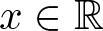 $x\in\mathbb{R}$, replacing
 $x$ by
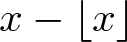 $x-\lfloor x \rfloor $, that gives (1.14). This extension, however, possesses issues when evaluated on integers, since
 $\tilde{\mu}(x):=\mu(x-\lfloor x \rfloor)$ and
 $g$ are not differentiable at
 $x=n\in\mathbb{Z}$.
4.2. Application to the classical BBM equation
It is well known that (1.12) is well-posed in Sobolev spaces and, in particular, for 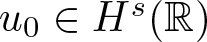 $u_0\in H^s(\mathbb{R})$,
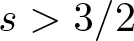 $s \gt 3/2$, we have
 $\|u(t,\cdot)\|_{H^1(\mathbb{R})}\leqslant \|u_0\|_{H^1(\mathbb{R})}$. As a result, the Sobolev Embedding Theorem guarantees that
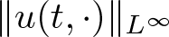 $\|u(t,\cdot)\|_{L^\infty}$ is bounded within the interval of existence of the solution, e.g, see [Reference da Silva and Freire8] and references therein.
Let us take  $a(u)=u+u^2/2$ in order to recover the original form of the BBM equation [Reference Benjamin, Bona and Mahony1]. From the above observations, we have
 $M=1+\|u_0\|_{H^1(\mathbb{R})}$ in (1.3) and (1.14) reads
 \begin{equation}
|u(t,x)|\leqslant \gamma e^{\frac{1+\|u_0\|_{H^1(\mathbb{R})}}{1-b^2}t-b|x|}.
\end{equation}
In [Reference Bona, Chen, Hong, Panthee and Scialom2], a similar result was established, but our constants are slightly different. More precisely, the difference resides in the fact that our estimated speed is slightly faster than that found by Bona et al. This difference comes from the fact that in [Reference Bona, Chen, Hong, Panthee and Scialom2] they used a specific function and worked on it, while in the present paper we are addressing the equation in a more general form. We can, however, get back the results from [Reference Bona, Chen, Hong, Panthee and Scialom2] using the following remark.
Remark 4.1. If  $a(u)=u\alpha(u)$, for some continuously differentiable function
 $\alpha:\mathbb{R}\rightarrow\mathbb{R}$ (not necessarily satisfying the condition
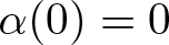 $\alpha(0)=0$), then (2.4) can be replaced by
 \begin{align}
|u(t,x)|&\leqslant |u_0(x)|+\Big|\int_0^t\int_A k(x,y)a(u(\tau,y))dy d\tau\Big| \nonumber \\
&\leqslant |u_0(x)|+\sup_{|z|\leqslant R}|\alpha(z)|\int_0^t\int_A|k(x,y)||u(t,y)|dyd\tau,
\end{align}
where  $R=r+\|u_0\|_{L^\infty(\mathbb{R})}$.
Therefore, from (4.8), we get back (2.5), where  $c_0$ is given by (1.7) with
 \begin{equation*}M=\sup\limits_{|z|\leqslant R}|\alpha(z)|.\end{equation*}
4.3. BBM system
Consider the following system, deduced in [Reference Bona and Chen3]:
 \begin{equation}
\left\{\begin{array}{l}
u_t+v_x+(uv)_x-\frac{1}{6}u_{txx}=0,\\
\\
v_t+u_x+vv_x-\frac{1}{6}v_{txx}=0.
\end{array}
\right.
\end{equation}
Let  $(u_0,v_0)\in H^s(A)\times H^s(A)$,
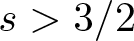 $s \gt 3/2$. If we change
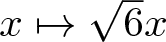 $x\mapsto \sqrt{6}x$ and invert the operator
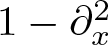 $1-\partial_x^2$, then (4.9) endowed with the conditions
 $(u,v)|_{t=0}=(u_0,v_0)$ can be rewritten as
 \begin{equation}
\left\{\begin{array}{l}
u_t+\frac{1}{\sqrt{6}}\partial_x g\ast (v+uv)=0,\\
\\
v_t+\frac{1}{\sqrt{6}}\partial_x g\ast (u+v^2)=0.
\end{array}
\right.
\end{equation}
By the Sobolev Embedding Theorem and the algebra property,  $u,v,uv,v^2\in H^s(A)$, meaning that the terms involving convolutions are continuous. By Theorem 1.3, we have a local solution
 $(u,v)$. Therefore, provided that (1.13) holds, then we have (1.14), where
 $\gamma=\sup\limits_{x\in A}(e^{b|x|}(|u_0(x)|{+|v_0(x)|})$ and
 $c_0$ is twice the values obtained in (4.4) or (4.6), depending on whether
 $A=\mathbb{R}$ or
 $A=\mathbb{S}$, respectively.
5. Proof of Theorem 1.8
Let us now consider the following equation
 \begin{equation}
u_{tt}=\partial_x^2f(u)+u_{ttxx},
\end{equation}
with 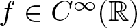 $f\in C^\infty(\mathbb{R})$ and
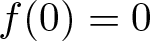 $f(0)=0$.
Well-posedness results for the improved Boussinesq ( $f(u)=u-u^2$ above) were established in [Reference Turitsyn14], as well as its blow up. More recently, Constantin and Molinet in [Reference Constantin and Molinet7] proved the existence and uniqueness of solutions for (5.1) under the same restrictions on
 $f$ that we are using in this paper.
In [Reference Constantin and Molinet7, Theorem 1], it was established local existence of solutions for (5.1) subject to
 \begin{equation}
u(0,x)=u_0(x),\,\,\,\,u_t(0,x)=v_0(x).
\end{equation}
Provided that they belong to  $H^s(\mathbb{R})\cap L^\infty(\mathbb{R})$,
 $s\geqslant 0$, then (5.1) subject to (5.2) has a unique solution
 $u\in C^2([0,T);H^s(\mathbb{R})\cap L^\infty(\mathbb{R}))$.
Let us then assume  $u\in C^2([0,T);H^s(\mathbb{R})\cap L^\infty(\mathbb{R}))$, for some
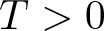 $T \gt 0$, and
 $s\geqslant 0$, as a solution of (5.1). Defining
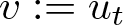 $v:=u_t$, using that
 $\partial_x^{2}\Lambda^{-2}=\Lambda^{-2}-1$,
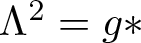 $\Lambda^{2}=g\ast$, we can rewrite (5.1)–(2.5) as (for further details, see [Reference Constantin and Molinet7, p. 1066])
 \begin{equation}
\left\{
\begin{array}{lcl}
u_t&=&v,\\
\\
v_t&=&g\ast f(u)-f(u),\\
\\
u(0,x)&=&u_0(x),\\
\\
v(0,x)&=&v_0(x),
\end{array}\right.
\end{equation}
that falls into (1.4) with  $k=(\delta(x-y),g(x-y)-\delta(x-y))$, where
 $g$ is given by (1.10), and
 $a(u,v)=(v,f(u))$.
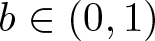
Suppose that 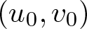 $(u_0,v_0)$ satisfies (1.17), for some
 $b\in(0,1)$, and
 \begin{equation*}\gamma=\sup_{x\in\mathbb{R}}\Big[e^{b|x|}\Big(|u_0(x)|+|u_1(x)|\Big)\Big].\end{equation*}
Let  $r \gt 0$ be the radius of a closed ball
 $B$ with centre
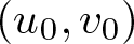 $(u_0,{v_0)}$ for which we have the local solution of (5.3) lying in and
 $R=r+\|u_0\|_{L^\infty}+\|v_0\|_{L^\infty}$. Then, if
 $(u,v),\,(\overline{u},\overline{v})\in B$, we have
 \begin{align*}
|a(u,v)-a(\overline{u},\overline{v})|&=|f(u)-f(\overline{u})|+|v-\overline{v}|\\
&\leqslant \Big(1+\sup_{|z|\leqslant R}|f'(z)|\Big)\Big(|u-\overline{u}|+|v-\overline{v}|\Big)=: M|(u,v)-(\overline{u},\overline{v})|.
\end{align*}
Once more, we use (4.3) to find
 \begin{equation*}c_0=\frac{3-2b^2}{1-b^2}M,\end{equation*}
that gives (1.18)
Acknowledgements
This work was supported by FAPESP (grant number 2024/01437-8) and CNPQ (grant number 310074/2021-5).