Introduction
Multilayer graphene structures have promising applications in antennas, sensors, and absorbers [Reference Geim and Novoselov1–Reference Francescato, Giannini, Yang, Huang and Maier5]. Chemical potential of graphene can be tuned through electrostatic doping. Thus, graphene can become a basic element in the creation of tunable devices.
Photonic crystal based on multilayer graphene structure at terahertz frequencies have been proposed in [Reference Berman, Boyko, Kezerashvili, Kolesnikov and Lozovik6, Reference Berman and Kezerashvili7]. Few-layer graphene flakes with <10 layers each show a distinctive band structure in 0.9–1.3 THz [Reference Tan, Han, Zhao, Wu, Chang, Wang, Wang, Bonini, Marzari, Pugno, Savini, Lombardo and Ferrari8].
In a large number of papers, graphene strips are analyzed with the use of the finite-difference method [Reference Nayyeri, Soleimani and Ramahi9, Reference Chen, Li and Liu10]. However, such a method has significant restrictions on the size of the structure under study. The approximate radiation conditions bound the accessible accuracy.
Graphene layer can be considered as a dielectric with certain permittivity and thickness. Still the accuracy of such a model degrades as Δ/λ increases, where Δ is the thickness of the graphene layer and λ is the wavelength [Reference Shao, Yang and Huang11]. In [Reference Zhao, Tao, Ding and Chen12], a dispersive time-domain method is used to study properties of graphene arrays. Based on the time-domain volume integral equation method, the volume integrals are converted into surface integrals. Drude formula is used to model the conductivity of graphene and as a consequence to model its permittivity. The discrepancy between graphene dielectric function extracted from Kubo formulism and Drude model is demonstrated, for example, in [Reference Hosseininejad and Komjani13].
Method of moments [Reference Burghignoli, Araneo, Lovat and Hanson14], finite element method [Reference Huang, Wu, Tang and Mao15], discontinuous Galerkin time-domain method [Reference Li, Jiang and Bagct16] also can be applied to study the graphene gratings. In [Reference Fuscaldo, Burghignoli, Baccarelli and Galli17], a customized efficient circuit model is employed to study a single unpatterned graphene sheet placed inside a grounded dielectric multilayer. In [Reference Zinenko, Matsushima and Nosich18], infinite periodic graphene grating placed into dielectric slab is studied with the use of the regularizing method of moments. Three types of resonances are identified: the resonance on the localized surface-plasmon modes, the grating modes, and the slab modes.
In [Reference Kaliberda, Lytvynenko and Pogarsky19], finite system of layers is analyzed with the use of the singular integral equations method. With the number of scatterers increases, the dimension of the matrix is also increased. It leads to significant increase of calculations time. Thus it makes sense to divide complex structure into several similar substructures and to analyze every substructure separately. Contrary to the methods when the structure is analyzed as a whole, such approach allows to reduce the dimension of the resulting system of lineal algebraic equations and decrease the computation time. The method of S-matrix allows to obtain the scattering matrix of a system which consists of a finite number of layers if the properties of a single layer are known. In [Reference Hwang20], finite number of bi-periodic graphene layers is cascaded with the use of the S-matrix approach. In [Reference D'Aloia, D'Amore and Sarto21], absorbing structure which consists of a two-period dielectric Salisbury screen backed with a perfect electric conducting (PEC) metal plate is considered with the similar approach. The first lossy sheet is an undoped graphene monolayer, the second lossy sheet is made by a graphene/dielectric laminate. S-matrix approach can be efficiently applied to the scattering by infinite gratings. Obtained equations are the matrix ones. Far less frequently such approach is used to the structures with finite dimensions. Here, the obtained equations are the integral ones.
In [Reference Kaliberda, Litvinenko and Pogarskii22, Reference Lytvynenko, Kaliberda and Pogarsky23], multilayer structures of PEC planar scatterers are considered. The properties of the whole structure are obtained from equations, which are written in the operator form. These equations use the scattering operators of a single layer. In this paper, we are going to use the same approach to analyze multilayer system of identical graphene planar strip gratings. To describe the graphene, we use the model of zero-thickness impedance sheet, characterized with surface conductivity via the Kubo formalism.
Solution of the problem
Basic notations
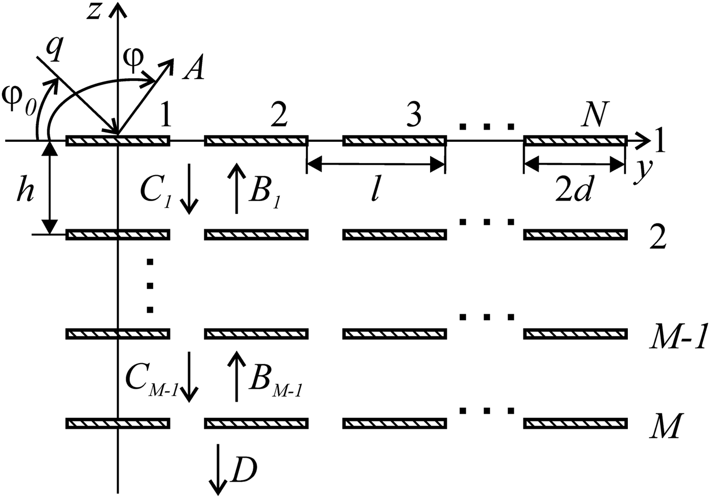
Consider graphene grating represented in Fig. 1. The geometry of the structure is characterized with the following parameters: period l, strip width 2d, distance between layers h, number of strips in every layer N, and number of layers M. The strips are infinite along the x-axis and are placed in the free space. Graphene strip can be characterized with chemical potential μ c, relaxation time τ, and temperature T. The surface conductivity of graphene σ is obtained using the Kubo formalism [Reference Hanson24, Reference Hanson25]. Note that for the parameters of graphene considered in this paper for the considered frequency band, the intraband contributions dominate and interband transitions is small [Reference Zinenko, Matsushima and Nosich18].
Structure geometry.

We describe the incident H-polarized field as a Fourier integral (a spectrum of plane waves) with spectral function q(ξ),
 $$H_x^i (y,z) = \int\limits_{ - \infty} ^\infty {q(\xi )\exp (ik(\xi y - \gamma (\xi )z))d\xi}, $$
where  $\gamma (\xi ) = \sqrt {1 - \xi ^2} $,
 ${{\rm Re}} \gamma \ge 0$,
 ${{\rm Im}} \gamma \ge 0$, and k = 2π/λ is the wavenumber, q(ξ) is known amplitude. If only a single plane wave is incident under the angle φ 0 then q(ξ) = δ(ξ − cosφ 0), where δ(ξ) is the Dirac delta function. The total field we represent as a superposition of the incident and scattered fields. It should satisfy the Helmholtz equation, the following boundary conditions:
 $$E_y^ + = E_y^ -, $$
 $$\displaystyle{1 \over 2}\lpar {E_y^ + + E_y^ -} \rpar = \displaystyle{1 \over \sigma} \lpar {H_x^ + - H_x^ -} \rpar .$$
Also the radiation and the edge conditions should be satisfied.
We present the scattered field as Fourier integral with spectral functions A(ξ), C m(ξ), B m(ξ), and D(ξ), m = 1, 2, …, M − 1 (directions of wave propagation are shown in Fig. 1).
Single layer of graphene strips
In this section, we describe briefly the method of singular integral equations for a single layer placed in the z = 0 plane [Reference Kaliberda, Lytvynenko and Pogarsky26]. Denote the set of strips as  $L = \bigcup\nolimits_{n = 1}^N {( - d + l \cdot n;\,d + l \cdot n)} $. Incident field is described by (1). Scattered field we seek as
 $$H_x^s (y,z) = {{\rm sgn}} (z)\mathop {\int}\limits_{ - \infty} ^\infty {C(\xi )\exp (ik\xi y + ik\gamma (\xi ) \vert z \vert )d\xi}, $$
where C(ξ) is unknown spectral function. It satisfies the Helmholtz equation, the radiation condition, and (2). From (2) and (3) we may obtain following dual integral equations:
 $$\int\limits_{ - \infty} ^\infty {C(\xi )\exp (ik\xi y)d\xi} = 0,\quad y \notin L,$$
 $$\eqalign{&\displaystyle{{2ik} \over {\sigma Z}}\mathop{\int}\limits_{ - \infty} ^\infty {C(\xi )\exp (ik\xi y)d\xi} + ik\mathop{\int}\limits_{ - \infty} ^\infty {\gamma (\xi )C(\xi )\exp (ik\xi y)d\xi} \cr&\quad = - \displaystyle{\partial \over {\partial z}}H_x^i (y,0),\quad y \in L.$$
Introduce function  $F(y) = ik\int_{ - \infty} ^\infty {\xi C(\xi )\exp (ik\xi y)d\xi} = 0$. From (4) it follows that F(y) is up to a constant factor the derivation of the current density on the strips. Then
 $$C(\xi ) = \displaystyle{1 \over {2\pi \,i\xi}} \int\limits_L {F(y)(\exp (iky\xi ) - 1)dy}. $$
In (6), let us represent function  $\gamma (\xi ) = \sqrt {1 - \xi ^2} \sim i\vert \xi \vert + O(1/\xi )$, ξ → ∞, as a sum of vanishing and non-vanishing terms, γ(ξ) = (γ(ξ) − i|ξ|) + i|ξ| and use the Hilbert transform to the non-vanishing term. The Hilbert transform is
 $$PG(y) = \displaystyle{1 \over \pi} PV\int\limits_{ - \infty} ^\infty {\displaystyle{{G(\xi )} \over {\xi - y}}d\xi}, $$
 $$P\exp (ik\zeta y) = i{{\rm sgn}} (k\zeta )\exp (ik\zeta y),$$
where G(ξ) is an arbitrary function. As a result after transformations singular integral equation can be obtained
 $$\eqalign{&\displaystyle{1 \over \pi} PV\int\limits_L {\displaystyle{{F(\xi )} \over {\xi - y}}} d\xi + \displaystyle{1 \over \pi} \int\limits_L {K(y,\xi )F(\xi )d\xi} = - \displaystyle{\partial \over {\partial z}}H_x^i (y,0),\cr& y \in L.}$$
The additional conditions follow from (5)
 $$\displaystyle{1 \over \pi} \int\limits_{ - d + l \cdot n}^{d + l \cdot n} {F(\xi )d\xi} = 0,\quad n = 1,2, \ldots, N,$$
where PV means Cauchy principal value integral, the kernel function is
 $$K(y,\xi ) = k\int\limits_0^\infty {\displaystyle{{\sin (k\zeta (y - \xi ))} \over \zeta} (\zeta + i\gamma (\zeta ))d\zeta} + q(y,\xi ),$$
 $$q(y,\xi ) = \left\{ {\matrix{ {\displaystyle{{2ik\pi} \over {\sigma Z}},} & {\xi \le y,} \cr {0,} & {\xi \gt y.} \cr}} \right.$$
The numerical solution of (8) and (9) with (10) can be obtained using the Nystrom-type method of discrete singularities [Reference Gandel and Kononenko27].
Let us introduce the transmission t and reflection r integral operators of a single layer of graphene strips,
 $$(tq)(\xi ) = \int\limits_{ - \infty} ^{ + \infty} {t(\xi, \zeta )q(\zeta )d\zeta}, $$
 $$(rq)(\xi ) = \int\limits_{ - \infty} ^{ + \infty} {r(\xi, \zeta )q(\zeta )d\zeta}, $$
where t(ξ, ζ) and r(ξ, ζ) are the kernel functions. These operators connect the Fourier amplitude of incident field (as functions of ζ) with the Fourier amplitude of the scattered field (as functions of ξ). In case if solution of (8) and (9) is known, then C(ξ) can be obtained from (7). Then, for the incident field (1) it follows:
 $$(rq)(\xi ) = C(\xi ).$$
In the H-polarization case, one can write the following relation which connects the kernel functions of the transmission and reflection operators
 $$t(\xi, \zeta ) = \delta (\xi - \zeta ) - r(\xi, \zeta ).$$
From the edge condition it follows that  $H_x^s (y,0) \sim \sqrt {(y - ( - d + l \cdot n))(d + l \cdot n - y)} $, when y approaches the edges of the nth strip. Then, the function C(ξ) as a Fourier transform of
 $H_x^s (y,0)$ satisfies the relation
 $\vert {C(\xi )} \vert \sim \vert \xi \vert ^{ - 3/2}$, when ξ → ∞. From (12) and reciprocity principle it follows that
 $$r(\xi, \zeta ) \sim \vert \xi \vert ^{ - 3/2} \quad {\rm and} \quad r(\xi, \zeta ) \sim \vert \zeta \vert ^{ - 3/2}.$$
Let us consider a finite system of layers.
Multilayer grating
We represent integral equations relatively unknown spectral functions (Fourier amplitudes) of the scattered field in the operator form. The spectral functions of the scattered field are connected as follows:
 $$A = rq - reB_1 + eB_1,$$
 $$B_1 = q - rq + reC_1,$$
 $$C_1 = reB_1,$$
 $$B_m = eB_{m + 1} - reB_{m + 1} + reC_m,$$
 $$C_m = reB_m - reC_{m - 1} + eC_{m - 1},\quad m = 2,3, \ldots, M - 2,$$
 $$B_{M - 1} = reC_{M - 1},$$
 $$C_{M - 1} = reB_{M - 1} - reC_{M - 2} + eC_{M - 2},$$
 $$D = eC_{M - 1} - reC_{M - 1},$$
where the operator e, eg = exp (ikγ(ξ)h)g(ξ), defines the transformation of plane waves on their way through the gap h between the layers. Equation (15) means that reflected field can be represented as a superposition of two fields with amplitude rq and − reB 1 + eB 1. The first one is the field with amplitude q reflected from a single isolated layer of graphene strips. As a result the field with amplitude rq is obtained. Another one is the field with amplitude eB 1 transmitted through the first isolated layer. Taking into account relation between transmission and reflection operators (13) the field with amplitude − reB 1 + eB 1 is obtained. Using the same considerations, one can write (16)–(22).
From (14), it follows that  $\left \Vert r \right \Vert _2 \lt \infty $, where
 $\left \Vert \cdot \right \Vert_2$ is the norm in L 2. Thus r is the Fredholm operator and equations (15)–(22) are the set of the Fredholm integral equations of the second kind. Notice however, that the convergence of (15)–(22) depends on the convergence of numerical method for the operator r. Reflection operator r is obtained from the singular integral equation with additional conditions but not the Fredholm one. Equations (9) and (10) are solved using the Nystrom-type interpolation algorithm. It guarantees the convergence thanks to the theorems on approximation of singular integrals with quadratures [Reference Gandel and Kononenko27].
Using (11), operator equations (15)–(22) can be rewritten in the form of integral equations. The interval of integration is infinite. Taking into account exponentially decaying term exp (ikγ(ζ)h), if |ζ| >1, we can truncate the infinite interval of integration changing it to ( − a;a). After that the compound Gaussian quadrature is applied.
Numerical results
As a rule, to characterize the scattering and absorption by a finite graphene grating, the total scattering cross-section (TSCS) and the absorption cross-section (ASC) are introduced. Suppose that plane wave with unit amplitude is incident on the grating at the angle of incidence φ 0 = 900. The parameters of graphene are μ c = 0.3 eV, τ = 1 ps, T = 300 K. Let us study the convergence. As a reference solution we use the solution from [Reference Kaliberda, Lytvynenko and Pogarsky19].
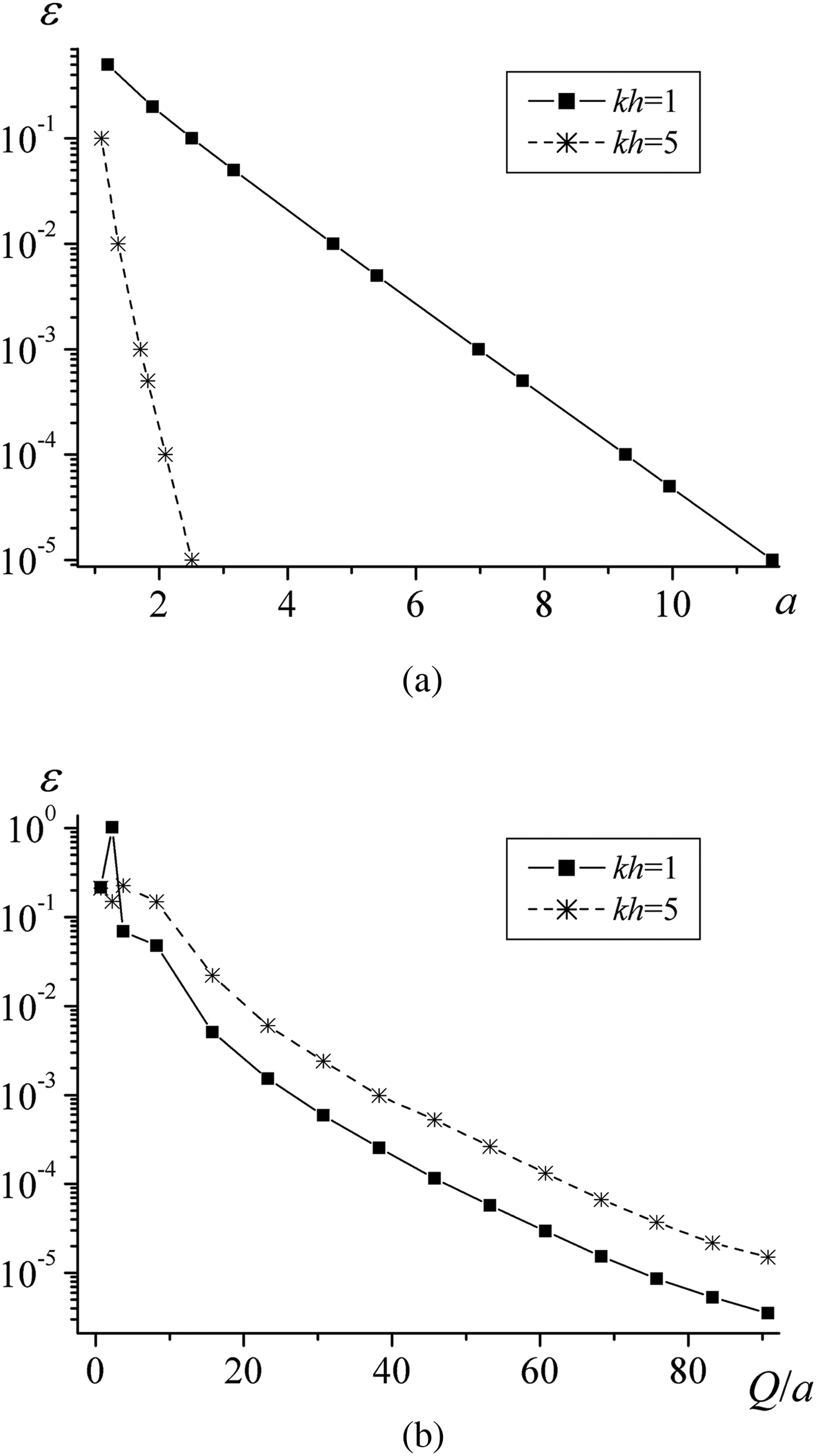
Introduce relative error of TSCS as follows: ε = |TSCS − TSCS SIE|/|TSCS SIE|, where TSCS is obtained from (15)–(22), and TSCS SIE is obtained from [Reference Kaliberda, Lytvynenko and Pogarsky19]. Notation SIE means singular integral equations. The error of the solution mainly depends on the length of the truncated finite interval of integration 2a and on the total number of nodes in the quadrature rule Q. Figure 2 shows dependences of relative error ε versus a and Q. It is obvious that with the parameter a increase we should take larger Q. Thus we consider the number of nodes per length, Q/a, in Fig. 2(b). Since the term exp (ikγ(ζ)h) mainly affects the integrands behavior at infinity, ζ → ∞, we can decrease a exponentially when kh is increased, but a >1. Since the method has guaranteed convergence, the accuracy can archive the level of machine precision. Note that the method used in our paper has been validated in [Reference Kaliberda, Lytvynenko and Pogarsky26] for a planar graphene strip grating by comparison with numerical results obtained using a different algorithm in [Reference Shapoval, Gomez-Diaz, Perruisseau-Carrier, Mosig and Nosich28].
Relative error versus (a) a and (b) Q/a.

The structure under study can support various resonances. In particular, we study the surface plasmon resonances which depend on the parameters of individual strip such as conductivity and width, the resonances near the Rayleigh anomaly caused by the planar grating periodicity, and resonances of a layered grating. First, let us study dependences of the scattering and absorption characteristics as functions of frequency. Then, we consider the influence of the resonances on the far field. Finally, we present dependences of TSCS and ACS as functions of the distance between layers near several resonances.
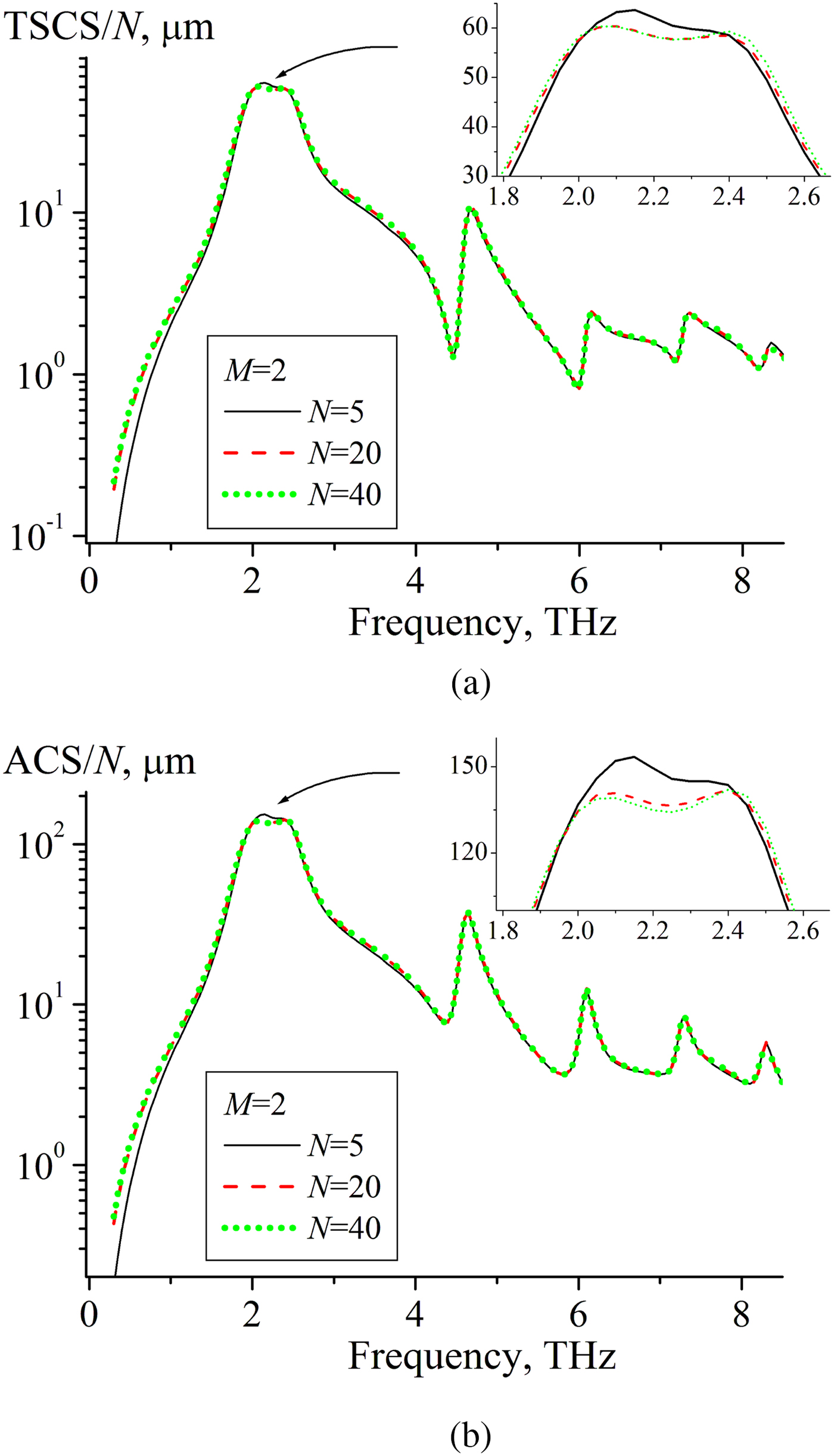
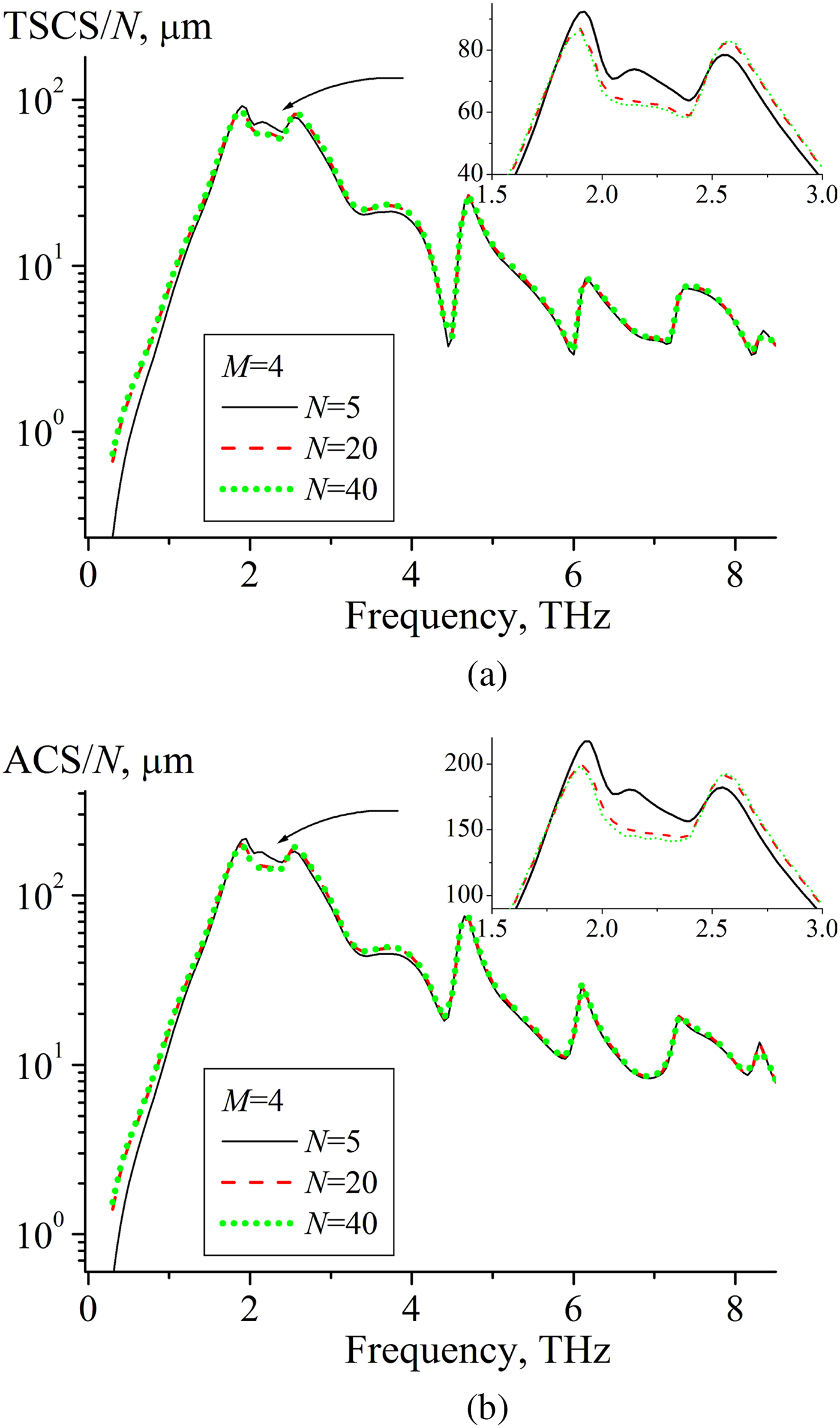
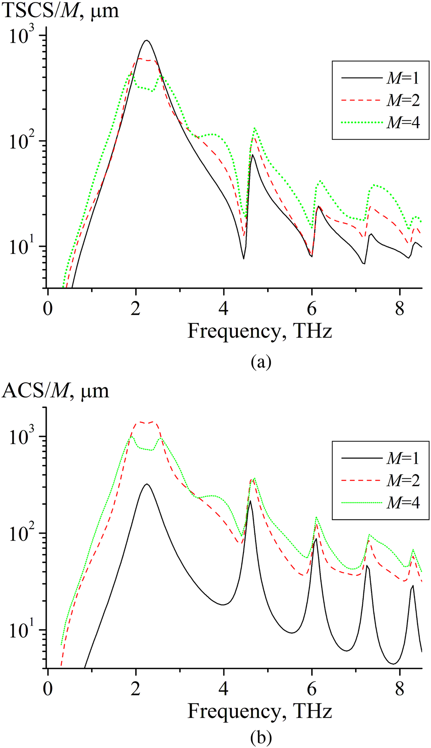
Figures 3–5 show dependences of the normalized TSCS and ACS versus frequency for different number of layers M and different number of strips N in every layer. Frames show zoomed area near the first plasmon resonance. In the case of a single graphene strip or planar grating of graphene strips, the rapid growth of the TSCS and ASC is observed near the plasmon resonances [Reference Kaliberda, Lytvynenko and Pogarsky26, Reference Shapoval, Gomez-Diaz, Perruisseau-Carrier, Mosig and Nosich28]. In the case of a layered graphene structure, another situation can be observed. As one can see from Fig. 5, with the increase of the number of layers, the value of the scattering coefficient per layer (TSCS/M) decreases near frequency of the first plasmon resonance, f = 2.25 THz. Here TSCS is partially suppressed by the interaction between the layers.
Dependences of (a) TSCS and (b) ACS on the frequency for M = 2 layers, N = 5 (solid curves), N = 20 (dashed curves), and N = 40 (dotted curves), μ c = 0.3 eV, τ = 1 ps, T = 300 K, d = 10 μm, h = l = 40 μm. Note the resonances on the surface-plasmon modes of each graphene strip.

Same study as in Fig. 3 but for M = 4 layers.


As one can know, in layered periodic structures the resonances may arise with period kh ≈ π. The first resonance of the graphene layered structure under study is observed near f ≈ 3.8 THz, the second one is near f ≈ 7.6 THz. Notice that the frequency of the second resonance is close to the Rayleigh anomaly. Also f ≈ 7.6 THz is near the second plasmon resonance. Thus near f ≈ 7.6 THz three different types of resonances appear in sum. As a result, TSCS does not demonstrate asymmetric Fano shape here contrary to the single-layer structure. As visible, almost in the whole band of frequencies under consideration even five strips provide normalized reflectance and absorbance values very close to the gratings with 20 and 40 strips. Noticeable difference in the scattering and absorption per strip, TSCS/N and ACS/N, is observed only near the resonances of the layered structure.
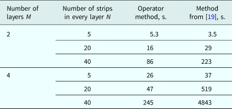
Comparison of computation time of the presented method and method from [Reference Kaliberda, Lytvynenko and Pogarsky19] is given in Table 1. Remarkable efficiency of the proposed method can be seen in the small computation time that is measured in few minutes. As we expected, with the number of scatterers increased, the operator method becomes more efficient. We also compare computation time with HFSS. Since for structures in Figs 3–5 it requires prohibitively large simulation times, we take two strips placed in parallel planes, M = 2, N = 1. HFSS requires about 20 hours.
Comparison of computation time

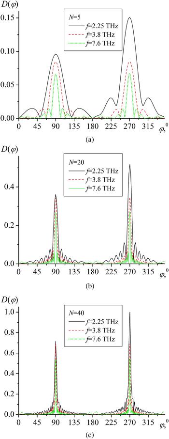
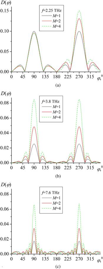
Figures 6 and 7 show the normalized scattering patterns of the far-field for three values of frequency: near the first plasmon resonance, f = 2.25 THz, and near the first and the second resonances of a layered structure, f ≈ 3.8 THz, and f ≈ 7.6 THz. As it is usual for strip gratings, if the number of strips increases, the number of side lobes increases, the main lobe level increases, and its width decreases. The levels of the main lobes of the reflected and transmitted fields are almost the same except for the first plasmon resonance frequency, f = 2.25 THz. Figure 7 is plotted to compare scattering patterns for different number of layers. Insignificant difference in the magnitude of the field reflected back to the source is observed for the structures which consist of one, two, and four layers only near the first plasmon resonance (Fig. 7(a)). For other frequencies, if the number of layers increases, the level of main lobe also increases.
Diffraction patterns for (a) N = 5, (b) N = 20, and (c) N = 40, f = 2.25 THz (solid curves), f = 3.8 THz (dashed curves), and f = 7.6 THz (dotted curves), M = 4 layers, μ c = 0.3 eV, τ = 1 ps, T = 300 K, d = 10 μm, h = l = 40 μm.

Diffraction patterns for (a) f = 2.25 THz, (b) f = 3.8 THz, and (c) f = 7.6 THz, M = 1 (dotted curves), M = 2 (dashed curves), and M = 4 (solid curves), N = 5, μ c = 0.3 eV, τ = 1 ps, T = 300 K, d = 10 μm, h = l = 40 μm.

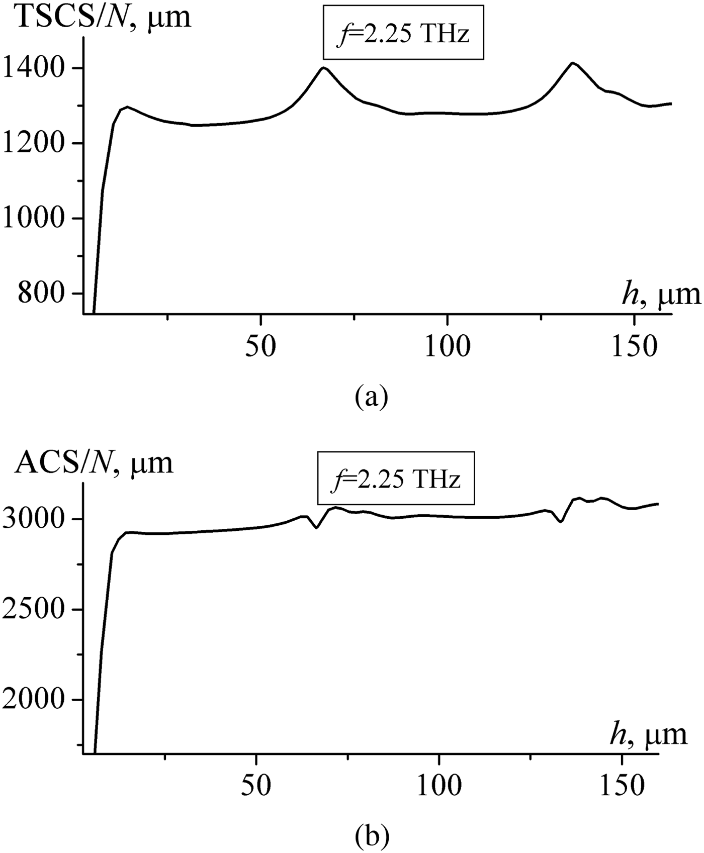
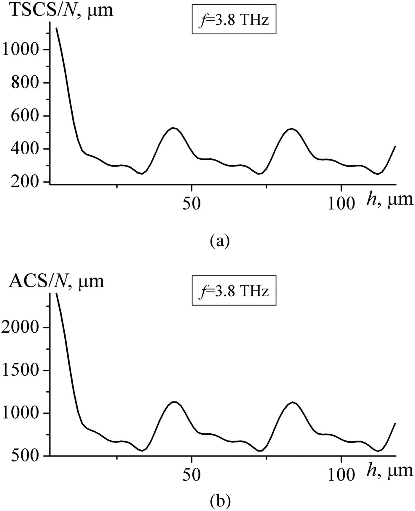
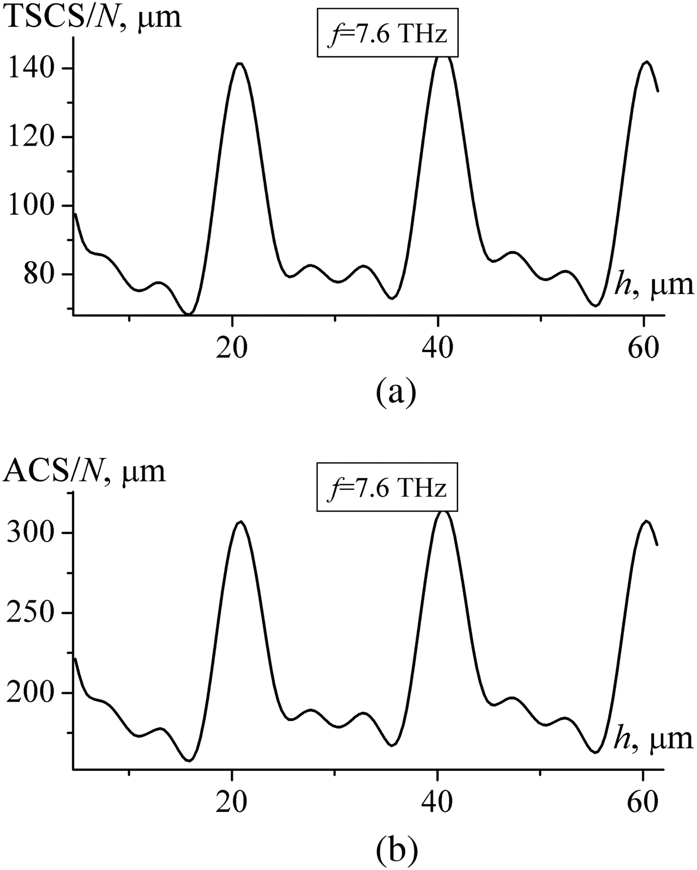
Figures 8–10 show dependences of TSCS and ACS versus distance between the layers. As we expected, the dependences are almost periodic with period kh ≈ 2π. Significant difference in dependences is observed for kh ≪ 1. It is explained by the strong interaction between the layers and partially reveals the influence of the evanescent waves.
Dependences of (a) TSCS and (b) ACS on the distance between layers h for f = 2.25 THz, M = 4, N = 20, μ c = 0.3 eV, τ = 1 ps, T = 300 K, d = 10 μm, l = 40 μm. Note the resonances related to the natural modes excited between the layers.

Same study as in Fig. 8 but for f = 3.8 THz.


Conclusion
We have presented efficient and rigorous analysis of the H-polarized wave diffraction by a finite multilayer graphene strip grating. Proposed approach allows to obtain the solution in several steps. At the first step, the scattering operators of a single layer should be determined. Then, the properties of the whole structure are obtained from the operator equations, which are equivalent to the Fredholm integral equations of the second kind. Such procedure allows to reduce the dimension of the matrix of the resulting system of equations.
We have studied TSCS, ACS, and far-field scattering patterns. Presented dependences demonstrate the resonances of a layered structure besides the plasmon resonances and Rayleigh anomalies.
 Mstislav E. Kaliberda received the B.S. and M.S. degrees in Applied Mathematics from the V.N.Karazin Kharkiv National University, Kharkiv, Ukraine in 2005 and 2006, respectively, and the Ph.D. degree in 2013 from the same university. Now he is an Associate Professor in the School of Radio Physics. His current research interests are the analytical and numerical techniques, integral equation, multi-element periodic structures, graphene gratings.
 Leonid M. Lytvynenko graduated from the V.N.Karazin Kharkiv National University, Kharkiv, Ukraine and received the combined B.S. and M.S. degree in Radiophysics and Electronics in 1959 and the Ph.D degree in 1965. From 1966 to 1985, he was with the Institute of Radiophysics and Electronics of the National Academy of Sciences of Ukraine (IRE NASU) in Kharkiv, Ukraine. He is a Professor in Radiophysics since 1977. In 1985, he founded the Institute of Radio Astronomy of NASU and served as its Director till 2017. His area of research is in the theory of waves scattering and propagation, antennas systems and engineering, microwave sources, and radio astronomy. He is the Vice-Chairman of the Ukrainian National URSI Committee, member of the European Astronomy Society, and member of the International Astronomy Society. He is also the Editor-in-Chief of the journal “Radio Physics and Radio Astronomy”.
 Sergey A. Poragsky received the M.S. degree in Radiophysics and Electronics from the V.N.Karazin Kharkiv National University, Kharkiv, Ukraine in 1977, and the Ph.D. degree from the same university in 1984. Since 1977 he has been with the same university as a researcher, and since 1984 as senior researcher and part-time senior lecturer at the Department of Physics of Ultra High Frequencies. Since 1999, he is a Professor, and part-time Principal Scientist. His research interests include CAD techniques for microwave and millimeter wave components, antenna systems, and microwave transmission lines and circuits.
 Mariia P. Roiuk is the B.S. student in Radiophysics of the V.N. Karazin Kharkiv National University, Kharkiv, Ukraine. Her research interests are in the scattering of waves by strip gratings.