1. INTRODUCTION
The increase in traffic in urban areas has been linked to a growing number of accidents and fatalities globally. In 2012, the total number of casualties in road accidents in the United Kingdom was 195,723, of which 1,754 were fatal and 23,039 were serious injuries (Kilbey, Reference Kilbey2013). Driving behaviour (including sudden lane change and erratic driving due to drowsiness) contributes to more than 90% of these accidents (Aljaafresh, Reference Aljaafresh2012). These driving styles, which might be characterised as weaving, swerving and jerky driving constitute irregular driving. Early detection of irregular driving within the lane has the potential to prevent the occurrence of accidents. Intelligent Transport Systems (ITS) technologies, with the function of providing the evaluation of driving performance and improvement of driving behaviours, can be used for irregular driving identification. Based on the lane level irregular driving identification technologies, more applications can be developed, such as lane control, collision avoidance and automatic driving. These applications could be used by vehicle manufacturers, logistic companies, police stations and other related departments. Previous research focusing on irregular driving identification in the early stages has mainly been based on two approaches, namely, the vehicle's real-time driving pattern detection and driver's physical behaviour monitoring.
For real-time driving pattern detection, various sensors, such as positioning, orientation, velocity and vision, are used to detect vehicle motion information, and the collected data are subsequently analysed to find cues of irregular driving. Lecce and Calabrese (Reference Lecce and Calabrese2008) proposed a system based on position and acceleration collection from the Global Positioning System (GPS) and accelerator, and used pattern matching to identify and classify driving styles. Chang et al. (Reference Chang, Hsu, Wang and Yang2008) developed a vision-based system with the function of learning the trajectories and longitudinal and lateral velocities of the vehicle and then used fuzzy neural network-based image processing information to identify the danger level of the vehicle. Krajewski et al. (Reference Krajewski, Sommer, Trutschel, Edwards and Golz2009) designed an orientation sensor-based system to collect driver fatigue information and used signal processing to capture fatigue impaired driving patterns. Dai et al. (Reference Dai, Teng, Bai, Shen and Xuan2010) proposed a system to detect dangerous driving based on the mobile phone with an accelerometer and orientation sensor. The warning will be issued if collected accelerations are matched with typical drunk driving patterns. Sultani and Choi (Reference Sultani and Choi2010) proposed a vision sensor-based approach for detecting and localising irregular traffic using an intelligent driver model. The image information was then learned using a neuron network to detect the abnormal driving. Mohamad et al. (Reference Mohamad, Ali and Ismail2011) used GPS to collect the position and velocity of the vehicle for the detection of abnormal driving. Imkamon et al. (Reference Imkamon, Saensom, Tangamchit and Pongpaibool2008) proposed a vision and orientation sensor-based method to collect driving information and then use fuzzy logic systems to classify different levels of hazardous driving. Although the real-time driving pattern detection approach has shown its great potential for irregular driving detections, a technical barrier that needs to be surmounted is the performance of vision sensor-based research that can be affected under various weather conditions. In addition, some research employing this approach significantly relies on the readings of high grade GPS or other motion sensors, the cost of which may hinder their wider practical use. Moreover, most of the above-discussed irregular driving detection systems are still in an early stage of development with neither field tests nor a robust algorithm to distinguish different types of irregular driving styles; therefore, their efficiency and reliability need to be further examined.
On the other hand, for driver physical behaviour monitoring, visual or auxiliary systems are always used. Visual observation is an option for detecting driver fatigue. Eriksson and Papanikolopoulos (Reference Eriksson and Papanikolopoulos2001) developed a vision-based system to monitor driver eyelid movement, where a warning would be triggered when irregular eye closure was observed. Zhu and Ji (Reference Zhu and Ji2004) developed a dual camera-based system on the dashboard to capture the visual cues of drivers, such as eyelid movement, gaze movement, head movement and facial expression. A probabilistic model was also developed to analyse the obtained fatigue information. Lee et al. (Reference Lee, Li, Liu, Chen, Chang and Lie2006) designed a camera-based system to capture the driver's sight line and driving path, and calculated their correlations to monitor the driving status and patterns. Albu et al. (Reference Albu, Widsten, Wang, Lan and Mah2008) used a vision sensor in conjunction with a force sensor on the accelerator pedal to monitor eye conditions and to collect the exerted force respectively, for driver fatigue monitoring. Omidyeganeh et al. (Reference Omidyeganeh, Javadtalab and Shirmohammadi2011) presented a vision sensor-based system to collect driver's eye closure and yawning information for drowsiness monitoring. Apart from the above research, auxiliary systems integrated with the vehicle for vehicle-driver interactions detection is also an option for monitoring the driver. Heitmann et al. (Reference Heitmann, Cuttkuhn, Aguirre, Trutschel and Moore-Ede2001) proposed various technologies, including a head position sensor, an eye-gaze system, a two pupil-based system and an in-seat vibration system for driver fatigue monitoring. Desai et al. (Reference Desai and Haque2006) proposed a system to define the level of drivers' alertness based on the time derivative of force exerted at the vehicle-human interface, such as pressure on the accelerator pedal. Sandberg et al. (Reference Sandberg, Akerstedt, Anund, Kecklund and Wahde2011) presented a method for abnormal driving detection by using physiological signals, such as signs of sleepiness detected by analysing brain activity through electroencephalography. Other auxiliary systems such as electrocardiogram, electromyogram, and skin conductance have also been investigated for the detection of driver fatigue and drowsiness (Mohamad et al., Reference Mohamad, Ali and Ismail2011). While driver physical behaviour monitoring has emerged as a promising approach, the vision sensor installed inside the vehicle can lead to a safety hazard due to driver distractions. Moreover, ambiguous road marks and bad weather can seriously affect the performance of the vision sensor. For the auxiliary system, compatibility issues can be raised as a coupled system is strictly required for system operation. Furthermore, the complexity and high cost of the auxiliary systems can make it difficult to integrate in practice. Thus, driver physical monitoring based on an irregular driving detection approach is difficult for wider application.
From the issues discussed above, this paper proposes a new lane level irregular driving identification algorithm based on a real-time driving pattern detection approach. The algorithm includes two parts. The first part is a GPS/INS integration algorithm to provide lane level positioning and high accuracy dynamic parameter estimation and the second part is a Fuzzy Inference System (FIS)-based irregular driving identification algorithm to distinguish different types of irregular driving. The proposed method takes advantage of merging high accuracy vehicle positioning and dynamic parameter estimations with different types of irregular driving identification technology, which has not been considered by previous investigations. Moreover, in this paper, for the initial field test, the outputs from the fusion algorithm for a Real Time Kinematic (RTK) GPS receiver and commercial INS are used for lane level irregular driving identifications without the need of vision or other high grade sensors. Using this method, the cost can be decreased and the results can be more environmentally insensitive. In the following discussions, Section 2 describes the GPS/INS integrated model with precise positioning and dynamic parameter estimation as well as the detection of driving events that characterise different types of driving styles based on FIS using estimated integrated results. Section 3 presents the test results and Section 4 concludes the paper.
2. IRREGULAR DRIVING DETECTION
The system is designed to link high precision positioning estimation with irregular driving detection. The improvement of vehicle positioning and dynamic parameters estimation accuracy is achieved by integrating precise vehicle models with GPS/INS-based positioning measurement and then using this in tandem with an irregular driving detection algorithm to recognise different types of irregular driving patterns.
2.1. System Overview
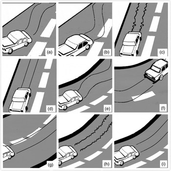
The specific irregular driving scenarios are generated on both straight and curved lanes. On the straight lane, the most common irregular driving styles for highways are weaving, swerving and jerky driving. On the curved lane, weaving and jerky driving can also occur, but swerving takes the form of over-turning or under-turning. Figure 1 presents the different types of driving styles, as elaborated in this paper.
Driving Styles: (a) Scenario 1 Weaving on Straight. (b) Scenario 2 Swerving on Straight. (c) Scenario 3 Jerky Driving on Straight. (d) Scenario 4 Normal Driving on Straight. (e) Scenario 5 Weaving on Curve. (f) Scenario 6a Over-turning on Curve. (g) Scenario 6b Under-turning on Curve. (h) Scenario 7 Jerky Driving on Curve. (i) Scenario 8 Normal Driving on Curve. (NHTSA, 2012)

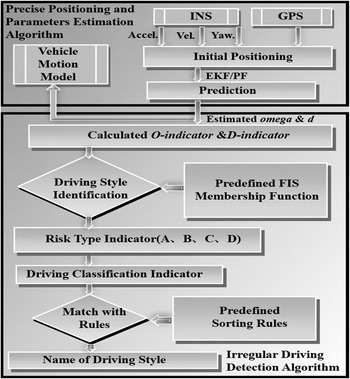
Based on the defined scenarios, omega and d, which are the vehicle's yaw rate and lateral displacement respectively, represent the vehicle's manoeuvres. In order to smooth the noises of the filter estimated values and extract the trend of their changes, Moving Average Deviation (MAD) of omega and d, noted as O-indicator and D-indicator respectively are developed to represent the different vehicle driving types. The system to detect irregular driving has to recognise a driving event that characterises the different driving styles based on the O-indicator and D-indicator derived from the filter estimated omega and d at every time epoch.
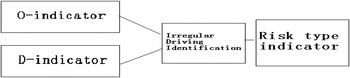
The framework of the system in Figure 2 shows the designed lane level irregular driving detection system, which contains two main parts. The first part is lane level precise positioning and parameter estimation algorithm. In order to collect the vehicle's driving data, one INS with one gyro and one accelerometer mounted along the vehicle body axis is used to output the yaw rate, acceleration and heading angle for the vehicle heading direction. One GPS is used to collect the vehicle's local coordinates and heading velocity. The collected initial position is used to feed the Particle Filter (PF) or Extended Kalman Filter (EKF) models with the precise vehicle motion models to provide the estimated positioning and attitude parameters for the next time epoch for iteration. The second part is the irregular driving detection algorithm. This started from the calculation of O-indicator and D-indicator based on the first part's estimated omega and d. These two indicators are then used as the input of the FIS for driving pattern identification. The FIS outputs the risk type indicator, which is defined with four fuzzy values A, B, C, D. The risk type level increases from A to D. Fuzzy value A means lowest risk type and D means highest risk type. In order to amplify the features of each driving style, driving classification indicators are then developed based on the risk type indicators. Finally, by comparison of the sorting of calculated driving classification indicator with predefined sorting rules of driving classification indicators extracted from the reference data, the system will output the identified driving style types, including weaving, swerving, jerky driving and normal driving on straight and curved lanes.
Framework of the Designed Irregular Driving Detection System.

2.2. Lane Level Positioning Design
The filter model design algorithm is critical for the estimated positioning performance, which is the key part of the lane level irregular driving detection system. PF and EKF are the most relevant and applicable filters for sensor integration; the design of the filter models based on PF and EKF are discussed in the following sub-sections.
2.2.1. Particle Filter Model-Based Design
The PF is a non-parametric implementation of a recursive Bayes filter. The probability density is approximated by a number N of weighted samples. Gustafsson et al. (Reference Gustafsson, Gunnarsson, Bergman, Forssell, Jansson, Karlsson and Nordlund.2002) presented the steps for the particle filtering process.
In the lane level precise positioning algorithm developed in this paper, the steps are described as follows:
2.2.1.1. Initialisation
The defined state vector is given by:
 $$X\left( t \right) = \left[ {xyv\theta {\rm \omega} a\beta d} \right]^T $$
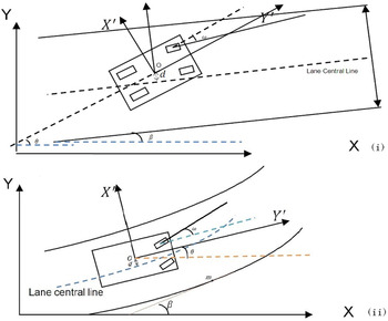
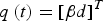
Where x is the X-axis coordinate (in metres) of the vehicle's geometric centre in the local UK National Grid coordinate system, y is the Y-axis coordinate (in metres) of the vehicle's geometric centre in the local UK National Grid coordinate system, v is the velocity at the heading direction, θ is the heading angle of the vehicle, ω is the vehicle yaw rate, a is the vehicle acceleration along the heading, β is the angle of inclination between the central line of lane segment and the X-axis of local British National Grid coordinates and d is the vehicle lateral displacement.
The state vector from Equation (1) can be divided into two sub state vectors. The stated vector Equation (2) is defined as the vehicle motion vector, which is for the particle filter cycle, and state vector Equation (3) is defined as the lane related vector, which is the dependent vector of state vector Equation (2) in the calculation.
 $$p\left( t \right) = [xyv\theta \omega a]^T $$
 $$q\left( t \right) = [\beta d]^T $$
In the particle filter operation, the parameters change with time epochs and particles with each parameter within the state vector Equation (1) expressed as
 $$X_t^i \; \left( {t = 0 \ldots n;i = 1 \ldots n} \right)\; $$
Where X ti is the parameters within the state vector Equation (1) at the time epoch t with the particle number i.
The filter begins with the initialisation of the particles x 0i of the vehicle motion vector p(t). To realise this, first the local coordinate sub-state variables x and y are randomly generated following a Gaussian distribution with the first accepted GNSS point as the mean value and a standard deviation value according to the GNSS a posteriori solution statistics. The initial heading velocity  $v_0^i$ is set as 0, for the initial position of the vehicle is assumed as static. Since it is assumed that no information on the initial heading is available, the values of θ are uniformly spread through the whole range of 2π space and the initial ω 0i is 0.
For the initialisation of q(t), in the straight road section, β is a constant, while in the curved road section  $\beta _0^i \; $ depends on [x 0i,y 0i].
 $\beta _0^i$ is the corresponding angle within the local coordinates frame of the lane centre line.
 $d_0^i$is the minimum distance between [x 0i,y 0i] and the lane central line. The coordinates of the points on the lane central line are stored as the database for calculation of β and d. In this paper, during the simulation, the coordinates of the points on the lane central line are defined based on the PTV Vissim software. PTV Vissim software allows the user to generate the lane information and simulate the traffic pattern exactly. More details of Vissim can be found on the PTV website (PTV, 2014). During the field test, the coordinates of the points on the lane central line are surveyed by high grade INS. β is calculated by the arctangent of the X-axis dividing by Y-axis of the points on the central line. d is calculated based on the following two steps. First, searching for the nearest two points on the central line from the vehicle's location. Second, calculating the length of the perpendicular line to the straight line containing these two points.
2.2.1.2. Filter Prediction
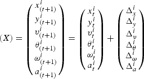
The prediction of p(t) is calculated as follows:
 $$(X) = \left( {\matrix{ {x^i _{(t + 1)}} \cr {y^i _{(t + 1)}} \cr {v^i _{(t + 1)}} \cr {\theta ^i _{(t + 1)}} \cr {\omega ^i _{(t + 1)}} \cr {a^i _{(t + 1)}} \cr}} \right) = \left( {\matrix{ {x^i _t} \cr {y^i _t} \cr {v^i _t} \cr {\theta ^i _t} \cr {\omega ^i _t} \cr {a^i _t} \cr}} \right) + \left( {\matrix{ {\Delta ^i _x} \cr {\Delta ^i _y} \cr {\Delta ^i _v} \cr {\Delta ^i _\theta} \cr {\Delta ^i _\omega} \cr {\Delta ^i _a} }} \right)$$
 $\Delta _x^i , \Delta _y^i, \Delta _v^i, \Delta _\theta ^i, \Delta _\omega ^i \Delta _a^i \; $ are different for the different vehicle motion models. In this paper, Constant Velocity (CV) and Constant Acceleration (CA) models are applied on the straight highway motion. The CV and CA are linear motion models with the assumption of a constant velocity or a constant acceleration in the timescale of the vehicle motion. Constant Turn Rate and Acceleration (CTRA) and Constant Turn Rate and Velocity (CTRV) models are applied in the curved scenarios. CTRV model assumes that the movement of the objects is tracked by the system at a constant turn rate and constant velocity and CTRA model assumes that the speed is changing at a constant rate, which is the tangential acceleration, while the object's turn rate also remains constant over time. These motion models have performed reasonable approximation of motions by vehicles on highways treating straights and curves separately (Tsogas et al., Reference Tsogas, Polychronopoulos and Amditis2005).
From the geometry relationship of the lane segment in Figure 3, the prediction of q(t) can be expressed as:
 $$\beta _{t + 1}^i \approx \beta _t^i $$
 $$d_{t + 1}^i = d_t^i + sin \left( {\beta _t^i} \right)\Delta _x^i - cos \left( {\beta _t^i} \right)\Delta _y^i $$
Geometry Relationship Between Vehicle and Lane on a Straight Lane (i) and Curved Lane (ii).

2.2.1.3. Filter update
The prediction cycle is applied at every input sample. First, the judgment of di is made. The valid di should comply with the equation |di| < 3HL where 3HL is three times half of the lane width (i.e. 1·5 times of the lane width). The reason for specifically considering 3HL as an indicative limit is that in reality, it is impossible for a vehicle to move from the current lane to a non-adjacent lane within 0·1s. Assuming a lane width of 3·5 m, if |di| is larger than 3HL = 5·25 m, which indicates the predicted position of the particle is in the non-adjacent lane, which is non realistic. So this particle is considered to be a measurement error (Toledo-Moreo, Reference Toledo-Moreo, Bétaille and Peyret2010).
If di is within this interval, the prediction parameters of t + 1 are calculated. However, these predictions are only considered as valid when the position predicted for a particle i is still within the bounds of the lane width. Therefore, after every prediction phase, the condition given by the following equation must be verified as below.
If |d t+1i| < 3HL is satisfied and the predicted d t+1i is accepted, then the other predicted parameters are accepted. If |d t+1i| < 3HL is not satisfied, the other predicted parameters are considered as invalid and the weighting of the particle is thus set as ${\rm \;} w_0^i = 0$. GNSS validity is tested after every prediction cycle and used to adjust the predicted particles to output the particle filter estimates.
2.2.1.4. Normalisation and resampling
After every update phase, the weights of the particles are modified, and the normalisation and resample test phases of a PF is relaunched.
2.2.2. Extended Kalman Filter Model-Based Design
The Extended Kalman Filter (EKF) is similar to the Kalman Filter (KF), but can be used in non-linear systems because it linearizes the transformations via the Taylor Expansion. In the EKF, a linear function is not required for the state transition and observation models of the state as it is instead comprised of differentiable functions (Mohinder and Angus, Reference Mohinder and Angus2008). There are two steps in the EKF process: correction and prediction. In the correction step, the error covariance is computed as it is minimised by the Kalman gain factor. The measurement data are applied to correct state estimation by adding the product of the Kalman gain and the prediction error to the prediction. In the prediction step, the next state is predicted by the current state variables using the system model (Barrios et al., Reference Barrios, Himberg, Motai and Sadek2006).
For the system developed in this paper, the state vector, consisting of six parameters, is:
 $$x\left( t \right) = \left( {xyv\beta \; \theta \; \omega } \right)^T $$
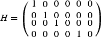
The measurement space only includes parameters of location, velocity and angle rate.
The measurement vector is:
 $$ z\left( t \right) = \left( {xyv\omega} \right)^T $$
The relationship between z and x is:
 $$ z\left( t \right) = Hx\left( t \right)$$
H is the Jacobian of the measurement model:
 $$H = \left( {\matrix{ {1} \cr 0 \cr {\matrix{ 0 \cr 0}} } \matrix{ {0} \cr {1} \cr {\matrix{ 0 \cr 0 }} } \matrix{ {0} \cr {0} \cr {\matrix{ {1} \cr {0} }} } \matrix{ {0} \cr {0} \cr {\matrix{ {0} \cr {0}}} } \matrix{ 0 \cr 0 \cr {\matrix{ 0 \cr 1}} } \matrix{ {0} \cr {0} \cr {\matrix{ 0 \cr 0 }} } } \right)$$
After correcting the previously predicted values, the system is ready to predict the next position by using the state vector equations. For the four vehicle motion models (CV, CA, CTRV, CTRA), each one has its own EKF model. For every prediction, d is calculated to be the minimum distance between [x, y] and the lane central line.
2.3. Irregular Driving Identification
The Fuzzy Inference System (FIS) is a widely used pattern matching method for detecting driver behaviour. The FIS is an inference system that maps input to output using fuzzy logic through combination rules (Aljaafresh et al., Reference Aljaafreh, Alshabatat and Najim Al-Din2012). Compared to traditional logic theory, where binary sets have two values: true or false, fuzzy logic variables define a truth value that ranges in degree between 0 and 1. Fuzzy logic extended to deal with the concept of partial truth, where the truth value is ranging between completely true and completely false. Fuzzy logic inference is a simple approach to solving problems instead of attempting to model it mathematically, which results in the FIS depending on human experience more than the technical understanding of the problem (Lecce and Calabrese, Reference Lecce and Calabrese2008). The fuzzy inference system consists of three stages: fuzzification, fuzzy inference and defuzzification to classify the different risk levels of each manoeuvre. For each designed irregular driving style, the different sorting of the driving classification indicator values can represent different driving styles. In order to pick up the features, the FIS is applied to the O-indicator and D-indicator data to get values for the risk type indicators.
Based on the output of the risk type indicator values for every time epoch, the total risk type indicator numbers in defined risk types are calculated followed by the driving classification indicator. The sorting rules extracted from driving classification indicators from the reference data is applied to the integrated model estimated driving classification indicator data to judge the driving types.
3. SIMULATION AND INITIAL FIELD TEST
The estimated positioning accuracy using both PF/EKF with motion models on straight and curved lanes are compared. The estimated outputs from different fusion models for irregular driving detection are compared and analysed. The tests presented in this paper are carried out with Matlab and Simulink and the lane data for scenarios are created by the PTV Vissim software.
3.1. Simulation Data Generation
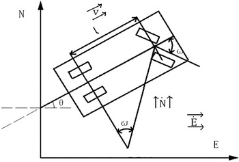
The scenarios are generated based on the extracted true driving styles on straight roads and curved roads. The designed lane width is set as 3·5 m since it is the regularised lane width of both highways and city roads. Two types of trajectories are generated. The first is the simulated reference trajectory, which is recognised as ‘true’ trajectory. It is generated based on a velocity 85–120 km/h with lateral displacements ranging from 0–1·25 m. A simple vehicle kinematic model is used to generate the trajectory of the vehicle and the related data for the simulation, see Figure 4 and Equations (12) – (14). The model takes into account the vehicle's velocity, heading and yaw rate. Using the yaw rate and lateral displacement as input, the vehicle's easting and northing coordinates can be determined (Clanton et al., Reference Clanton, Bevly and Hodel2009).
Geometry of the simple vehicle kinematic model.

The simple equations are
 $$\dot E = vsin\left( \theta \right)$$
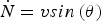 $$\dot N = vsin\left( \theta \right)$$
 $$\theta = \displaystyle{v \over l}{\rm tan}\left( \omega \right)$$
Where E is the easting coordinates of the vehicle in UK National Grid coordinates, N is the northing coordinates of the vehicle in UK National Grid coordinates, E˙ is the easting velocity of the vehicle, N˙ is the northing velocity of the vehicle, v is the heading velocity of the vehicle, θ is the heading angle of the vehicle, ω is the yaw rate and l is the vehicle wheelbase.
For the straight scenarios, the simulated reference trajectories are designed to drive along the X-axis to make the calculation simpler. As X-axis is assumed to be the Easting direction and Y-axis is assumed to be the Northing direction, only Northing coordinates are considered, and therefore only lateral position is considered. For the generation of the trajectory of Scenario 1, the kinematic motion model in Equations (12) – (14) is used. In addition, an amplitude sinusoidal yaw rate is used to generate a slow oscillation within the lane. Scenario 2 involves adding a sudden large yaw rate and then decreasing the lateral displacement gradually and back sharply. Scenario 3 is generated by very quick change of the yaw rate and lateral displacement input of the kinematic motion model. Scenario 4 is generated with the yaw rate and lateral displacement with very small amount of noise added. The reference data for the curved scenarios are generated based on the curved lane generated by PTV Vissim software. Scenario 5 is generated with the sinusoidal amplitude added following the curved lane. Over-turning and under-turning in Scenario 6 has been generated by sudden large or small yaw rates and then keeping similar heading angle to the lane curvature. Scenario 7 for jerky driving on a curve has been generated based on a quick change of yaw rate and lateral displacement input of the kinematic motion model and with a constant yaw rate to follow the curved lane. Scenario 8 for normal driving on the curve is generated on a constant small yaw rate and very small lateral displacement with a small amount of noise added.
The second type of data is simulated GPS and INS for the predefined scenarios. High accuracy positioning-related results are a basic requirement for the systems to identify irregular driving. The data for the vehicle positioning and dynamics are 10 Hz frequency data with the mean accuracy of 0·8 m, generated by the Spirent GPS simulator and simulated INS sensor data from Matlab for the predefined scenario routes.
3.2. Scenarios Positioning Results
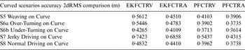
There are two filters (EKF and PF) and four motion models (CV, CA, CTRV and CTRA). Therefore, for the straight lane, the combination of fusion model can be EKFCV, EKFCA, PFCV and PFCA. For the curved lane, the combination of fusion model can be EKFCTRV, EKFCTRA, PFCTRV and PFCTRA. The accuracy 2dRMS between the generated reference position and fusion model estimated position for the straight and curved scenarios are shown in Table 1 and Table 2.
Accuracy Comparison of Model Estimated Results for Straight Scenarios.

Accuracy Comparison of Model Estimated Results for Curved Scenarios.

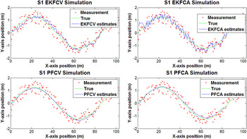
From the simulation results in Table 1 and Table 2, all of the fusion models provide decimetre positioning accuracy in both straight and curved scenarios based on the current filter settings. The initial measurement noise for EKF is set as 0·8 m and the initialisation setting for PF is with a 0·8 m standard deviation value for 1000 generated initial particles, according to the GPS a posteriori solution statistics. By comparing the positioning results from EKFCV, EKFCA, PFCV and PFCA model estimations, in general, the EKF filters produce more noise, while the PF filter estimations are comparatively smooth, see Figure 5 as an example for the integrated estimation positioning results for Scenario 1.
Integrated Estimation Positioning Results for S1.

3.3. Judgment Rules Extraction
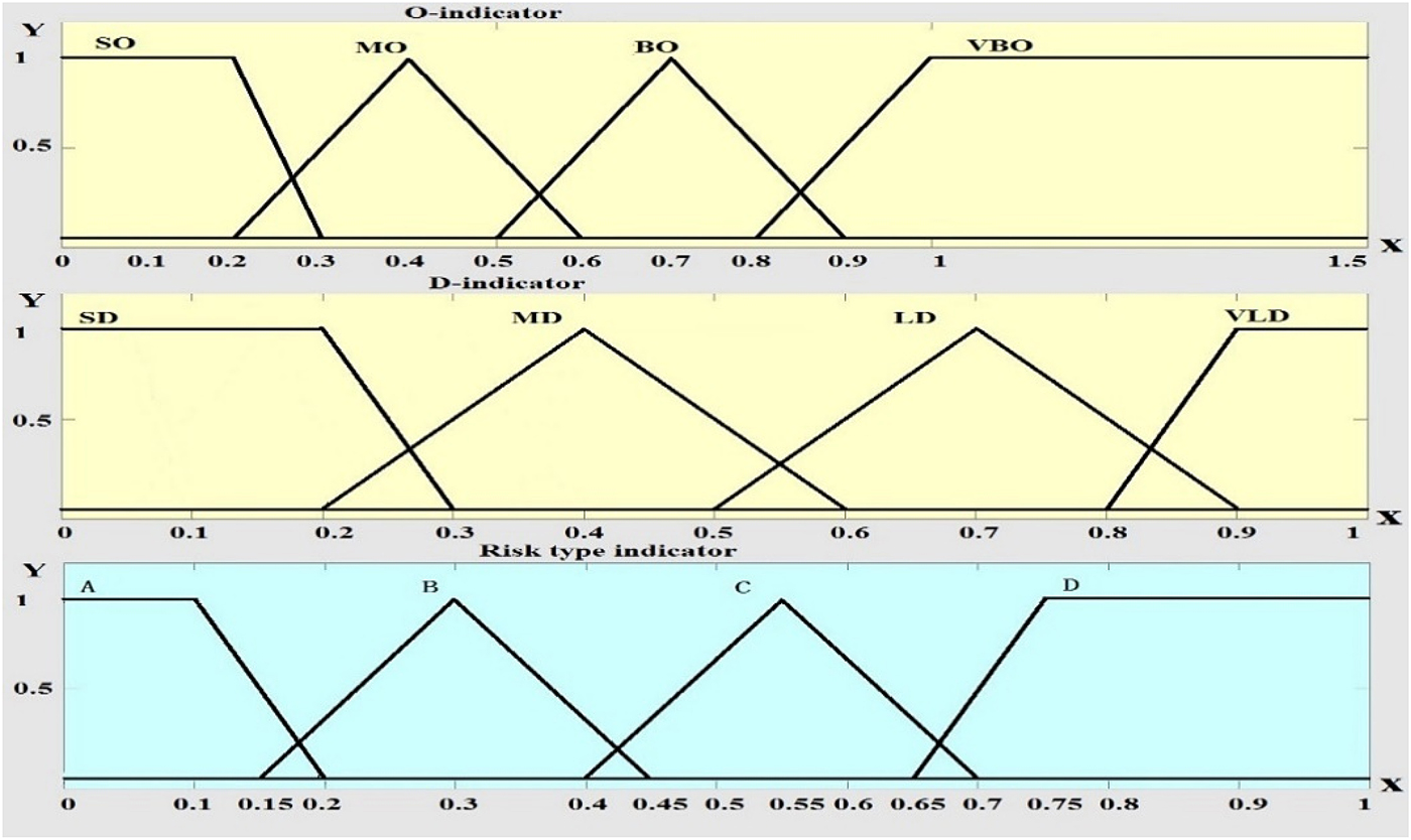
The O-indicator and D-indicator estimated from the fusion model are the input of the FIS system to calculate the risk type indicator for each fusion model. Figure 6 shows the structure of the fuzzy inference system.
Fuzzy Inference System Structure.

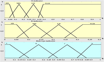
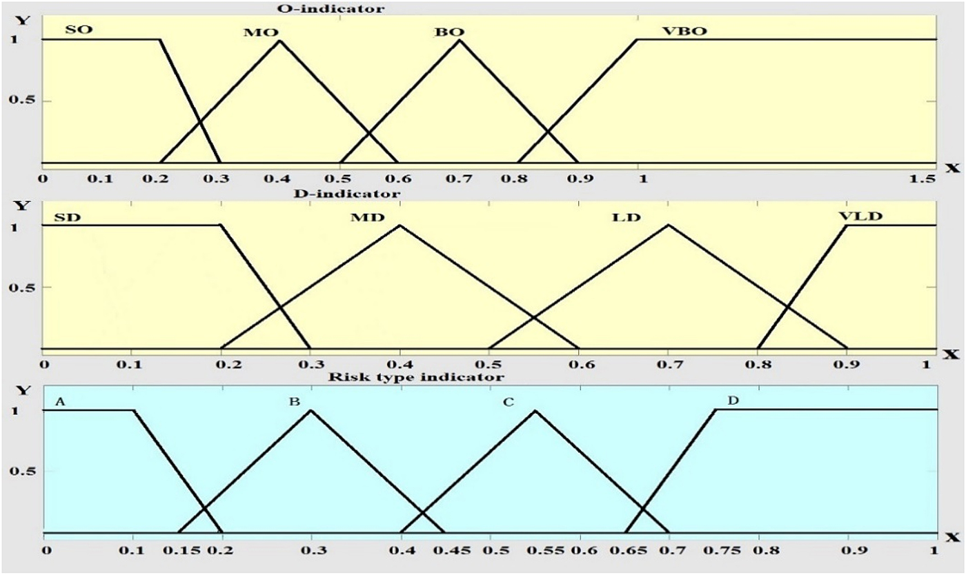
The designed membership function for the O-indicator and D-indicator values and risk type indicator in straight and curved scenarios are shown in Figure 7 and Figure 8, respectively. The fuzzy values defined in the membership functions are based on the experience data. In Figure 7 and 8, the first input is O-indicator data and corresponding fuzzy values in FIS are defined as Small O-indicator (SO), Medium O-indicator (MO), Large O-indicator (LO), and Very Large O-indicator (VLO). The membership functions for the SO and VLO fuzzy sets are a trapezoidal function, the triangular function is used for MO and BO. The second input is the D-indicator and the corresponding fuzzy values are defined as Small D-indicator (SD), Medium D-indicator (MD), Large D-indicator (LD), and Very Large D-indicator (VLD). Finally, the output of the system is the driving risk type indicator, which is defined by four fuzzy values A, B, C, D. The membership functions for A and D fuzzy sets are trapezoidal function and the triangular function for B and C.
Membership Function for the Straight Scenarios.

Membership Function for the Curved Scenarios.
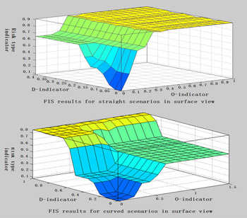
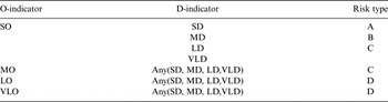
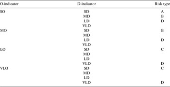
Tables 3 and 4 show the rules for the straight and curved scenarios defined based on the experience data. Figure 9 shows the designed FIS results in surface view, which presents the one pair of O-indicator value and D-indicator value as having one corresponding risk type indicator value.
Designed FIS Results in Surface View.

Rules of FIS for Straight Scenarios.

Rules of FIS for Curved Scenarios.

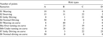
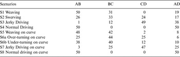
Based on the risk type indicator output of the FIS, the points in each risk type for all the scenarios during the last 5 s are collected and calculated in Simulink. The reason for using the back 5 s data as the time interval is that 5 s duration contains a total of 50 sets of data and is sufficient to provide information for the FIS judgement of the driving style (Chang et al., Reference Chang, Hsu, Wang and Yang2008). Table 5 shows the statistics of the number of points in each risk type calculated from the reference data. It can be seen that each scenario returns one or two dominant risk types in the 5 seconds sample. If there was only one dominant risk type for a given scenario containing the most points, it would be straightforward to classify the scenarios. However, this is not always the case with two or more risk types having a similar number of points for some scenarios. For example, in S7, there are two dominant risk types with 25 points in risk type D and 22 points in risk type C. In order to amplify the features of each scenario, the points in relevant risk types are combined as shown in Table 6, effectively resulting in a new driving classification indicator for the classification of driving styles.
Statistic of Number of Points in Risk Types for Reference Data.

Driving Classification Indicators for Reference Data.

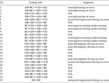
The four parameters in the driving classification indicator are developed based on the sum number of points in relevant risk types, e.g., AB is the sum number of risk type A and risk type B; BC is the sum number of risk type B and risk type C; CD is the sum number of risk type C and risk type D; AD is the sum number of risk type A and D. Based on the calculation and comparison results of the AB, BC, CD and AD parameters in Table 6, the sorting rules can be extracted to represent the feature of each scenario. For example, AB>BC>CD>AD is extracted as the rule for weaving from S1. Thus, the rules for detecting the features of each scenario are extracted in Table 7.
Sorting Rules for Driving Style Judgment.

The sensitivity test has been carried out to test whether the extracted rules for the irregular driving detection algorithm can continuously detect different types of irregular driving. Availability and correct detection rate are two parameters developed to evaluate the performance of the irregular driving detection algorithm. Availability is the percentage of the available driving style detection output. Correct detection rate is the percentage of the correct driving style judgement output. The sensitivity test shows that the irregular driving detection algorithm can continuously identify the different driving styles and it also indicates that the availability and correct detection rate are related to the system output rate. If the system output rate is higher, the correct detection rate and availability rate will decrease. Thus, choosing a proper output rate for a required situation is critical.
3.4. Simulation Results Analysis
The driving classification indicators for straight scenarios are calculated based on the EKFCV, EKFCA, PFCV and PFCA models. By comparison of the sorting results with the reference, only PFCV and PFCA can correctly detect the driving styles in straight scenarios. Tables 8 and 9 show the driving classification indicators for the PFCV and PFCA estimations, respectively. In Table 8, it is indicated that the sorting rule is AB>BC>AD>CD for S1, which is identified as weaving. For S2, BC>CD>AB>AD, is identified as swerving. For S3, CD>AD>BC>AB, is identified as jerky driving. For S4, AB>AD>BC>CD, is identified as normal driving. The results show that the PFCV model results lead to the correct identification of the features for all the straight lane scenarios. Similar to PFCV, in Table 9, the PFCA-based identification is successful in all the straight lane scenarios. AB>BC>AD>CD is identified as weaving in S1. BC>CD>AB>AD is identified as swerving in S2. CD>AD>BC>AB is identified as jerky driving in S3. AB>AD>BC>CD is identified as normal driving in S4.
Driving Classification Indicators for Straight Scenarios Based on PFCV.

Driving Classification Indicators for Straight Scenarios Based on PFCA.

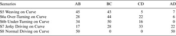
For the curved scenarios, all of the models have made misdetections except the PFCTRA model. As it is shown in Table 10, the PFCTRA model can offer good estimations, where the values in driving classification indicators are closest to the driving classification indicators output from the reference data.
Driving Classification Indicators for Curved Scenarios Based on PFCTRA.

In summary, for the classification of the driving types in simulation, both of the EKFCV and EKFCTRV models have wrongly detected swerving/under-turning as jerky driving or weaving. Both of the EKFCA and EKFCTRA models have wrongly detected weaving/weaving on curve as swerving/swerving on curve. Furthermore, EKFCTRA also wrongly detects normal driving as weaving on a curve. The PFCV model can detect the driving styles on straights correctly, while the PFCTRV model incorrectly detects swerving on curve as weaving on curve. Both of the PFCA and PFCTRA models have correctly detected the different driving features separately. They have the smallest error in positioning and correctly detected the scenarios on straights and curves separately. In the next section, the initial field test is carried out based on the PFCA/PFCTRA model estimations on highways.
3.5. Initial Field Test
The initial field test is to validate the lane level irregular driving detection algorithm. The test includes two issues to be validated. The first issue is to validate the FIS-based irregular driving detection algorithm and the second issue is to validate lane level precise positioning algorithm in the designed field session.
The data for the initial field test were collected via a seven minute duration journey on the M4 motorway near Ravenscourt Park, United Kingdom. During the journey, one jerky driving manoeuvre carried out from 15:51:41·5 to 15:51:59·2 on the curved lane is defined as Session 1. The vehicle was driven at speeds ranging from 70 km/h to 120 km/h and the data were collected at a frequency of 10 Hz. The specifics of the equipment used in the experiment were as follows.
• Leica Viva GNSS GS15 RTK GPS receiver for GPS data collection, including the position and speed of the vehicle.
• I-Mar RT-200 INS for real-time attitude data collection, including heading angle and yaw rate of the vehicle. The sensor also has the function of outputting GPS/INS combined measurements, which are post-processed by forward and backward processing for a high accuracy reference.
For validation of the FIS-based irregular driving detection algorithm, the post-processed GPS/INS combined measurements are directly input into the irregular driving detection algorithm to output the results. The output rate is chosen with 1 Hz, 5 Hz and 10 Hz. The output driving classification indicator for Session 1 shows CD>BC>AD>AB, which is in accordance with the jerky driving style. Table 11 shows the first detection time epoch for Session 1 on various output frequencies from the reference results. The reference data-based field test results show the jerky driving on a curve can be detected on the routes. It also indicates that the higher the output rate, the earlier the detection time epoch, which is identical to the simulation results.
The First Detection Time Epoch of Session 1 Based on the Reference Results with Respect to Different Output Frequencies.

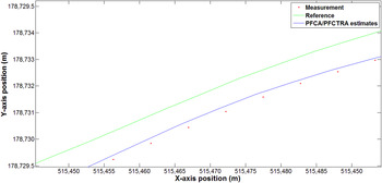
For the validation of the lane level precise positioning algorithm, the GPS measurements output from the Leica Viva GNSS GS15 RTK GPS receiver are fed to the PFCA/PFCTRA model for positioning and dynamic parameter estimation and then the estimated results are used for the FIS-based irregular driving detection algorithm. A typical RTK fixed ambiguity solution accuracy is a few centimetres, however, from the output of the positioning solutions, it is shown that only 84·04 % of total collected measurements are determined with the RTK fixed ambiguity solution on the route. There are still some types of low quality positioning solutions, such as a Differential GPS solution and float ambiguity solution. Thus, only sub-metre mean positioning accuracy can be achieved from the GPS measurements. From the calculation results, the PFCA/PFCTRA model estimated positioning solutions have significantly improved the positioning accuracy compared to original collected measurements, which indicate that the mean positioning accuracy in the route is reduced to 0·6214 m from 0·9664 m, especially the mean accuracy for Session 1 is reduced to 0·382 m from 0·569 m. Figure 10 shows a comparison of collected measurement positions and PFCA/PFCTRA estimated positioning results with respect to reference. It is clear that PFCA/PFCTRA estimated results are closer to the reference than the measurements.
Comparison of Measurement and PFCA/PFCTRA Estimated Positioning Results with Respect to Reference.

The sorting of parameters in driving classification indicator based on the PFCA/PFCTRA model estimated results output CD>BC>AD>AB for Session 1, which is detected as jerky driving on a curve. The first detection epoch of Session 1 based on the PFCA/PFCTRA estimated results in Table 12 performs similar results with the reference data, which means that the PFCA/PFCTRA estimated results are capable of identifying the defined session.
The First Detection Epoch of Session 1 Based on the PFCA/PFCTRA Estimated Results with Respect to Different Output Frequencies.

The comparison of the availability and correct detection rate of the irregular driving detection algorithm for both reference and PFCA/PFCTRA estimated results with respect to the output rate for Session 1 is shown in Table 13. Obviously, the availability and correct detection rate decrease as the output rate increases, which is identical to the simulation. The availability and correct detection rate based on the PFCA/PFCTRA estimated results are lower than that from the reference results, as the PFCA/PFCTRA estimations have more errors than the reference.
The Comparison of Availability and Correct Detection Rate from the PFCA/PFCTRA Estimated Results and Reference Results with Respect to Different Output Rates for Session 1.

4. CONCLUSIONS
A novel lane level irregular driving identification algorithm is presented in this paper. This study exploits an integrated sensor fusion algorithm for precise position and parameter estimation and then uses a FIS-based irregular driving identification algorithm to provide precise lane level irregular driving identification. The performance of the algorithms developed in this paper is tested based on simulated irregular driving data and an initial field test.
In the simulation, two types of data are generated based on the defined scenarios (weaving/weaving on curve, swerving/over/under turning, jerky driving/jerky driving on curve and normal/normal on curve). The first type of data is reference data, for the definition of scenarios and the extraction of the sorting rules from the driving classification indicator for further irregular driving detection. From the sensitivity analysis of the irregular driving detection algorithm based on the reference data, it can be observed that a higher output frequency of the irregular driving detection could lead to an earlier initial detection time of the specific driving style. In addition, the availability and correct detection rate will decrease with the increase of the output rate of the system. The second type of data are the simulated GPS and INS measurements data, which are used to test the designed precise positioning algorithms and the irregular driving detection results. From the performance of the positioning accuracy of the designed integration model for the simulated GPS and INS measurements, the PF model exhibits a less significant error than the EKF model and the CA model exhibits less significant error than the CV model during the simulation. The PFCA and PFCTRA models show the highest positioning accuracy in their scenarios separately. In addition, as the PFCV, PFCA and PFCTRA models have the higher estimation accuracy, only these three model-based estimations have correctly distinguished the different irregular driving scenarios.
The initial field test has validated that FIS-based irregular driving detection algorithm is feasible, and PFCA/PFCTRA filter estimated results can improve the accuracy of collected GPS measurements and detect the defined irregular driving session. Future work will involve collecting more field data in different sessions and evaluating the performance of the developed algorithm in different field situations.