2 Development of outflow instabilities and secondary reconnection

In order to study the properties of outflow instabilities and secondary reconnection, we use particle-in-cell numerical simulations.

We consider here the same run previously considered in Lapenta et al. (Reference Lapenta, Markidis, Goldman and Newman2015). The system is initialized with a Harris equilibrium (Harris Reference Harris1962)

uniquely specified by the mass ratio $m_{i}/m_{e}=256$ , the temperature ratio $T_{i}/T_{e}=5$ and $v_{th,e}/c=0.045$ . We set the density of the uniform plasma background to $n_{0b}=n_{0}/10$ , the value of the guide field to $B_{0z}/B_{0x}=1/10$ and the thickness of the initial current sheet to $\unicode[STIX]{x1D6FF}=0.5d_{i}$ . The evolution is followed using the fully electromagnetic and fully kinetic iPic3D code (Markidis, Lapenta & Rizwan-uddin Reference Markidis and Lapenta2010) that treats both electrons and ions as particles. Details are provided in Lapenta et al. (Reference Lapenta, Markidis, Goldman and Newman2015). We use coordinates where $x$ is along the initial magnetic field, $y$ is along the initial gradients and $z$ is along the initial current. Open boundary conditions are imposed in the $x$ and $y$ direction and periodicity is imposed along $z$ . We consider a three-dimensional box of shape $[40.0,15.0,10.0]d_{i}$ , where $d_{i}$ is the ion inertial length, which is resolved by a Cartesian grid of $[512,192,128]$ cells, each one populated with 125 particles. The spatial resolution is $\unicode[STIX]{x0394}x=1.25d_{e}$ , where $d_{e}$ is the electron inertial length, and the time step is $\unicode[STIX]{x0394}t=\unicode[STIX]{x03C0}/10\unicode[STIX]{x1D714}_{ce}^{-1}$ , where $\unicode[STIX]{x1D714}_{ce}$ is the electron gyro-frequency.

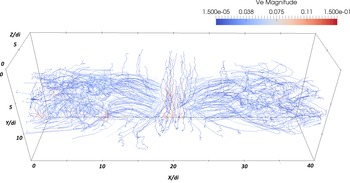
Reconnection is initialized in the centre with an initial $x$ -shaped perturbation that leads to the formation of a central $X$ -line. A reconnection site develops with plasma accelerated towards the reconnection region and expelled out of it. The electron flow pattern in the fully developed nonlinear stage is shown in figure 1. The electrons are first attracted toward the central $X$ -line where the $z$ -directed reconnection electric field accelerates them to high speed. The Lorentz force then deflects the particles towards the outflow. In this region, the system presents a remarkable invariance along $z$ , resembling the same physics of two-dimensional fast kinetic reconnection.

In the outflow, however, the electron flow pattern becomes distorted and meanders about, eventually passing downstream away of the reconnection region. In this region the electron flow becomes more turbulent.

Figure 1.

Visualization of the electron flow around a reconnection site. We report streamlines of the first-order moment of the electron distribution (the electron flow velocity) coloured by the intensity of the local electron speed (normalized to the speed of light).

The region of electron meandering corresponds to the front formed by the interaction of the outflowing plasma with the surrounding media. At the front, an effect similar to that of a snowplough pushes the plasma outward. A form forms where at least three of the mechanisms mentioned above are present: the field lines wrap around the front gaining unfavourble curvature that can lead to interchange-type instabilities, the density gradient is unstable to drift modes and the distribution function becomes severely non-Maxwellian leading to microinstabilities.

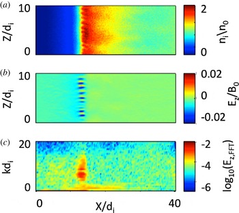
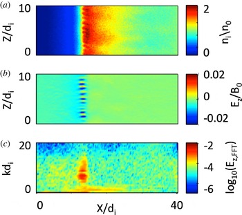
Figure 2 shows the state of the front after the instability starts to develop. The density (a) becomes rippled by a mode that presents a strong perturbation of the $E_{z}$ (b). When the mode structure of these fluctuations is Fourier analysed, the resulting spectrum in $k_{z}$ is reported in (c). The observed features are characteristic of a drift mode in the lower hybrid range.

Figure 2.

Early stages of the instability at the front, at time $\unicode[STIX]{x1D714}_{ci}^{-1}=15$ . The panels show from top to bottom: ion density (a), $z$ -component of the electric field (b) and the Fourier spectrum in $k_{z}$ of the perturbation of the electric field $E_{z}$ (c).

Figure 3.

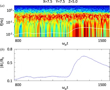
Signal from a virtual probe embedded in the simulation at $x/d_{i}=7.54$ , $y/d_{i}=7.54$ , $z/d_{i}=5.04$ . (a) Shows the spectrogram of the $E_{z}$ signal measured. To guide the eye the local lower hybrid frequency is indicated by a white line. (b) Shows the magnetic field intensity measured by the virtual probes at the different times.

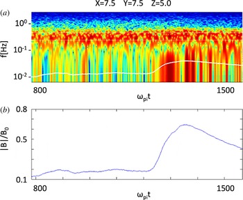
The identification of the instability as having primarily the nature of a lower hybrid drift instability (LHDI) is confirmed by the temporal spectrum measured at a fixed point reached by the front (Divin et al. Reference Divin, Khotyaintsev, Vaivads and André2015a ,Reference Divin, Khotyaintsev, Vaivads, André, Markidis and Lapenta b ). A spectrogram, obtained with standard windowing methods similar to those used on board real space probes, is reported in figure 3: the observed frequency spectrum is reported at different times. Panel (b) reports the corresponding observed local magnetic field intensity. When the front arrives, an intense signal in the lower hybrid range is measured.

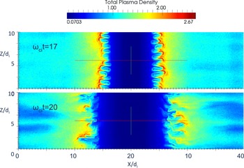
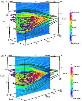
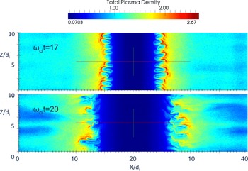
As the evolution is continued, the ripples in the front become more intense and start to interact leading to conditions where magnetic field of opposite polarity is brought in contact promoting secondary reconnection. Figure 4 shows the front at two consecutive times: at later times, the ‘fingers’ formed in the front tend to interact and coalesce (Vapirev et al. Reference Vapirev, Lapenta, Divin, Markidis, Henri, Goldman and Newman2013).

Figure 4.

Density at the front for two different times.

Lapenta et al. (Reference Lapenta, Markidis, Goldman and Newman2015) analysed several indicators to detect positively secondary reconnection sites: direct analysis of field line connectivity, energy conversion in the electron frame ( $\boldsymbol{J}\boldsymbol{\cdot }(\boldsymbol{E}+\boldsymbol{v}_{e}\times \boldsymbol{B})$ ), electron agyrotropy, slippage ( $\boldsymbol{v}_{e\bot }-\boldsymbol{E}\times \boldsymbol{B}/B^{2}$ ), topological measure of field line breakage (Hesse & Schindler Reference Hesse and Schindler1988; Biskamp Reference Biskamp2000) ( $\boldsymbol{b}\times \unicode[STIX]{x1D735}\times (E_{||}\boldsymbol{b})$ ), where $\boldsymbol{b}$ is the unit vector along $\boldsymbol{B}$ and $E_{||}$ is the parallel component of the non-ideal part of Ohm’s law (Biskamp Reference Biskamp2000), normalized as $eE_{||}/m_{i}c\unicode[STIX]{x1D714}_{pi}$ .

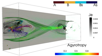
A specific orientation of the magnetic field which allows for the field annihilation and energy release, is an important indicator of magnetic reconnection. In the classical two-dimensional picture, magnetic field lines of opposite direction approach each other and form an $X$ -point, which, extended to three dimensions, becomes an $X$ -line denoted by the strong $Z$ -aligned current in our simulation. This sort of magnetic reconnection, however, does not require the field to become exactly zero (hence, no magnetic nulls are formed) on the reconnection site. We use the technique based on the topological degree method (Greene Reference Greene1992) as described in Olshevsky et al. (Reference Olshevsky, Deca, Divin, Peng, Markidis, Innocenti, Cazzola and Lapenta2016) to locate and classify magnetic nulls. Indeed, in the simulation reported here, no magnetic nulls are present in the central current sheet as summarized in figure 5. However, the diffusion region around the $X$ -line is characterized by strong electron agyrotropy $A=(P_{e,\bot 1}-P_{e,\bot 2})/P_{e,\bot 1}-(P_{e,\bot 2})$ that is shown with volume rendering. No strong energy conversion is associated with the ‘main’ reconnection $X$ -line.

Figure 5.

Combination of different measures at the same time: a vertical cut of the electron current intensity (grey scale); false colour volume rendering of agyrotropy; magnetic null points (coloured spheres) coloured according to their topological type. Selected field lines reconnected once at the primary site are shown in green, while secondary reconnected lines near the nulls are shown in purple, pink, orange and light blue.

In contrast, in the reconnection outflow a number of magnetic nulls form, which are depicted by coloured spheres in figure 5. The colour denotes the magnetic nulls’ topological type: A and B (red and orange) are the three-dimensional extensions of the $X$ -points called radial nulls; while As and Bs (light blue and blue) represent magnetic islands or magnetic flux ropes. Both radial and spiral nulls are present in the outflows, however the number of spiral ones is larger. Magnetic field lines in the vicinity of the null points in the left outflow are shown with the corresponding colours. A pair of spiral nulls is formed in a swirl of the light blue magnetic field lines, probably driven by a shear instability. This null pair is embedded in the region of strong energy conversion (see figure 5). Other nulls in this outflow are on the interfaces of magnetic fields of different polarities characterized by complex field patterns resembling an $X$ pattern (orange) and merging into flux ropes (purple and pink). Recent observations (Fu et al. Reference Fu, Vaivads, Khotyaintsev, André, Cao, Olshevsky, Eastwood and Retinò2017) provide a strong evidence that intermittent energy conversion in the reconnection outflows is associated with the spiral magnetic nulls and twisted magnetic fields.

The picture provides an indication of the scenario described in the introduction: the initial reconnection site located at the centre of the box and forming an $X$ -line produces two outflows that become unstable and produce in turn secondary reconnection sites. In the process the plasma becomes effectively turbulent and a large fraction of the energy is converted to particle heat at these unstable fronts, rather than at the central $X$ -line.

3 Development of intermittent turbulence in reconnection outflows

Above we have observed how reconnection tends to become visually turbulent. But is turbulence real? In a recent paper (Pucci et al. Reference Pucci, Servidio, Sorriso-Valvo, Olshevsky, Matthaeus, Malara, Goldman, Newman and Lapenta2017), the properties of electric and magnetic fluctuations that are produced by magnetic reconnection have been analysed. Because of the inhomogeneous background it is important to first establish the anisotropy level and in general the three-dimensional (3-D) properties of turbulence. Analysis of the autocorrelation function of the magnetic field fluctuations have shown that the turbulence that develops in the reconnection jets is anisotropic. In particular, magnetic vortexes are elongated in the direction of the background magnetic field, namely $x$ , with a second smaller anisotropy in the $(y,z)$ plane. The second anisotropy becomes negligible for smaller scales and isotropy is recovered in the $(k_{y},k_{z})$ plane for $k_{yz}>1.5$ , with $k_{yz}=\sqrt{k_{y}^{2}+k_{z}^{2}}$ . This allows us to reduce the 3-D spatial spectra to 1-D isotropic spectra computed in the $(k_{y},k_{z})$ plane and integrated in $k_{x}$ . The results of this computation shows magnetic and electric spectra with a clear power law in the sub-ion range $1.5<k_{yz}d_{i}<15$ . As observed in space plasmas (Eastwood et al. Reference Eastwood, Phan, Bale and Tjulin2009) the magnetic and electric spectra depart from each other at around $kd_{i}\sim 1$ , the electric one proceeding with a spectral slope of ${\sim}1$ and the magnetic one with a slope of $-8/3$ . Recently Matteini et al. (Reference Matteini, Alexandrova, Chen and Lacombe2017), following simple dimensional arguments, have interpreted this phenomenon as due to the dominance of the Hall effect at small scales. It is worth remarking how this interpretation still holds in such an anisotropic and inhomogeneous system, where spectra need to be carefully extracted removing large-scale background profiles and border effects.

Turbulence is responsible for the transfer of energy from fields to particles. In this work we show that this energy exchange does not take place homogeneously in the reconnection events but is located in small regions in the reconnection outflows where the energy transfer is very intense. In order to quantify the energy exchange we introduce the two dissipation proxies $D_{l}=\boldsymbol{J}\boldsymbol{\cdot }\boldsymbol{E}$ and $D_{i}=\boldsymbol{J}\boldsymbol{\cdot }(\boldsymbol{E}+\boldsymbol{v}_{i}\times \boldsymbol{B})$ (Zenitani et al. 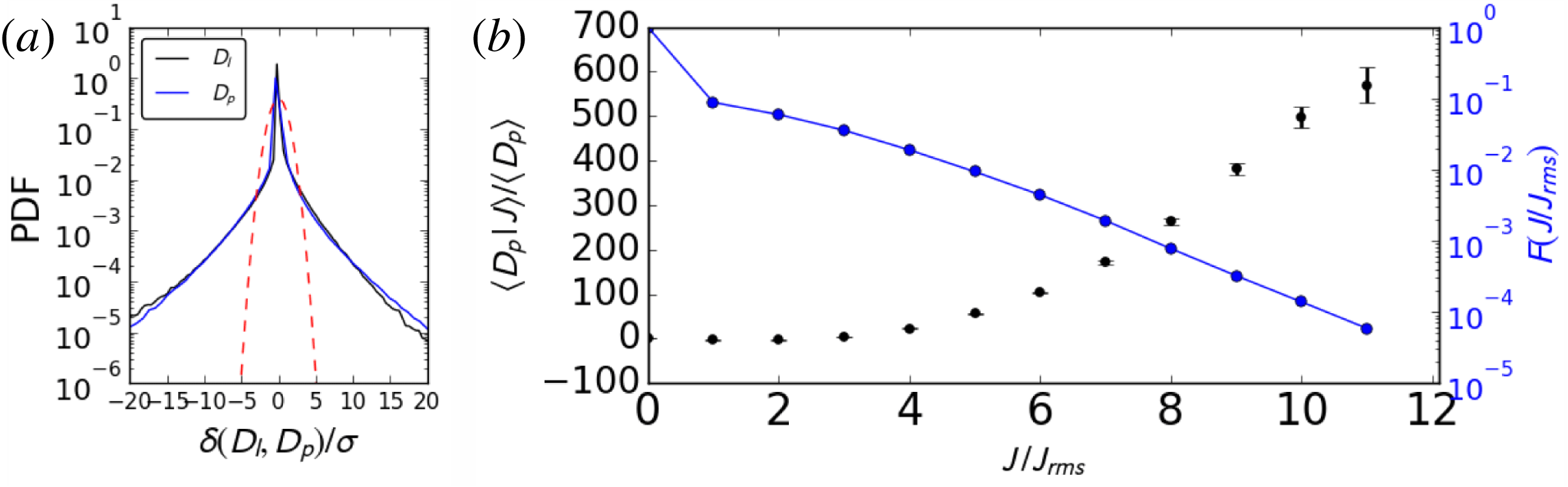Reference Zenitani, Hesse, Klimas and Kuznetsova2011), where $\boldsymbol{J}$ is the total current, $\boldsymbol{E}$ is the electric field, $\boldsymbol{v}_{i}$ is the ion fluid velocity and $\boldsymbol{B}$ is the magnetic field. In figure 7(a) the probability density functions (PDFs) of $\unicode[STIX]{x1D6FF}D_{l}=D_{l}-\langle D_{l}\rangle _{x,y,z}$ and $\unicode[STIX]{x1D6FF}D_{i}=D_{i}-\langle D_{i}\rangle _{x,y,z}$ are plotted, where $\langle ~\rangle _{x,y,z}$ means average along the three axes. The two PDFs are compared with the normalized Gaussian distribution (plotted with the dashed-red line). They strongly depart from Gaussian distributions, presenting instead high tails up to several standard deviations $\unicode[STIX]{x1D70E}$ . In (b), the average $D_{i}$ conditioned to a threshold current density is shown. The plot is constructed as follows: a threshold in the current density magnitude is considered and the average of $D_{i}$ is computed using all those points in the domain where the value of the current is bigger than the fixed threshold. This average is then normalized to the average of $D_{i}$ on all points, which gives by definition $\langle D_{i}|J=0\rangle /\langle D_{i}\rangle =1$ . The black points in the plots represent the result of such a computation for different values of the threshold. The blue curve represents the filling factors, i.e. the fraction of points used for computing the average with respect to the total number of points in the sample. The average of $D_{i}$ strongly increases when higher threshold are considered up to $J/J_{rms}=10$ , where $J_{rms}$ is the root of the mean square current. Our results confirm that the exchange of energy is local, with larger values of $D_{i}$ localized in very small volume filling structures. This evidence and the presence of non-Gaussian PDFs of the dissipation proxies suggest that magnetic reconnection produces small-scale current sheets which are the site of strong events of energy exchange between fields and particles. Concisely stated, all these statistics indicate that dissipation in a reconnection event is intermittent. A similar conclusion was reached by Wan et al. (Reference Wan, Matthaeus, Karimabadi, Roytershteyn, Shay, Wu, Daughton, Loring and Chapman2012) who examined the electron frame dissipation surrogate conditioned on the magnitude of the current density.

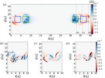
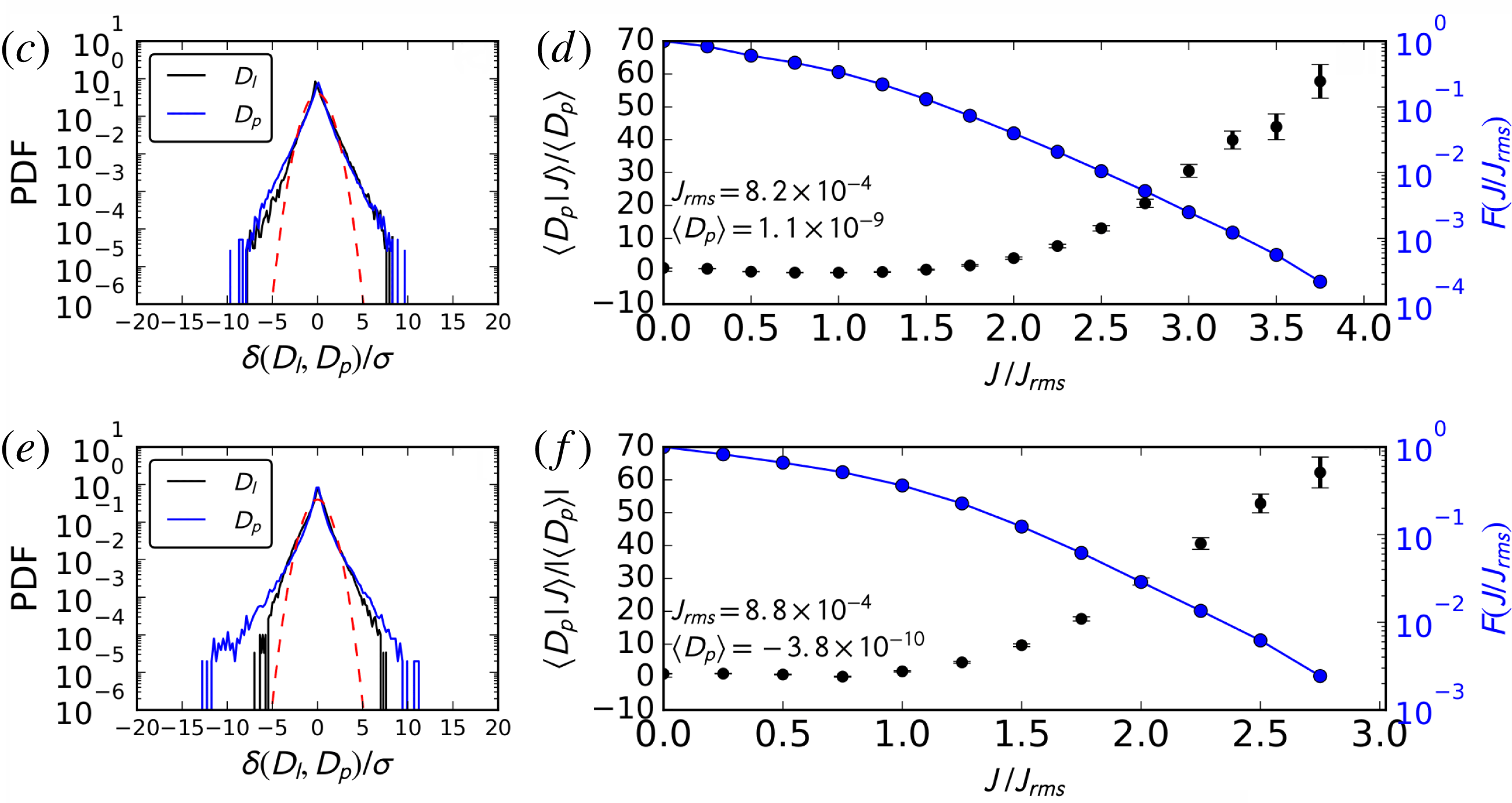
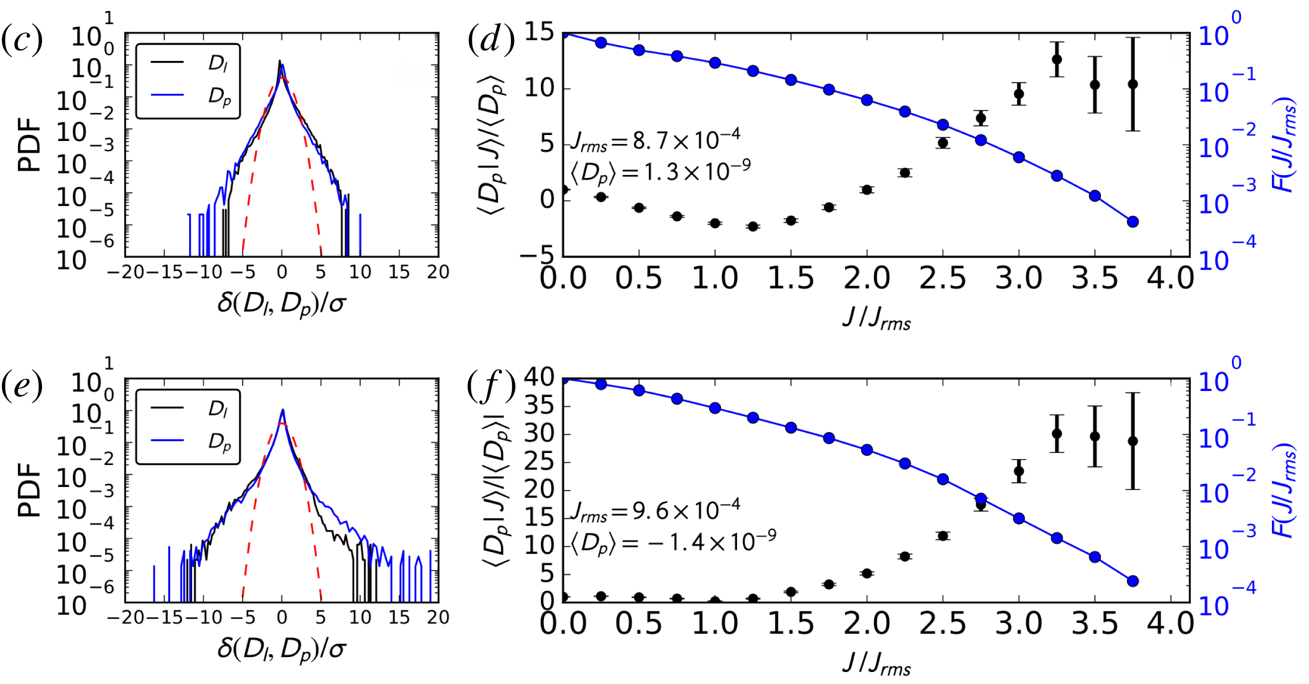
Figures 8 and 9 show the statistics of dissipation proxies presented in figure 7 computed in sub-boxes located in the two reconnection outflows (see figure 6). Non-Gaussian statistics and the increasing conditioned average of the dissipation proxies indicate that intermittent turbulence is at play in both reconnection outflows.

Figure 6.

Energy exchange $D_{l}=\boldsymbol{J}\boldsymbol{\cdot }\boldsymbol{E}$ in the $(x,y)$ plane averaged in the $z$ direction (a), and in the $(y,z)$ plane at $x=33\,d_{i}$ (b), $x=36\,d_{i}$ (c), $x=39\,d_{i}$ (d). The $X$ -line is located at $x=20\,d_{i}$ . The three boxes in (a) are the ones used for the statistical analysis presented in figure 8–9.

Figure 7.

PDFs of $D_{l}$ and $D_{i}$ (a). Red dashed lines represent the normalized Gaussian curve. Mean $D_{i}$ conditioned on local current density thresholds and (right axis) fraction $F$ of the full box data used to compute the averages (b).

Figure 8.

PDFs of $D_{l}$ and $D_{i}$ in $BOX_{1}$ (c), $BOX_{2}$ (e). Conditioned average of $D_{i}$ and filling factors $F$ in $BOX_{1}$ (d), $BOX_{2}$ (f) (left outflow).

Figure 9.

PDFs of $D_{l}$ and $D_{i}$ in $BOX_{3}$ (c), $BOX_{4}$ (e). Conditioned average of $D_{i}$ and filling factors $F$ in $BOX_{3}$ (d), $BOX_{4}$ (f) (right outflow).

4 Energy exchanges in reconnection outflows

As shown in figure 5, the region of the outflow is characterized by intense energy exchange ( $\boldsymbol{J}\boldsymbol{\cdot }\boldsymbol{E}$ ). Recently, the energy budget has been analysed in detail (Lapenta et al. Reference Lapenta, Goldman, Newman and Markidis2016b ) and a large fraction of the energy is deposited as particle energization, while a significant fraction is also transported by the Poynting flux.

Figure 10 reports the ion temperature at the end of the run. Ions are generally not magnetized in the reconnection region and projecting the pressure tensor in the parallel and perpendicular direction relative to the magnetic field is not productive. Ion energization in reconnection outflows and in reconnection fronts have been analysed in theory and in simulation (Aunai, Belmont & Smets Reference Aunai, Belmont and Smets2011; Pan et al. Reference Pan, Ashour-Abdalla, El-Alaoui, Walker and Goldstein2012; Birn et al. Reference Birn, Hesse, Nakamura and Zaharia2013; Lapenta et al. Reference Lapenta, Ashour-Abdalla, Walker and El Alaoui2016a ). Complex processes are at play, requiring a full analysis of the phase space and of single particle trajectories to detect with accuracy the specific mechanisms accelerating the particles (Eastwood et al. Reference Eastwood, Goldman, Hietala, Newman, Mistry and Lapenta2015).

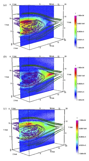
Figure 10 reports the three different kinetic temperatures obtained from the pressure tensor: $\unicode[STIX]{x1D61B}_{j}=P_{jj}/\unicode[STIX]{x1D70C}_{i}$ , for $j=x,y,z$ . The primary region of reconnection tends to heat the ions primarily in the $y$ direction. This effect is due to the mixing of the two populations of ions coming from above and below from the inflow towards the reconnection region. In the outflow, instead, the plasma outflowing along the $x$ -direction mixes with the plasma in the medium causing apparent heating in the $x$ -direction (Aunai et al. Reference Aunai, Belmont and Smets2011). Heating in the $z$ direction is present both in the region of primary reconnection, where it is due to the acceleration of non-magnetized ions in the reconnection region due to the reconnection electric field (Moses, Finn & Ling Reference Moses, Finn and Ling1993; Divin et al. Reference Divin, Markidis, Lapenta, Semenov, Erkaev and Biernat2010), and in the region of the outflows, where it is a consequence of the instabilities in the outflows. These effects however should not be interpreted as heating in the meaning of increasing thermodynamic temperature. The plasma is far from Maxwellian and what appears as heating in the kinetic temperature (i.e. the second-order moment of the distribution) is in reality the presence of multiple interpenetrating populations.

Figure 10.

Ion temperature in the outflow: from top to bottom: $T_{x}$ (a), $T_{y}$ (b) and $T_{z}$ (c). The left half of the domain is reported at the final time along with selected field lines.

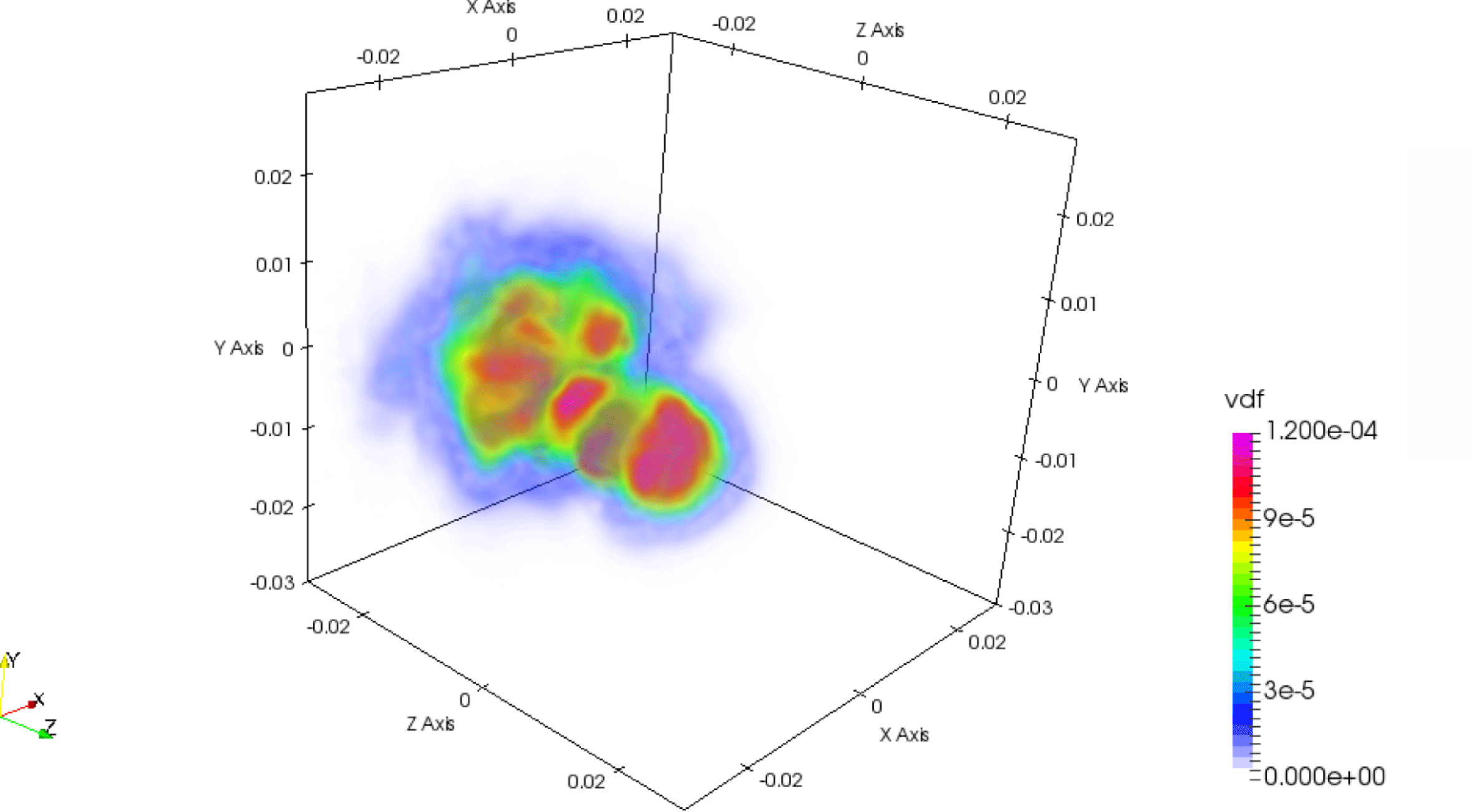
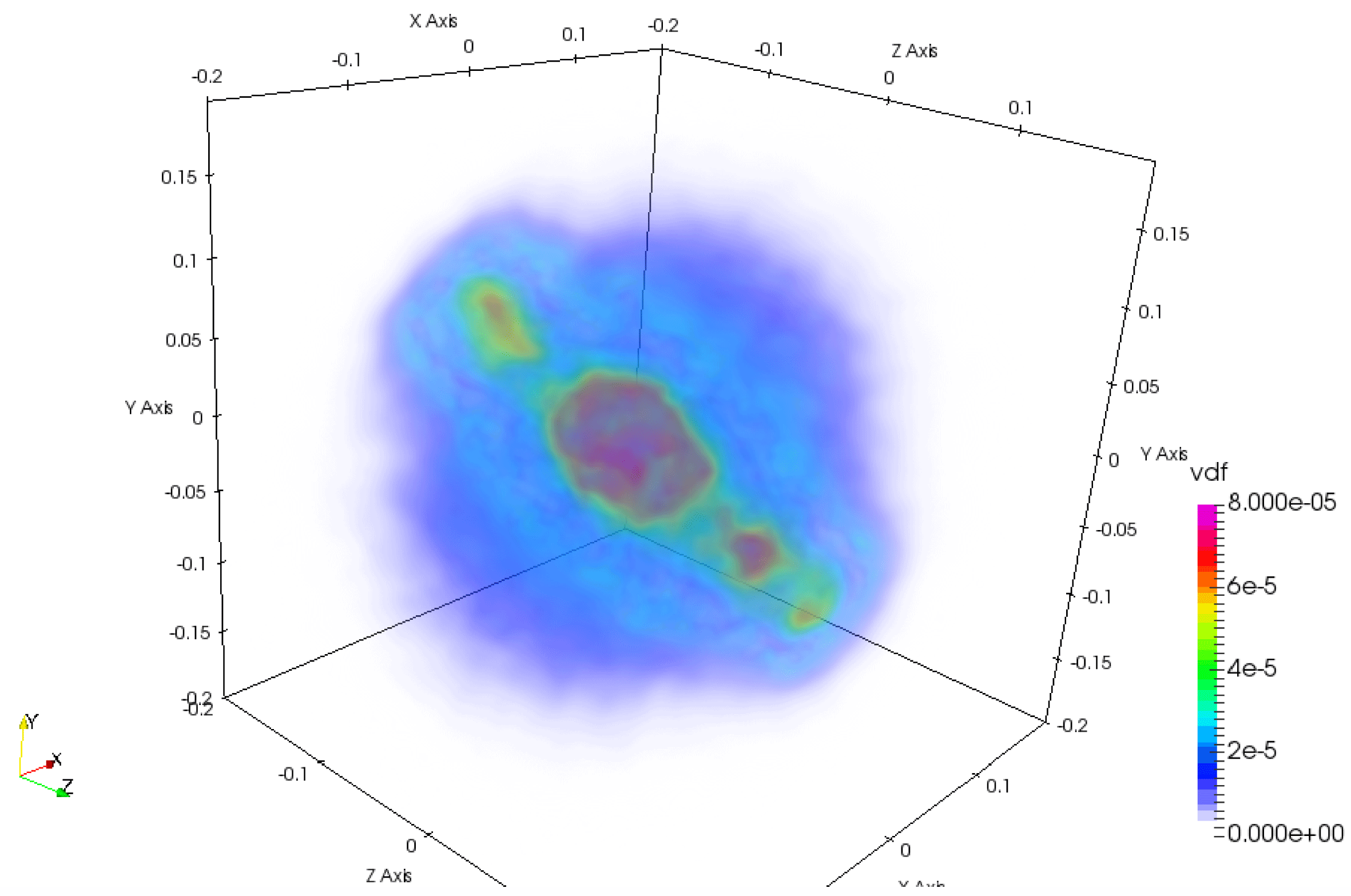
Figure 11 shows a volume rendering of the full 3-D velocity probability distribution for the ions. The distribution is anisotropic and contains multiple populations. When the second-order moment is taken to measure a kinetic temperature, the result can be misleading because multiple beams, each with its own temperature, appear as a single plasma with a combined temperature much higher than that of the beams. However, this is not a process of heating but one of bulk acceleration of ion populations. In a recent study, each ion component has been tracked back in time to its origin (Eastwood et al. Reference Eastwood, Goldman, Hietala, Newman, Mistry and Lapenta2015). Each component originates from different regions and their trajectories brought them to the same location but with different speeds.

Figure 11.

Volume rendering of the ion velocity probability distribution $f_{i}(v_{x},v_{y},v_{z})$ at the position $x/d_{i}=10.32$ , $y/d_{i}=7.5$ , $z/d_{i}=5$ , obtained by averaging over particles contained within a box centred at that location and with side $0.5d_{i}$ .

Similarly, figure 12 show the parallel and perpendicular electron temperature. The electrons are mostly magnetized and it is more convenient to report the electron temperatures in magnetic coordinates rather than along geometrical axes. The region of primary reconnection causes parallel heating (Ricci, Lapenta & Brackbill Reference Ricci, Lapenta and Brackbill2003). The cause is the reconnection electric field that accelerates the electrons along the $z$ direction (Wan et al. Reference Wan, Lapenta, Delzanno and Egedal2008; Divin et al. Reference Divin, Markidis, Lapenta, Semenov, Erkaev and Biernat2010): in this region the guide field is the only field present and the acceleration is parallel. The region of secondary instabilities in the outflow shows strong parallel and perpendicular energization caused by the conversion of electromagnetic energy (i.e. $\boldsymbol{J}_{e}\boldsymbol{\cdot }\boldsymbol{E}$ ) (Lapenta et al. Reference Lapenta, Goldman, Newman, Markidis and Divin2014a , Reference Lapenta, Goldman, Newman and Markidis2016b ).

Figure 12.

Electron parallel (a) and perpendicular (b) temperature in the outflow. The left half of the domain is reported at the final time along with selected field lines.

The electron distribution is typically far smoother than the ion distribution due to the higher thermal speed. However, in the region of the secondary front instability, even the electron distribution becomes complex. Figure 13 shows a volume rendering of the full 3-D velocity probability distribution for the electrons computed as described above for the ions. On a large scale the distribution is bi-Maxwellian with different parallel and perpendicular temperatures. Within it we can observe multiple electron populations caused by electron acceleration by the electric field, directed primarily in the directions $z$ (reconnection electric field) and $y$ (Hall electric field) (Wan & Lapenta Reference Wan and Lapenta2008). Acceleration is not present in the $x$ direction where in fact there are no strong macroscopic electric fields.

The magnetic field lines show a chaotic behaviour: this condition makes it possible for particles moving along chaotic filed lines to access new acceleration regions of space (Dahlin, Drake & Swisdak Reference Dahlin, Drake and Swisdak2017), possibly encountering multiple reconnection sites and increasing their energy in steps.

Figure 13.

Volume rendering of the electron velocity probability distribution $f_{e}(v_{x},v_{y},v_{z})$ at the position $x/d_{i}=10.32$ , $y/d_{i}=7.5$ , $z/d_{i}=5$ , obtained by averaging over particles contained within a box centred at that location and with side $0.5d_{i}$ .

5 Conclusions and future directions

The analysis of reconnection outflows in the present case of a weak guide field (1/10 of the main reconnecting field) show the development of an instability in the lower hybrid regime. In the present case, the instability has at least two components. The first, is due to the presence of density gradients formed in the pile-up region where the outflow meets the ambient plasma. The second is the pre-existing velocity shears due to the differential velocity between the Harris plasma and the ambient plasma (Lapenta, Brackbill & Daughton Reference Lapenta, Brackbill and Daughton2003; Karimabadi et al. Reference Karimabadi, Pritchett, Daughton and Krauss-Varban2003; Ricci et al. Reference Ricci, Brackbill, Daughton and Lapenta2004; Ricci, Lapenta & Brackbill Reference Ricci, Lapenta and Brackbill2004). The first instability leads to a Rayleigh–Taylor-type interchange instability in the lower hybrid range, while the latter leads to a kinking of the current layer.

Both instabilities feed the onset of a turbulent cascade with the presence of coherent structures and intermittency. The outflows becomes host to secondary reconnection sites where the magnetic field topology becomes chaotic (Lapenta et al. Reference Lapenta, Markidis, Goldman and Newman2015).

We investigate here the effect of these processes on the energization of particles. The ions and the electrons are energized not only in the primary reconnection site but also, and in some cases predominantly, in the reconnection outflows. Particle energization can be linked to the electric fields operating on the particles. Electric fields do not heat particles in the statistical meaning of increasing their thermal spread, rather they coherently energize all particles, creating beams. Beams originating from different regions interact and interpenetrate creating distribution functions with multiple populations.

The end result is that the second-order moment of the distribution is increased but the process cannot be interpreted as heating proper but rather as the presence of very non-Maxwellian distributions with multiple beams.