1 Introduction
Particle-laden turbulent flows are of fundamental importance in a great number of natural physical processes and in a host of industrial and environmental applications. Dust storms, pollutant dispersion, coal combustion, fluidized beds and pneumatic conveyance are only a few of the phenomena and applications in which particles play a significant role. In most turbulent flows laden with particles, modulation of turbulence is of particular interest. Despite several decades of extensive numerical and experimental investigation, however, the effects of inertial particles on turbulence modulation remain far from fully understood.
A great deal of experimental research on turbulence modulation by dispersed particles has been conducted during the past few decades. Tsuji, Morikawa & Shiomi (Reference Tsuji, Morikawa and Shiomi1984) used laser-Doppler velocimetry to measure both the air and the particle velocities with five different sizes of plastic particles in a vertical pipe flow. They found that large particles tended to augment the turbulence intensity, whereas small particles tended to attenuate it. In addition, medium-sized particles increased turbulence near the centre of the pipe but decreased it in the near-wall regions. Hetsroni (Reference Hetsroni1989) concluded that particles with lower Reynolds number suppressed turbulence, while particles with higher Reynolds number enhanced it owing to wake shedding behind the particles. Rashidi, Hetsroni & Banerjee (Reference Rashidi, Hetsroni and Banerjee1990) observed experimentally that larger polystyrene particles increased the number of wall ejections and thus augmented the turbulence intensity and Reynolds stress. Smaller particles, however, had the opposite effect. These effects increased with particle mass loading. Kulick, Fessler & Eaton (Reference Kulick, Fessler and Eaton1994) experimentally investigated particle–turbulence interactions in a downflow fully developed channel, and showed that the presence of small particles substantially attenuated the turbulence. Furthermore, the degree of attenuation increased with particle Stokes number, mass loading and distance from the wall. Hadinoto et al. (Reference Hadinoto, Jones, Yurteri and Curtis2005) studied experimentally the effect of fluid Reynolds number on turbulence modulation for a given particulate material and particle mass loading. Their results indicated that as the fluid Reynolds number increased, the fluid velocity fluctuations were enhanced while the particle velocity fluctuations were damped.
Since the 1990s, direct numerical simulation (DNS) has offered another approach to the investigation of turbulence modulation by particles. Squires & Eaton (Reference Squires and Eaton1990) and Boivin, Simonin & Squires (Reference Boivin, Simonin and Squires1998) performed DNS of particle-laden stationary homogeneous and isotropic turbulent flows with two-way coupling. They found that the viscous dissipation rate in the fluid decreased with increasing mass loading. However, viscous dissipation was slightly augmented in decaying isotropic turbulent flows laden with particles (Elghobashi & Truesdell Reference Elghobashi and Truesdell1993; Sundaram & Collins Reference Sundaram and Collins1999). Pan & Banerjee (Reference Pan and Banerjee1996) investigated the effects of near-neutral-density solid particles on turbulent open channel flow using DNS. They reported that particles smaller than the dissipative length scale caused an attenuation of the turbulence intensity and Reynolds stress, whereas larger particles enhanced both of these quantities. Vreman (Reference Vreman2007) numerically studied the turbulence characteristics in a vertical air–solid pipe flow and showed that the turbulence intensity, Reynolds stress and turbulence production decreased with increasing mass loading. Zhao, Andersson & Gillissen (Reference Zhao, Andersson and Gillissen2010, Reference Zhao, Andersson and Gillissen2013) observed pronounced turbulence modulation and drag reduction in a two-way coupled DNS of particle-laden channel flow. Particles with sufficiently large response times attenuated the Reynolds stress and the velocity fluctuations in the spanwise and wall-normal directions, but augmented the turbulence intensity in the streamwise direction. Gualtieri et al. (Reference Gualtieri, Picano, Sardina and Casciola2013) conducted a DNS of homogeneous shear flow seeded with small particles, focusing on particle clustering in the two-way coupling regime and on the turbulence modulation by particles. Their novel findings are of some significance for the modelling of turbulent multiphase flows. More recently, they have proposed a new method for capturing the interphase momentum exchange between the carrier fluid and the dispersed phase in a turbulent flow (Gualtieri et al. Reference Gualtieri, Picano, Sardina and Casciola2015).
According to these earlier studies, both attenuation and augmentation of fluid turbulence in the presence of inertial particles have been observed in laboratory experiments and numerical simulations. In general, small particles suppress the turbulence intensity, while larger ones enhance it. Based on the available data in the literature, several criteria have been proposed to predict the turbulence modulation caused by particles. Gore & Crowe (Reference Gore and Crowe1989) brought together the work of various investigators and proposed an intuitive parameter, the ratio of the particle diameter to the characteristic length of the most energetic eddy, to classify the enhancement or suppression of turbulence. However, a single classification cannot take account of the effects of other important parameters, such as particle Stokes number and mass loading, on turbulence modulation. Yarin & Hetsroni (Reference Yarin and Hetsroni1994) suggested that turbulence modulation is affected by four parameters: the particle mass loading, the ratio between particle and fluid densities, the particle Reynolds number and the ratio between particle diameter and a characteristic eddy diameter. Hadinoto et al. (Reference Hadinoto, Jones, Yurteri and Curtis2005) emphasized that for gas–solid flows, demarcation criteria based on gas and particle characteristic length scales (Gore & Crowe Reference Gore and Crowe1989) or on particle Reynolds number (Hetsroni Reference Hetsroni1989) are insufficient to predict turbulence modulation. Recently, Balachandar & Eaton (Reference Balachandar and Eaton2010) reviewed experimental and numerical studies of dispersed multiphase turbulent flows, and pointed out that the mechanisms of turbulence modulation and their parameter dependence were not well understood and remained topics for continuing fundamental investigation.
As is well known, near-wall turbulent flow is dominated by coherent structures, such as high- and low-speed streaks, sweep and ejection events, and quasi-streamwise vortices (Kline et al. Reference Kline, Reynolds, Schraub and Runstadler1967; Cantwell Reference Cantwell1981; Robinson Reference Robinson1991). Although the effect of near-wall turbulent coherent structures on particle behaviour has been the subject of many experiments and numerical simulations (Brooke et al. Reference Brooke, Kontomaris, Hanratty and McLaughlin1992; Kaftori, Hetsroni & Banerjee Reference Kaftori, Hetsroni and Banerjee1995; Rouson & Eaton Reference Rouson and Eaton2001; Marchioli & Soldati Reference Marchioli and Soldati2002; Sardina et al. Reference Sardina, Schlatter, Picano, Casciola, Brandt and Henningson2012), there is little research reported about the effect of inertial particles on coherent structures in the literature. Furthermore, the findings from these few research studies are not unanimous. Portela & Oliemans (Reference Portela and Oliemans2003) reported that the presence of particles led to strong damping of the intensity of streamwise vortices, although without any significant change in their shape and size. Dritselis & Vlachos (Reference Dritselis and Vlachos2008, Reference Dritselis and Vlachos2011) studied the effect of heavy solid particles on near-wall coherent structures in a vertical downward channel flow using an Eulerian–Lagrangian point-particle method. They found that the addition of particles increased the diameter and streamwise extent of the quasi-streamwise vortices. More recently, Li et al. (Reference Li, Wang, Liu, Chen and Zheng2012) experimentally investigated turbulence modulation in a dilute particle-laden channel flow. In addition to noticeable modifications of the mean velocity and turbulence intensity of the fluid, they also observed a remarkable reduction in the spatial scale of near-wall coherent structures due to the presence of particles.
Among these experimental and numerical studies, most have been devoted to isotropic turbulent flow or to parallel flows such as channel or pipe flows. However, little information is available about the effect of particles on a spatially developing flat-plate boundary layer. Rogers & Eaton (Reference Rogers and Eaton1991) were the first to measure particle–turbulence interaction in a vertical flat-plate boundary layer. They observed that the particles significantly suppressed the turbulence intensity. Furthermore, the suppression of the fluid turbulence seemed to be a strong function of the local particle concentration in the near-wall region. A later experimental study of the behaviour of particles in a horizontal boundary layer over a flat plate was carried out by Tanière, Oesterlé & Monnier (Reference Tanière, Oesterlé and Monnier1997). It should be pointed out here that, to date, there have been few reports of DNS of turbulence modulation in spatially developing turbulent boundary layers.
In spite of the numerous studies on particle-laden turbulent flows, turbulence modulation by small solid particles is still not completely understood, and many issues remain to be investigated. In particular, the interaction between particles and fluid turbulence in a zero-pressure-gradient flat-plate boundary layer remains an open question. Thus, it is of great significance to perform a two-way coupled DNS of a particle-laden turbulent boundary layer over a flat plate. To the best of our knowledge, this is the first attempt to investigate turbulence modulation in a flat-plate boundary layer by means of DNS. The main objective of the present work is to study the turbulence modulation and modification of near-wall coherent structures caused by particles in a flat-plate boundary layer by using an Eulerian–Lagrangian point-particle approach. The particle size is smaller than the Kolmogorov length scale. Three different simulations are performed to investigate the effects of particle characteristics, namely particle Stokes number and particle mass loading, on turbulence modulation.
2 Numerical method
2.1 Governing equations of fluid flow
In this study, the fluid is taken to be air with density
 $\unicode[STIX]{x1D70C}_{f}=1.205~\text{kg}~\text{m}^{-3}$
and kinematic viscosity
 $\unicode[STIX]{x1D708}=1.5\times 10^{-5}~\text{m}^{2}~\text{s}^{-1}$
. It is assumed that the flow is incompressible and Newtonian. The continuity and momentum equations for the fluid can be written in dimensionless form as
 $$\begin{eqnarray}\displaystyle & \displaystyle \unicode[STIX]{x1D735}\boldsymbol{\cdot }\boldsymbol{u}=0, & \displaystyle\end{eqnarray}$$
 $$\begin{eqnarray}\displaystyle & \displaystyle \frac{\unicode[STIX]{x2202}\boldsymbol{u}}{\unicode[STIX]{x2202}t}+\boldsymbol{u}\boldsymbol{\cdot }\unicode[STIX]{x1D735}\boldsymbol{u}=-\unicode[STIX]{x1D735}p+\frac{1}{Re_{\unicode[STIX]{x1D703}_{0}}}\unicode[STIX]{x1D6FB}^{2}\boldsymbol{u}+\boldsymbol{f}, & \displaystyle\end{eqnarray}$$
 $\boldsymbol{u}=(u,v,w)$
is the fluid velocity vector,
 $p$
is the fluctuating kinematic pressure,
 $Re_{\unicode[STIX]{x1D703}_{0}}=U_{\infty }\unicode[STIX]{x1D703}_{0}/\unicode[STIX]{x1D708}$
is the momentum thickness Reynolds number at the inlet plane and
 $\boldsymbol{f}$
represents the feedback force exerted by the particles on the fluid. Unless otherwise stated, all of the variables considered in this study are non-dimensionalized by the free-stream velocity
 $U_{\infty }$
and the inlet-boundary-layer momentum thickness
 $\unicode[STIX]{x1D703}_{0}$
.
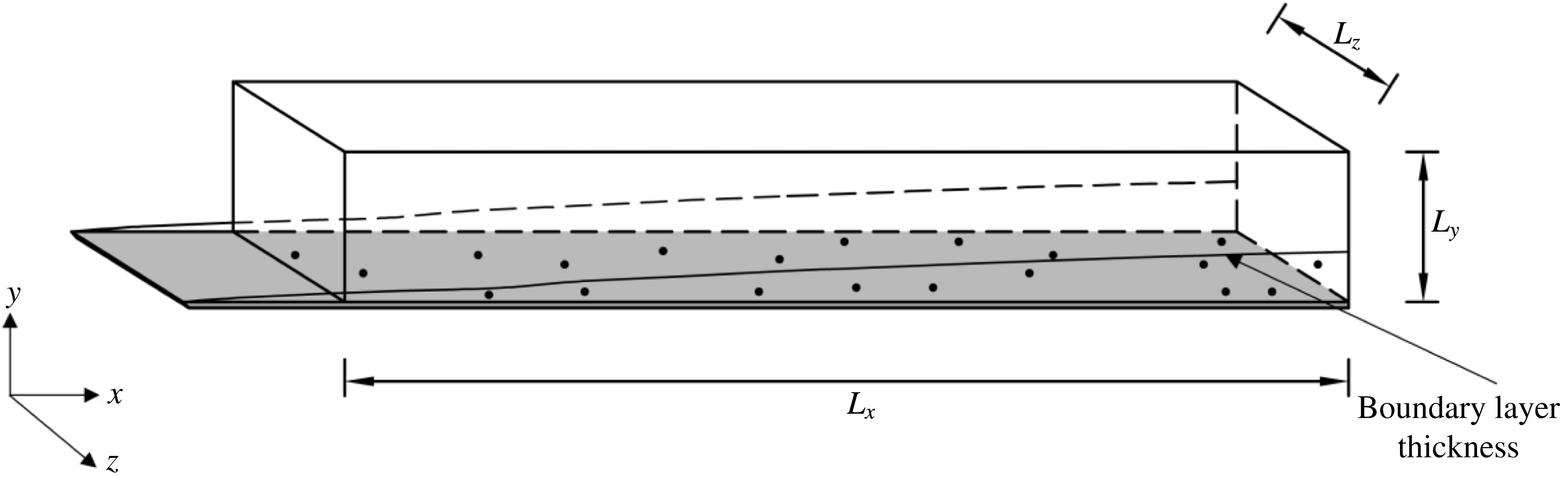
A graphical representation of the computational domain is given in figure 1. The origin of the Cartesian coordinate system is located at the leading edge of the flat plate (
 $x=0$
);
 $x$
,
 $y$
and
 $z$
are the coordinates in the streamwise, wall-normal and spanwise directions respectively. The domain size and mesh resolution are summarized in table 1. It should be noted that the variables written in wall units (identified by superscript
 $+$
) are non-dimensionalized using the wall-friction velocity
 $u_{\unicode[STIX]{x1D70F}}=0.0475$
in the turbulent region at
 $Re_{\unicode[STIX]{x1D703}}=900$
. The grid spacings are constant in the streamwise and spanwise directions, whereas in the wall-normal direction, the grid is stretched to resolve the near-wall boundary layer flow, with the closest grid point to the wall being located at
 $\unicode[STIX]{x0394}y_{min}^{+}=0.69$
.
The initial velocity field of the fluid is identical to a fully developed instantaneous velocity field computed by DNS of a single-phase spatially developing flat-plate boundary layer with the same mesh (table 1). The inflow boundary condition is similar to that of Wu & Moin (Reference Wu and Moin2009). In order to trigger breakdown of the laminar boundary layer to turbulence, the velocity field of the isotropic turbulence box is introduced into the computational domain every
 $3000\unicode[STIX]{x0394}t$
, where
 $\unicode[STIX]{x0394}t$
is the computational time step. It should be noted that the isotropic turbulent velocity field has been obtained from a precursor DNS of decaying homogeneous isotropic turbulence. At the inlet station, the isotropic turbulence box, with size
 $375\unicode[STIX]{x1D703}_{0}$
in each direction, is placed
 $15\unicode[STIX]{x1D703}_{0}$
away from the wall so that the laminar Blasius boundary layer will not be distorted by the imposed turbulent perturbations. That is, at the inlet,
 $Re_{\unicode[STIX]{x1D703}_{0}}=80$
, the isotropic turbulent velocity fluctuations are superposed on the free-stream velocity. The free-stream turbulence intensity is 8.3 % at the inlet and becomes negligible in the fully developed turbulent regime. A convective boundary condition (Orlanski Reference Orlanski1976) is specified at the outflow boundary. Periodic boundary conditions are applied along the homogeneous spanwise direction. At the top surface of the computational domain, the boundary conditions are
 $u=U_{\infty }$
,
 $v=V_{Blasius}$
and
 $w=0$
, as in Jacobs & Durbin (Reference Jacobs and Durbin2001) and Ovchinnikov, Choudhari & Piomelli (Reference Ovchinnikov, Choudhari and Piomelli2008). No-slip conditions,
 $u=0,v=0,w=0$
, are imposed at the solid wall.
Schematic diagram of the computational domain.

Domain size and mesh resolution.
 $L_{x}$
,
 $L_{y}$
and
 $L_{z}$
are the size of the computational domain, and
 $N_{x}$
,
 $N_{y}$
and
 $N_{z}$
are the corresponding numbers of grid points along the streamwise, wall-normal and spanwise directions respectively;
 $\unicode[STIX]{x0394}x^{+}$
and
 $\unicode[STIX]{x0394}z^{+}$
are the grid resolutions in the streamwise and spanwise directions respectively;
 $\unicode[STIX]{x0394}y_{min}^{+}$
is the minimum grid spacing and
 $\unicode[STIX]{x1D702}_{min}$
is the minimum Kolmogorov length scale in the wall-normal direction.

The fractional step algorithm is employed to solve the three-dimensional incompressible Navier–Stokes and continuity equations (Perot Reference Perot1993). The nonlinear and wall-parallel diffusion terms are treated explicitly, whereas the diffusion terms in the wall-normal direction are treated implicitly. The Navier–Stokes equations are time advanced using a low-storage third-order Runge–Kutta scheme for terms treated explicitly and a second-order Crank–Nicolson scheme for terms treated implicitly. A fourth-order-accurate finite difference scheme is employed to discretize the convective terms of the momentum equation on staggered grids and a higher-order Lagrange polynomial interpolation is used to discretize the viscous terms (Desjardins et al. Reference Desjardins, Blanquart, Balarac and Pitsch2008).
2.2 Governing equations of particle motion
It is assumed that all particles are pointwise rigid spheres with identical diameter
 $d_{p}$
and density
 $\unicode[STIX]{x1D70C}_{p}$
. The flow considered is dilute gas–solid flow and the interactions between particles can be neglected. To focus on particle–fluid interactions, the effect of gravity is not considered. Since the particles are much heavier than the fluid (
 $\unicode[STIX]{x1D70C}_{p}/\unicode[STIX]{x1D70C}_{f}=1500$
), the drag force is the main force acting on each particle (Elghobashi & Truesdell Reference Elghobashi and Truesdell1992; Boivin et al.
Reference Boivin, Simonin and Squires1998). Other forces such as buoyancy, pressure-gradient, Basset and virtual-mass forces are orders of magnitude smaller than the drag force and can therefore be ignored. However, the slip-shear lift force is taken into account because of the strong shear flows in the vicinity of the wall. In addition, since the particles may acquire very high angular velocities when they collide with the solid wall, the slip-rotation lift force is also considered in this study.
Therefore, the forces considered that act on the particles include the drag force, the slip-shear lift force and the slip-rotation lift force. The governing equations of the particles are expressed as follows:
 $$\begin{eqnarray}\displaystyle & \displaystyle \frac{\text{d}\boldsymbol{x}_{p}}{\text{d}t}=\boldsymbol{u}_{p}, & \displaystyle\end{eqnarray}$$
 $$\begin{eqnarray}\displaystyle & \displaystyle m_{p}\frac{\text{d}\boldsymbol{u}_{p}}{\text{d}t}=\boldsymbol{F}_{D}+\boldsymbol{F}_{LS}+\boldsymbol{F}_{LR}, & \displaystyle\end{eqnarray}$$
 $$\begin{eqnarray}\displaystyle & \displaystyle I_{p}\frac{\text{d}\unicode[STIX]{x1D74E}_{p}}{\text{d}t}=\boldsymbol{T}, & \displaystyle\end{eqnarray}$$
 $\boldsymbol{x}_{p}$
,
 $\boldsymbol{u}_{p}$
,
 $\unicode[STIX]{x1D74E}_{p}$
are respectively the position vector, linear velocity vector and angular velocity vector of the particles;
 $m_{p}=\unicode[STIX]{x03C0}\unicode[STIX]{x1D70C}_{p}d_{p}^{3}/6$
is the mass of the particle and
 $I_{p}=m_{p}d_{p}^{2}/10$
is the moment of inertia;
 $\boldsymbol{F}_{D}$
,
 $\boldsymbol{F}_{LS}$
,
 $\boldsymbol{F}_{LR}$
and
 $\boldsymbol{T}$
represent the drag force, the slip-shear lift force, the slip-rotation lift force and the torque respectively. They are given as follows:
 $$\begin{eqnarray}\displaystyle & \displaystyle \boldsymbol{F}_{D}=\frac{\unicode[STIX]{x1D70C}_{f}}{2}\frac{\unicode[STIX]{x03C0}}{4}d_{p}^{2}C_{D}|\boldsymbol{u}_{f}-\boldsymbol{u}_{p}|(\boldsymbol{u}_{f}-\boldsymbol{u}_{p}), & \displaystyle\end{eqnarray}$$
 $$\begin{eqnarray}\displaystyle & \displaystyle \boldsymbol{F}_{LS}=\frac{\unicode[STIX]{x1D70C}_{f}}{2}\frac{\unicode[STIX]{x03C0}}{4}d_{p}^{3}C_{LS}\{(\boldsymbol{u}_{f}-\boldsymbol{u}_{p})\times \unicode[STIX]{x1D74E}_{f}\}, & \displaystyle\end{eqnarray}$$
 $$\begin{eqnarray}\displaystyle & \displaystyle \boldsymbol{F}_{LR}=\frac{\unicode[STIX]{x1D70C}_{f}}{2}\frac{\unicode[STIX]{x03C0}}{4}d_{p}^{2}C_{LR}|\boldsymbol{u}_{f}-\boldsymbol{u}_{p}|\frac{\unicode[STIX]{x1D734}\times (\boldsymbol{u}_{f}-\boldsymbol{u}_{p})}{|\unicode[STIX]{x1D734}|}, & \displaystyle\end{eqnarray}$$
 $$\begin{eqnarray}\displaystyle & \displaystyle \boldsymbol{T}=\frac{\unicode[STIX]{x1D70C}_{f}}{2}\left(\frac{d_{p}}{2}\right)^{5}C_{R}|\unicode[STIX]{x1D734}|\unicode[STIX]{x1D734}, & \displaystyle\end{eqnarray}$$
 $\boldsymbol{u}_{f}$
is the fluid velocity vector at the particle position,
 $\unicode[STIX]{x1D74E}_{f}=1/2\unicode[STIX]{x1D735}\times \boldsymbol{u}_{f}$
is the fluid angular velocity vector and
 $\unicode[STIX]{x1D734}=\unicode[STIX]{x1D74E}_{f}-\unicode[STIX]{x1D74E}_{p}$
represents the relative rotation between fluid and particles. Here,
 $C_{D}$
is the drag coefficient, expressed as
 $$\begin{eqnarray}C_{D}=\frac{24}{Re_{p}}f_{D},\end{eqnarray}$$
where the drag factor
 $f_{D}$
is obtained from the correlation (Schiller & Naumann Reference Schiller and Naumann1933)
 $$\begin{eqnarray}f_{D}=1+0.15Re_{p}^{0.687},\end{eqnarray}$$
where
 $Re_{p}=d_{p}|\boldsymbol{u}_{f}-\boldsymbol{u}_{p}|/\unicode[STIX]{x1D708}$
is the particle Reynolds number. It should be noted that the expression for the drag force is applicable to particles smaller than the Kolmogorov length scale (Maxey & Riley Reference Maxey and Riley1983). According to Mei (Reference Mei1992), the slip-shear lift coefficient
 $C_{LS}$
in (2.7) is expressed as
 $$\begin{eqnarray}C_{LS}=\frac{4.1126}{Re_{s}^{0.5}}f(Re_{p},Re_{s}),\end{eqnarray}$$
where
 $Re_{s}=d_{p}^{2}|\unicode[STIX]{x1D74E}_{f}|/\unicode[STIX]{x1D708}$
is the Reynolds number of the shear flow and
 $f(Re_{p},Re_{s})$
is the ratio of the extended lift force to the Saffman force, given by
 $$\begin{eqnarray}f(Re_{p},Re_{s})=\left\{\begin{array}{@{}ll@{}}\displaystyle (1-0.3314\unicode[STIX]{x1D6FD}^{1/2})\exp \left(-\frac{Re_{p}}{10}\right)+0.3314\unicode[STIX]{x1D6FD}^{1/2},\quad & Re_{p}\leqslant 40,\\ \displaystyle 0.0524(\unicode[STIX]{x1D6FD}Re_{p})^{1/2},\quad & Re_{p}>40.\end{array}\right.\end{eqnarray}$$
Here, the parameter
 $\unicode[STIX]{x1D6FD}$
is defined as
 $$\begin{eqnarray}\unicode[STIX]{x1D6FD}=\frac{d_{p}|\unicode[STIX]{x1D74E}_{f}|}{2|\boldsymbol{u}_{f}-\boldsymbol{u}_{p}|}=\frac{1}{2}\frac{Re_{s}}{Re_{p}}.\end{eqnarray}$$
The slip-rotation lift coefficient
 $C_{LR}$
in (2.8) is obtained according to Rubinow & Keller (Reference Rubinow and Keller1961) and Oesterle & Dinh (Reference Oesterle and Dinh1998) in the form
 $$\begin{eqnarray}C_{LR}=\left\{\begin{array}{@{}ll@{}}\displaystyle \frac{Re_{R}}{Re_{p}},\quad & Re_{p}\leqslant 1,\\ \displaystyle 0.45+\left(\frac{Re_{R}}{Re_{p}}-0.45\right)\exp (-0.05684Re_{R}^{0.4}Re_{p}^{0.3}),\quad & 1<Re_{p}<140,\end{array}\right.\end{eqnarray}$$
where
 $Re_{R}$
is the Reynolds number of particle rotation,
 $Re_{R}=d_{p}^{2}|\unicode[STIX]{x1D734}|/\unicode[STIX]{x1D708}$
. According to previous research results (Rubinow & Keller Reference Rubinow and Keller1961; Sawatzki Reference Sawatzki1970; Dennis, Singh & Ingham Reference Dennis, Singh and Ingham1980), the rotational coefficient
 $C_{R}$
in (2.9) is found to be
 $$\begin{eqnarray}C_{R}=\left\{\begin{array}{@{}ll@{}}\displaystyle \frac{64\unicode[STIX]{x03C0}}{Re_{R}},\quad & Re_{R}\leqslant 32,\\ \displaystyle \frac{12.9}{Re_{R}^{0.5}}+\frac{128.4}{Re_{R}},\quad & 32<Re_{R}<1000.\end{array}\right.\end{eqnarray}$$
After all forces acting on the particles have been computed, the dimensionless equation to govern the particle motion can be written as
 $$\begin{eqnarray}\displaystyle \frac{\text{d}\boldsymbol{u}_{p}}{\text{d}t} & = & \displaystyle \boldsymbol{f}_{p}=\frac{f_{D}}{St}(\boldsymbol{u}_{f}-\boldsymbol{u}_{p})+\frac{3}{4}\frac{\unicode[STIX]{x1D70C}_{f}}{\unicode[STIX]{x1D70C}_{p}}C_{LS}\{(\boldsymbol{u}_{f}-\boldsymbol{u}_{p})\times \unicode[STIX]{x1D74E}_{f}\}\nonumber\\ \displaystyle & & \displaystyle +\,\frac{3}{4}\frac{\unicode[STIX]{x1D70C}_{f}}{\unicode[STIX]{x1D70C}_{p}}\frac{Re_{p}}{Re_{R}}C_{LR}\{\unicode[STIX]{x1D734}\times (\boldsymbol{u}_{f}-\boldsymbol{u}_{p})\},\end{eqnarray}$$
where
 $\boldsymbol{f}_{p}$
is the total force acting on the particles. The particle Stokes number
 $St$
is defined as the ratio of the particle relaxation time
 $\unicode[STIX]{x1D70F}_{p}$
to a characteristic flow time scale
 $\unicode[STIX]{x1D70F}_{f}$
:
 $$\begin{eqnarray}St=\frac{\unicode[STIX]{x1D70F}_{p}}{\unicode[STIX]{x1D70F}_{f}}=\frac{\unicode[STIX]{x1D70C}_{p}d_{p}^{2}/18\unicode[STIX]{x1D707}}{\unicode[STIX]{x1D703}_{0}/U_{\infty }},\end{eqnarray}$$
where
 $\unicode[STIX]{x1D707}$
is the dynamic viscosity of the fluid.
Considering that the volume fraction of the particles
 $\unicode[STIX]{x1D6F7}_{v}$
 $(6.67\times 10^{-5}\sim 6.67\times 10^{-4})$
is large enough to modulate the fluid turbulence, two-way coupling is assumed to model the interactions between fluid and particles. The feedback force performed by the particles on fluid grid point
 $m$
is given by
 $$\begin{eqnarray}\boldsymbol{f}_{m}=-\mathop{\sum }_{n=1}^{N_{p}}\frac{\unicode[STIX]{x1D70C}_{p}V_{p}}{\unicode[STIX]{x1D70C}_{f}V_{m}}\boldsymbol{f}_{p}^{n}S(\boldsymbol{x}^{n},\boldsymbol{x}^{m}),\end{eqnarray}$$
where
 $N_{p}$
denotes the instantaneous number of particles in the control volume,
 $V_{p}$
is the volume of particle
 $n$
and
 $V_{m}$
is the control volume of fluid grid
 $m$
;
 $\boldsymbol{f}_{p}^{n}$
represents the total force acting on particle
 $n$
given by (2.17). In order to ensure the conservation of global kinetic energy for the particle–fluid system, the weight function
 $S(\boldsymbol{x}^{n},\boldsymbol{x}^{m})$
locally distributes the backreaction force
 $\boldsymbol{f}_{p}^{n}$
on the Eulerian grid
 $m$
via the fourth-order Lagrangian interpolation scheme, which is also employed to evaluate the fluid velocity at the location of the particle. That is, the interpolation scheme used to redistribute the particle reaction force on the grid nodes is the same as that used to calculate the fluid velocity at the particle position. This model has been used for the study of turbulence modulation by Sundaram & Collins (Reference Sundaram and Collins1999).
2.3 Lagrangian particle tracking
In this paper, the Eulerian–Lagrangian point-particle approach is employed to simulate the particle-laden turbulent flows. The particles are tracked individually through the integration of Lagrangian equation (2.3)–(2.5) with the same time step as the Eulerian fluid equation (2.1), (2.2). The particle linear and angular velocities are integrated by an explicit third-order Runge–Kutta scheme and the particle position by a second-order Crank–Nicolson scheme. At the beginning of the Lagrangian tracking, a large number of solid particles are released randomly inside the boundary layer zone
 $(y\leqslant 120\unicode[STIX]{x1D703}_{0})$
of the single-phase flow. It should be noted that at the outflow plane, the boundary layer thickness is
 $120\unicode[STIX]{x1D703}_{0}$
for the single-phase flow. The initial velocity of each particle is set equal to the local fluid velocity evaluated at the centre of the particle. The fourth-order Lagrange polynomials are used to calculate the fluid velocity at the position of the particle (near the wall, the interpolation scheme switches to one-sided). Periodic boundary conditions are imposed on particles moving outside the computational domain along the spanwise direction. In order to keep the particle number constant, when one particle exits the computational domain from the outlet plane, another particle is randomly injected into the domain from the inlet plane. The height of the domain is large enough so that particles cannot pass through the upper boundary. Perfectly elastic particle–wall collisions are assumed when a particle reaches a distance lower than one particle radius from the wall. A detailed description of the principles and algorithm used to compute particle–wall collisions can be found in Yamamoto et al. (Reference Yamamoto, Potthoff, Tanaka, Kajishima and Tsuji2001).
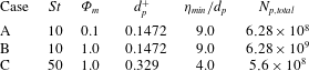
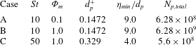
In order to reveal the turbulence modulation, three cases with different particle mass loadings and different particle Stokes numbers are simulated and compared. Table 2 shows the various parameters of the tracked particles in the three cases, including the Stokes number
 $St$
, the particle mass loading
 $\unicode[STIX]{x1D6F7}_{m}$
, the particle diameter
 $d_{p}^{+}$
, the ratio of the minimum Kolmogorov length scale
 $\unicode[STIX]{x1D702}_{min}$
to the particle diameter
 $d_{p}$
and the total number of particles tracked
 $N_{p,total}$
. The maximum diameter of the particles with
 $St=50$
is much smaller than the Kolmogorov length scale, and thus the requirements imposed by the point-particle approach can be satisfied.
Parameters of the tracked particles for the three simulations studied.
The simulations were run on 1024 cores using message-passing-interface (MPI) parallelization. The Eulerian–Lagrangian point-particle code has been validated for the simulation of boundary layer flows in our recent study (Li et al.
Reference Li, Wei, Luo and Fan2016). The non-dimensional time step in wall units was set to be
 $\unicode[STIX]{x0394}t^{+}=0.09$
, which was confirmed by the simulated results to be small enough that a particle could not pass through more than half a grid cell per iterative step. The flow field and particle concentration reached statistically quasi-steady state after
 $70\,000\unicode[STIX]{x0394}t$
. Statistics were then collected for another
 $60\,000\unicode[STIX]{x0394}t$
. It should be noted that the statistical results have been computed by averaging over time as well as over the homogeneous spanwise direction.
Instantaneous snapshots of the three-dimensional flow field and the particle configuration inside the computational domain for case A, using contours of instantaneous streamwise velocity. It should be noted that the particles are indicated here by small golden spheres.

3 Turbulence modulation by particles
This section provides an overview of the effect of inertial particles on the skin-friction and boundary layer integral parameters and some important turbulence statistics. Selected results obtained from the DNS are presented, with the focus on comparisons between single-phase and particle-laden flows. It should be pointed out that in this paper, all variables written in either inner wall units or outer units are non-dimensionalized using the parameters (e.g. friction velocity) of the single-phase boundary layer flow.
Figure 2 shows instantaneous snapshots of the three-dimensional flow field and the particle distribution for case A, using the contours of the instantaneous streamwise velocity. It should be noted that only a quarter of the wall-normal lengths are presented in this figure for better visibility, and that the inertial solid particles are indicated by small golden spheres. The contours of the streamwise velocity at the bottom plane located in the viscous sublayer with
 $y^{+}=5$
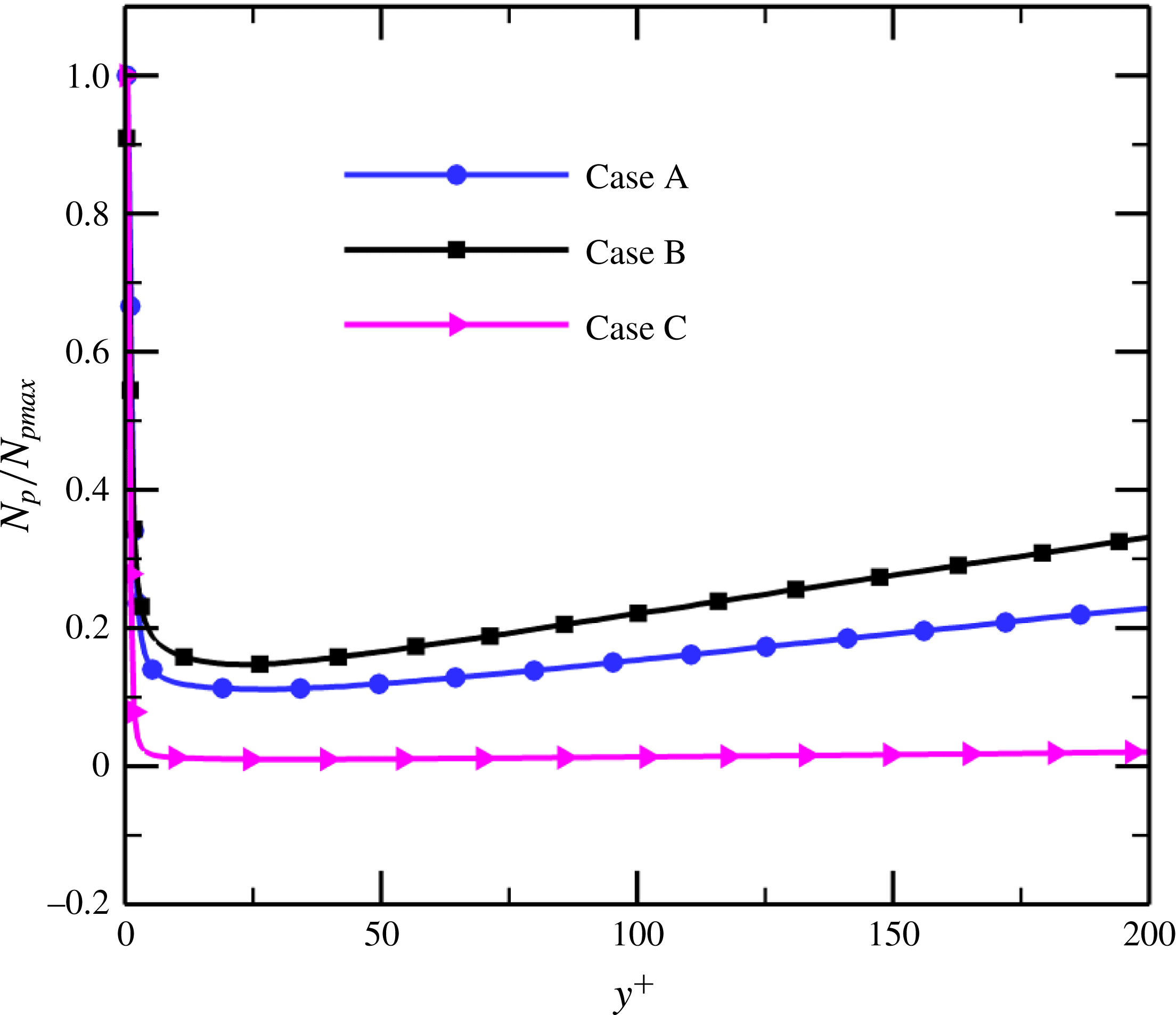
clearly highlight the near-wall high- and low-speed streaks. Although the particles are introduced randomly into the computational domain at the beginning of the simulations, the inertial particles tend to move towards the wall, as shown by the particle number density profile in figure 3 for the three different cases. The particle number density
 $N_{p}$
is normalized by its maximum value
 $N_{pmax}$
. In our previous study (Li et al.
Reference Li, Wei, Luo and Fan2016), we investigated the mechanism of particle preferential distribution in a flat-plate boundary layer and found that near-wall quasi-streamwise vortices were responsible.
Wall-normal profiles of the particle number density in the particle-laden flows at
 $x=4867\unicode[STIX]{x1D703}_{0}$
.

3.1 Skin-friction and integral parameters
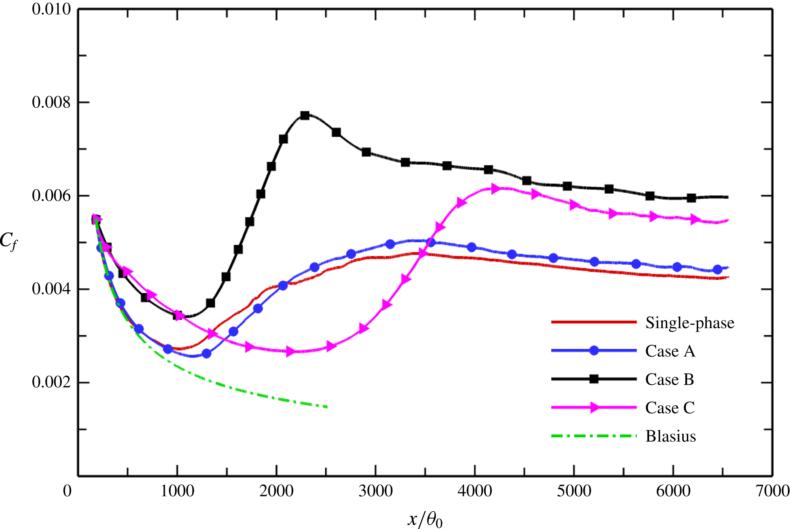
The evolution of the mean skin-friction coefficient
 $$\begin{eqnarray}C_{f}=\frac{\unicode[STIX]{x1D707}\unicode[STIX]{x2202}\bar{u}/\unicode[STIX]{x2202}y|_{y=0}}{1/2\,\unicode[STIX]{x1D70C}U_{\infty }^{2}}\end{eqnarray}$$
along the flat plate is reported in figure 4. For a quantitative comparison, the single-phase data (Li et al.
Reference Li, Wei, Luo and Fan2016) and the Blasius solution are also plotted on the same axes. It is well known that
 $C_{f}$
is an excellent indicator of the laminar, transitional and turbulent regions in boundary layer flow. The locations of the onset and completion of transition are identified by the local minimum and maximum of
 $C_{f}$
respectively (Jacobs & Durbin Reference Jacobs and Durbin2001; Sayadi, Hamman & Moin Reference Sayadi, Hamman and Moin2013). In the laminar region, the inertial particles with lower mass loading
 $\unicode[STIX]{x1D6F7}_{m}=0.1$
(case A) have an insignificant effect on the mean skin-friction coefficient
 $C_{f}$
, which follows the Blasius profile, like single-phase flow. As the particle mass loading increases, however, the particles with
 $\unicode[STIX]{x1D6F7}_{m}=1.0$
(cases B and C) substantially alter the laminar flow state, and
 $C_{f}$
deviates from the Blasius solution nearly from the inflow plane. In addition, the presence of particles has a remarkable influence on the transition process of the boundary layer. Compared with the single-phase case, the particles with smaller Stokes number
 $St=10$
cause a slight delay in the onset of transition, while the larger particles with
 $St=50$
cause a significant delay. The completion of transition for case B with higher mass loading
 $\unicode[STIX]{x1D6F7}_{m}=1.0$
is earlier than those for both the unladen case and case A with lower mass loading.
Evolution of the mean skin-friction coefficient
 $C_{f}$
with
 $x/\unicode[STIX]{x1D703}_{0}$
along the flat plate.

It is evident that the solid particles significantly increase the mean skin-friction coefficient
 $C_{f}$
, especially in the turbulent region. Furthermore, the degree of enhancement increases with particle mass loading. However, the smaller particles with
 $St=10$
(case B) appear to have a more pronounced effect on the skin-friction coefficient than the larger ones with
 $St=50$
(case C) for the same mass loading. As will be shown later, the increase of the skin-friction drag in the particle-laden flows can be explained in terms of an increased velocity gradient near the wall.
The characteristics of the boundary layer change as the flow moves downstream, since the flow over a flat plate develops spatially in the streamwise direction. Figure 5 shows the variations of the boundary layer integral parameters, namely the boundary layer thickness
 $\unicode[STIX]{x1D6FF}$
, the displacement thickness
 $\unicode[STIX]{x1D6FF}^{\ast }$
, the momentum thickness
 $\unicode[STIX]{x1D703}$
and the kinetic energy thickness
 $\unicode[STIX]{x1D6FF}^{\ast \ast }$
, along the plate, i.e. with the streamwise coordinate
 $x/\unicode[STIX]{x1D703}_{0}$
. These integral parameters are defined as follows:
 $$\begin{eqnarray}\displaystyle & \displaystyle \unicode[STIX]{x1D6FF}=0.99U_{\infty }, & \displaystyle\end{eqnarray}$$
 $$\begin{eqnarray}\displaystyle & \displaystyle \unicode[STIX]{x1D6FF}^{\ast }=\int _{0}^{\unicode[STIX]{x1D6FF}}(1-\bar{u})\,\text{d}y, & \displaystyle\end{eqnarray}$$
 $$\begin{eqnarray}\displaystyle & \displaystyle \unicode[STIX]{x1D703}=\int _{0}^{\unicode[STIX]{x1D6FF}}\bar{u}(1-\bar{u})\,\text{d}y, & \displaystyle\end{eqnarray}$$
 $$\begin{eqnarray}\displaystyle & \displaystyle \unicode[STIX]{x1D6FF}^{\ast \ast }=\int _{0}^{\unicode[STIX]{x1D6FF}}\bar{u}(1-\bar{u}^{2})\,\text{d}y, & \displaystyle\end{eqnarray}$$
 $\bar{u}$
is the mean streamwise velocity. It can be observed that in the particle-laden flows, the displacement thickness, momentum thickness and kinetic energy thickness are all reduced at almost all streamwise locations, with the degree of reduction increasing with particle Stokes number and mass loading. In the turbulent region, the boundary layer thickness
 $\unicode[STIX]{x1D6FF}$
is also reduced in the particle-laden flow compared with the single-phase flow. However, it is interesting to note that the laminar boundary layer thickness is not significantly affected by the particles, even at higher mass loading
 $\unicode[STIX]{x1D6F7}_{m}=1.0$
(case B) or larger Stokes number
 $St=50$
(case C). This is in contrast to the other integral parameters, which are significantly affected by the particles with higher mass loading
 $\unicode[STIX]{x1D6F7}_{m}=1.0$
in the laminar region. It seems that the boundary layer thickness
 $\unicode[STIX]{x1D6FF}$
, whose definition is based simply on 99 % of the constant free-stream velocity and which has no further physical interpretation, is not a sensitive measure of the effect of the particles on the fluid.
Variation of the boundary layer integral parameters with the streamwise coordinate
 $x/\unicode[STIX]{x1D703}_{0}$
along the plate: (a) boundary layer thickness
 $\unicode[STIX]{x1D6FF}$
; (b) displacement thickness
 $\unicode[STIX]{x1D6FF}^{\ast }$
; (c) momentum thickness
 $\unicode[STIX]{x1D703}$
; (d) kinetic energy thickness
 $\unicode[STIX]{x1D6FF}^{\ast \ast }$
.

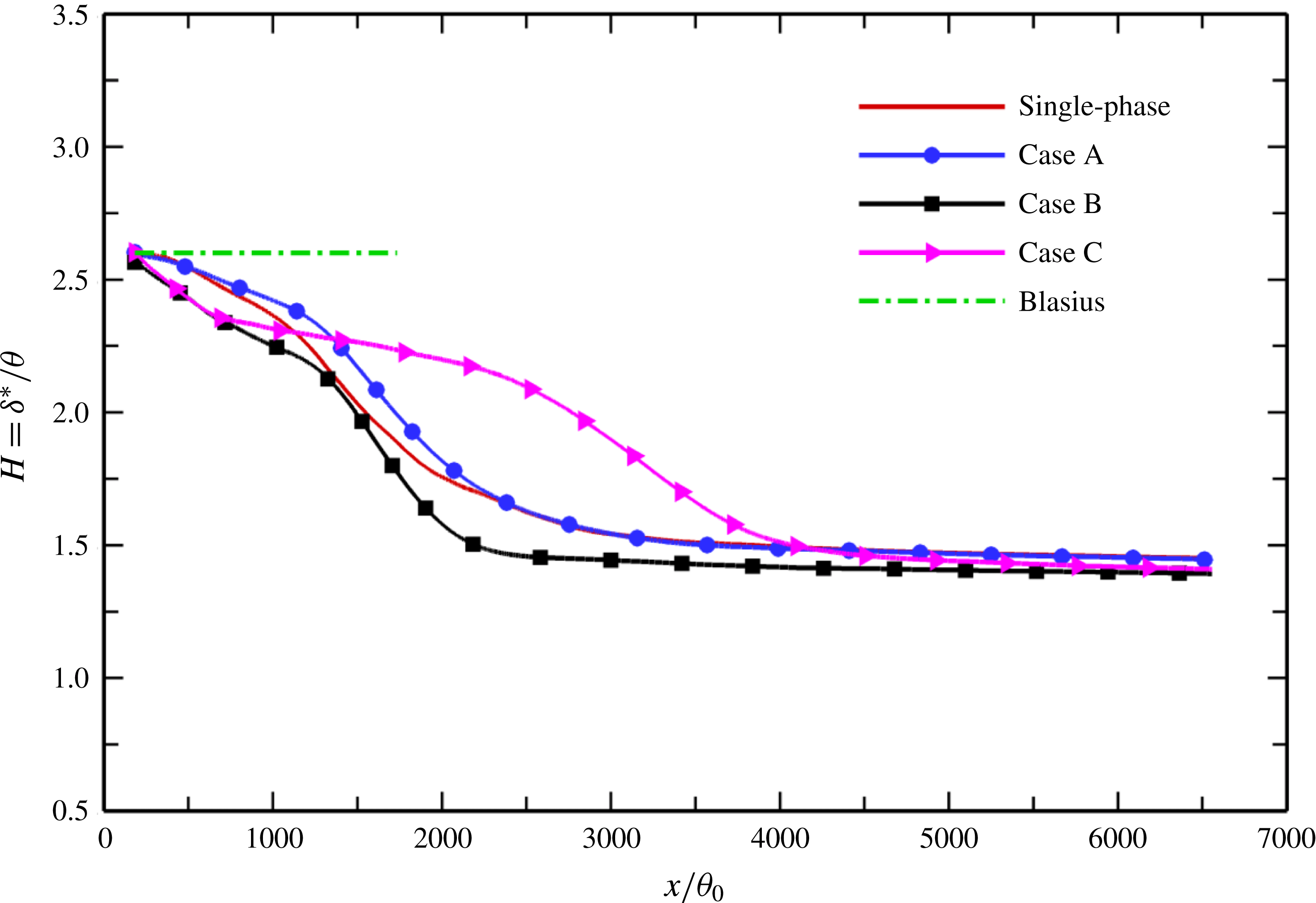
The streamwise development of the shape factor
 $H=\unicode[STIX]{x1D6FF}^{\ast }/\unicode[STIX]{x1D703}$
is presented in figure 6. The effect of particles on the shape factor clearly depends on the particle mass loading and Stokes number. For case A with lower mass loading
 $\unicode[STIX]{x1D6F7}_{m}=0.1$
, the shape factor increases slightly in the transitional region but remains almost unchanged in the turbulent region. Although both the displacement thickness and the momentum thickness are reduced in the particle-laden flows, the particles in case B with higher mass loading
 $\unicode[STIX]{x1D6F7}_{m}=1.0$
have a stronger effect on the displacement thickness, which results in an overall reduction of the shape factor in the streamwise direction. This means that for case B, the displacement thickness decreases at a higher rate compared with the momentum thickness. The particles with larger inertia
 $St=50$
, on the other hand, exhibit an opposite effect on the shape factor; that is, the momentum thickness decreases more rapidly than the displacement thickness in case C. It is noteworthy that all of the shape factors in the three different particle-laden simulations are almost identical to that of the single-phase case in the fully developed turbulent region, implying that the presence of particles has an almost negligible effect on the shape factor when the flow becomes turbulent.
Variation of the shape factor
 $H$
with
 $x/\unicode[STIX]{x1D703}_{0}$
along the plate.

3.2 Mean velocity statistics
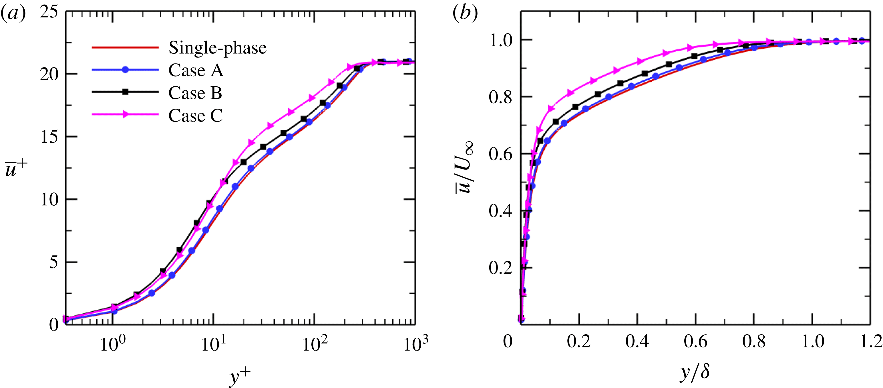
Figure 7 shows the mean streamwise velocity profiles plotted versus the inner wall coordinate
 $y^{+}$
and the outer wall-normal coordinate
 $y/\unicode[STIX]{x1D6FF}$
at the same streamwise location
 $x=4867\unicode[STIX]{x1D703}_{0}$
. It should be noted that the location
 $x=4867\unicode[STIX]{x1D703}_{0}$
in the particle-laden flows corresponds to the turbulent station
 $Re_{\unicode[STIX]{x1D703}}=900$
in single-phase flow. It can be seen that the solid particles substantially increase the mean streamwise velocity in the particle-laden flows, which is consistent with previous results in wall-bounded turbulent flows such as channel and pipe flows (Pan & Banerjee Reference Pan and Banerjee1996; Li et al.
Reference Li, McLaughlin, Kontomaris and Portela2001; Zhao et al.
Reference Zhao, Andersson and Gillissen2013). The higher the particle mass loading is, the more intense this effect is. Comparing case B with case C, it is found that in the logarithmic layer, the larger particles with
 $St=50$
have a stronger effect on the mean velocity than the smaller particles with
 $St=10$
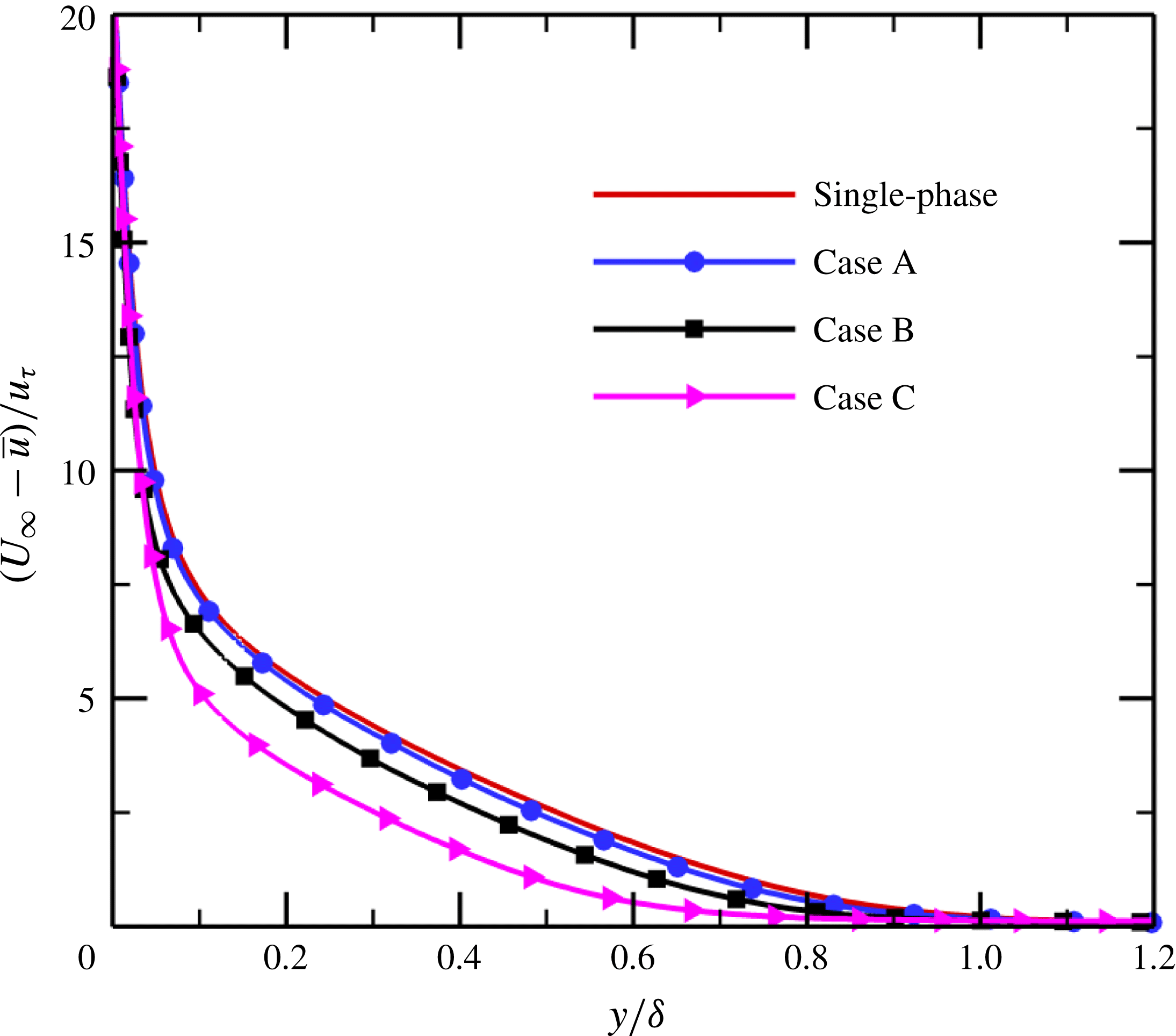
, while the opposite is true in the viscous sublayer. It should be pointed out that the reductions in the boundary layer integral parameters (figure 5), as discussed previously, can be explained by the enhancement of the mean streamwise velocity. The mean velocity deficit
 $(U_{\infty }-\bar{u})/u_{\unicode[STIX]{x1D70F}}$
is displayed in figure 8 using the outer coordinate
 $y/\unicode[STIX]{x1D6FF}$
. It is clear that the presence of particles causes a progressive decrease in the velocity defect profile with increasing particle mass loading
 $\unicode[STIX]{x1D6F7}_{m}$
and Stokes number
 $St$
, as a consequence of the increased mean streamwise velocity.
Figure 9 reports the profiles of the mean velocity gradients
 $\text{d}\bar{u}^{+}/\text{d}\ln y^{+}$
and
 $\text{d}\ln \bar{u}^{+}/\text{d}\ln y^{+}$
versus the inner wall coordinate
 $y^{+}$
at streamwise coordinate
 $x=4867\unicode[STIX]{x1D703}_{0}$
. The addition of inertial particles significantly increases the local velocity gradient
 $\text{d}\bar{u}/\text{d}y$
in the near-wall regions, with the effect being greater at higher mass loading; see figure 9(a). The enhancement of the streamwise velocity gradient close to the wall in the particle-laden flows leads to an obvious increase in skin-friction drag, as shown in figure 4. It is noticeable that the particles with smaller inertia displace the profile of the velocity gradient towards the wall, and the level of displacement increases with particle mass loading. The larger particles in case C with
 $St=50$
produce a remarkable increase in the velocity gradient in the buffer layer but noticeable decreases in the logarithmic layer and the outer layer.
Mean streamwise velocity profiles in the turbulent region at
 $x=4867\unicode[STIX]{x1D703}_{0}$
: (a) versus the inner wall coordinate
 $y^{+}$
; (b) versus the outer wall-normal coordinate
 $y/\unicode[STIX]{x1D6FF}$
.

Mean velocity defect profile
 $(U_{\infty }-\bar{u})/u_{\unicode[STIX]{x1D70F}}$
versus the outer coordinate
 $y/\unicode[STIX]{x1D6FF}$
at
 $x=4867\unicode[STIX]{x1D703}_{0}$
.

Mean velocity gradients versus the inner wall coordinate
 $y^{+}$
at
 $x=4867\unicode[STIX]{x1D703}_{0}$
: (a)
 $\text{d}\bar{u}^{+}/\text{d}\ln y^{+}$
; (b)
 $\text{d}\ln \bar{u}^{+}/\text{d}\ln y^{+}$
.

As is well known, the logarithmic layer is a region in which the velocity gradient
 $\text{d}\bar{u}^{+}/\text{d}\ln y^{+}$
remains constant and equal to
 $1/\unicode[STIX]{x1D705}$
owing to the fact that the profile of the mean streamwise velocity follows the logarithmic law
 $\bar{u}^{+}=\ln y^{+}/\unicode[STIX]{x1D705}+C$
in this region, where
 $\unicode[STIX]{x1D705}$
is the von Kármán constant and
 $C$
is an additive constant. It can be observed that the logarithmic region is progressively shifted towards the wall as the particle mass loading increases. Furthermore, the logarithmic layer becomes shorter and narrower with increasing mass loading. It can also be observed that for the cases with larger mass loading (cases B and C), the velocity gradient
 $\text{d}\bar{u}^{+}/\text{d}\ln y^{+}$
is reduced in the logarithmic layer, i.e. the von Kármán constant
 $\unicode[STIX]{x1D705}$
is increased, resulting in a smaller slope of the logarithmic layer (figure 7
a). The increased value of
 $\unicode[STIX]{x1D705}$
usually suggests an increase in the skin-friction drag (Virk Reference Virk1975), which is consistent with the present simulation results.
As mentioned above, the particles cause an increase in the mean streamwise velocity
 $\bar{u}^{+}$
(figure 7
a) and the near-wall velocity gradient
 $\text{d}\bar{u}^{+}/\text{d}\ln y^{+}$
(figure 9
a). The fact that
 $\text{d}\ln \bar{u}^{+}/\text{d}\ln y^{+}$
is reduced with increasing particle mass loading, as shown in figure 9(b), indicates that the particles have a greater effect on the mean streamwise velocity
 $\bar{u}$
than on the mean velocity gradient
 $\text{d}\bar{u}/\text{d}y$
.
3.3 Second-order statistics
Figure 10 shows comparisons of turbulence intensities and Reynolds stress between single-phase and particle-laden flows in the turbulent region at
 $x=4867\unicode[STIX]{x1D703}_{0}$
. In the very-near-wall region, the streamwise turbulence intensity is slightly augmented in the cases with higher mass loading
 $\unicode[STIX]{x1D6F7}_{m}=1.0$
. Nevertheless, the presence of particles leads to a remarkable suppression of streamwise velocity fluctuation in the outer layer, and the level of suppression increases with particle mass loading. From a comparison of case B with case C, it appears that the turbulence damping is greater for smaller particles in the streamwise direction. The turbulence intensities in the wall-normal and spanwise directions are substantially attenuated across the entire boundary layer, as is the Reynolds stress. As the particle mass loading and Stokes number increase, the degree of attenuation increases. The enhancement or suppression of turbulence due to the presence of particles can be explained in terms of kinetic energy transfer between the particles and the fluid (see § 5).
Comparisons of turbulence intensities and Reynolds stress between single-phase and particle-laden flows in the turbulent region at
 $x=4867\unicode[STIX]{x1D703}_{0}$
: (a) streamwise turbulence intensity
 $u_{rms}^{^{\prime }+}$
; (b) wall-normal turbulence intensity
 $v_{rms}^{^{\prime }+}$
; (c) spanwise turbulence intensity
 $w_{rms}^{^{\prime }+}$
; (d) Reynolds stress
 $-\overline{u^{\prime }v^{^{\prime }}}^{\,+}$
.

As mentioned in § 1, a large number of experiments and numerical simulations have been performed to study turbulence modulation in particle-laden pipe or channel flows during the past few decades. Here, it is meaningful to carry out a comparison of turbulence modulation between turbulent pipe or channel flows and the turbulent boundary layer flow over a flat plate. In most cases, particles smaller than the Kolmogorov length scale tend to attenuate the Reynolds stress and the velocity fluctuations in the directions perpendicular to the mean flow, and the levels of attenuation increase monotonically with the particle mass loading
 $\unicode[STIX]{x1D6F7}_{m}$
. However, the streamwise turbulence intensity can be enhanced (Zhao et al.
Reference Zhao, Andersson and Gillissen2010, Reference Zhao, Andersson and Gillissen2013) or suppressed (Kulick et al.
Reference Kulick, Fessler and Eaton1994; Pan & Banerjee Reference Pan and Banerjee1996; Nasr, Ahmadi & McLaughlin Reference Nasr, Ahmadi and McLaughlin2009). In addition, Li et al. (Reference Li, McLaughlin, Kontomaris and Portela2001) and Dritselis & Vlachos (Reference Dritselis and Vlachos2008, Reference Dritselis and Vlachos2011) observed in a vertical channel flow that the presence of inertial particles attenuated the streamwise fluctuating velocity near the wall but augmented it in the outer flow region, which is exactly opposite to our numerical results for turbulent boundary layer flow. Another difference among wall-bounded turbulent flows is the effect of particle Stokes number on turbulence modulation. For cases with smaller particles,
 $d_{p}<\unicode[STIX]{x1D702}$
, some researchers reported that turbulence attenuation increased monotonically with increasing particle Stokes number
 $St$
(Kulick et al.
Reference Kulick, Fessler and Eaton1994; Zhao et al.
Reference Zhao, Andersson and Gillissen2013). However, the reverse has been found in some studies; that is, particles with larger inertia have a smaller effect on turbulent velocity fluctuations (Li et al.
Reference Li, McLaughlin, Kontomaris and Portela2001; Dritselis & Vlachos Reference Dritselis and Vlachos2011).
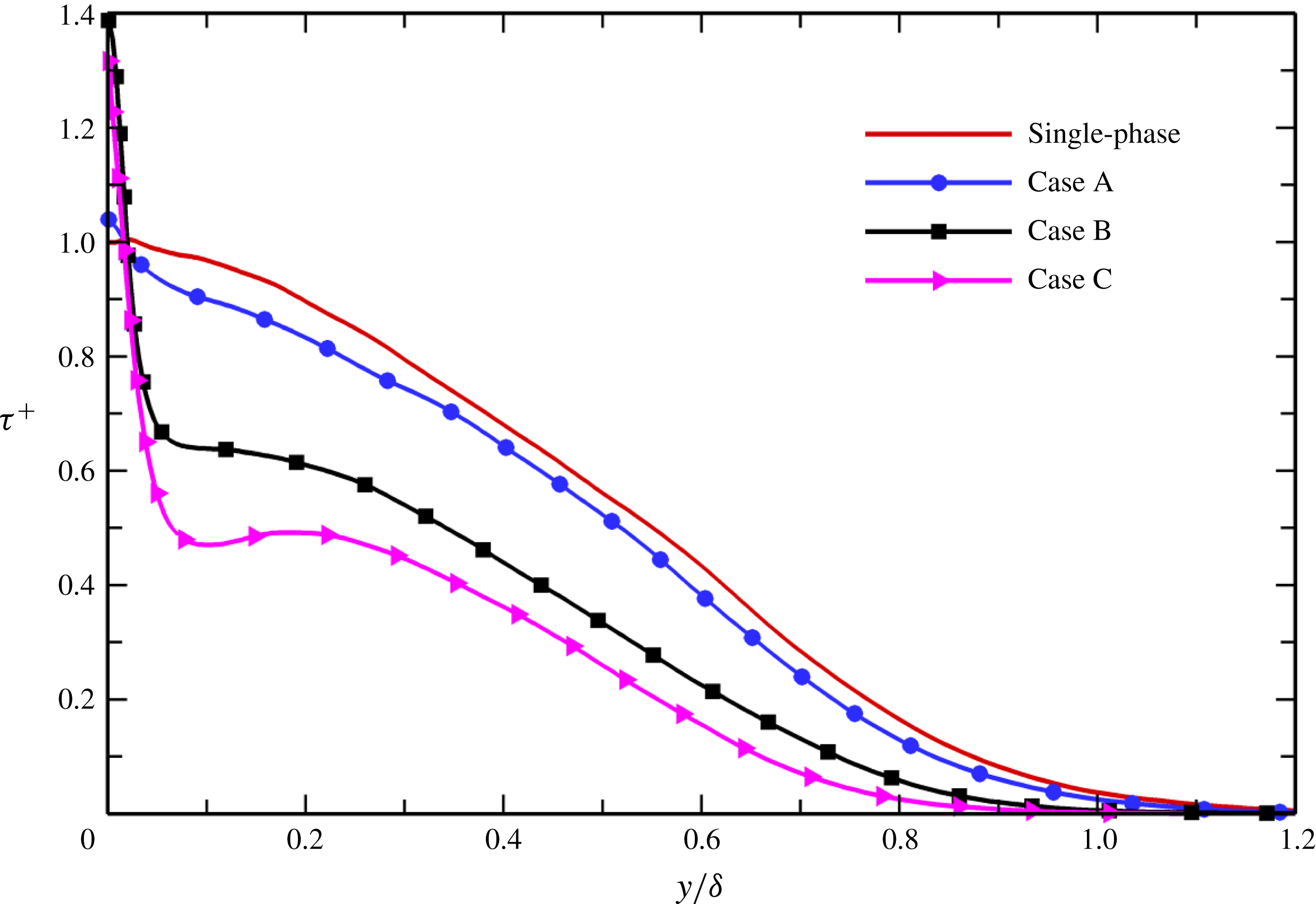
Total shear stress versus the outer wall coordinate
 $y/\unicode[STIX]{x1D6FF}$
at
 $x=4867\unicode[STIX]{x1D703}_{0}$
.

The total shear stress
 $\unicode[STIX]{x1D70F}^{+}=-\overline{u^{\prime }v^{^{\prime }}}^{\,+}+(\unicode[STIX]{x1D708}\text{d}\bar{u}/\text{d}y)^{+}$
in the turbulent region at
 $x=4867\unicode[STIX]{x1D703}_{0}$
is plotted in figure 11 using the outer wall coordinate
 $y/\unicode[STIX]{x1D6FF}$
. It is notable that in the single-phase flow, the total shear stress exhibits an overshoot in the very-near-wall region. Wu & Moin (Reference Wu and Moin2009) also observed this behaviour and ascribed it to a residual effect of boundary layer transition, and it will gradually disappear as the boundary layer develops downstream. However, the overshoot is absent in the particle-laden flows. The maximum total shear stress is obtained at the wall and
 $\unicode[STIX]{x1D70F}^{+}$
decreases monotonically along the wall-normal direction. In the present particle-laden flows, the Reynolds stress
 $-\overline{u^{\prime }v^{^{\prime }}}^{\,+}$
is reduced (figure 10
d), whereas the near-wall mean streamwise velocity gradient
 $\text{d}\bar{u}/\text{d}y$
is increased (figure 9
a). The combination of these two counteracting effects leads to an increase in the total shear stress in the close vicinity of the wall, owing to the fact that the rate of increase of the velocity gradient close to the wall is larger than the rate of decrease of the Reynolds stress. The enhancement of the total shear stress is more pronounced as the particle mass loading increases. It is noteworthy that for cases with higher mass loading
 $\unicode[STIX]{x1D6F7}_{m}=1.0$
, after a rapid decrease in the near-wall region, there exists a constant-stress layer in which the variations of
 $-\overline{u^{\prime }v^{^{\prime }}}^{\,+}$
and
 $(\unicode[STIX]{x1D708}\,\text{d}\bar{u}/\text{d}y)^{+}$
tend to cancel each other. However, this peculiar feature is not present either in single-phase flow or in case A with lower loading. Far from the wall, the total shear stress decreases monotonically with increasing mass loading
 $\unicode[STIX]{x1D6F7}_{m}$
and Stokes number
 $St$
, since both
 $-\overline{u^{\prime }v^{^{\prime }}}^{\,+}$
and
 $(\unicode[STIX]{x1D708}\,\text{d}\bar{u}/\text{d}y)^{+}$
are reduced in the outer wall layer and the degrees of reduction increase at higher
 $\unicode[STIX]{x1D6F7}_{m}$
and
 $St$
. As a result, the particles will produce strong damping of the production of turbulent kinetic energy,
 $P=-\overline{u^{\prime }v^{^{\prime }}}^{\,+}\text{d}\bar{u}^{+}/\text{d}y^{+}$
, as will be discussed below.
Figure 12 reports the turbulent kinetic energy
 $K=(\overline{u^{\prime }u^{\prime }}^{\,+}+\overline{v^{\prime }v^{\prime }}^{\,+}+\overline{w^{\prime }w^{\prime }}^{\,+})/2$
versus the inner wall coordinate
 $y^{+}$
at
 $x=4867\unicode[STIX]{x1D703}_{0}$
. The presence of inertial particles markedly damps the turbulent kinetic energy in the particle-laden flows, with the effect becoming more intense as the particle mass loading increases. The damping of turbulence production by particles, as shown below, can explain the reduced turbulent kinetic energy. In this context, we try to investigate the mechanism from an energetic point of view.
Turbulent kinetic energy
 $K=(\overline{u^{\prime }u^{\prime }}^{\,+}+\overline{v^{\prime }v^{\prime }}^{\,+}+\overline{w^{\prime }w^{\prime }}^{\,+})/2$
in the turbulent region at
 $x=4867\unicode[STIX]{x1D703}_{0}$
.

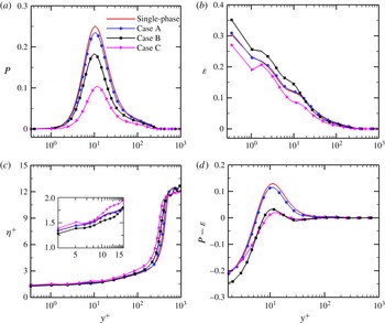
The rate of production of turbulent kinetic energy,
 $P=-\overline{u^{\prime }v^{\prime }}^{\,+}\text{d}\bar{u}^{+}/\text{d}y^{+}$
, is shown in figure 13(a). As expected, the energy production term
 $P$
is significantly decreased under the effect of particles. Furthermore, the degree of reduction increases with the particle Stokes number and mass loading. In particular, the peak value of
 $P$
in case C decreases by almost half compared with the unladen flow. Figure 13(b) shows the viscous dissipation rate of the turbulent kinetic energy,
 $\unicode[STIX]{x1D700}=\unicode[STIX]{x1D708}\overline{(\unicode[STIX]{x2202}u_{i}^{\prime }/\unicode[STIX]{x2202}x_{j})(\unicode[STIX]{x2202}u_{i}^{\prime }/\unicode[STIX]{x2202}x_{j})}$
, normalized by
 $u_{\unicode[STIX]{x1D70F}}^{4}/\unicode[STIX]{x1D708}$
(index notation is used here). For smaller particles with
 $St=10$
, the viscous dissipation rate is obviously enhanced near the wall, while it is decreased in the outer layer, as the particle mass loading increases. However, larger particles with
 $St=50$
seem to suppress viscous energy dissipation. The increase in viscous dissipation rate for smaller particles near the wall leads to a decrease in the Kolmogorov length scale because
 $\unicode[STIX]{x1D702}=(\unicode[STIX]{x1D708}^{3}/\unicode[STIX]{x1D700})^{1/4}$
, and the reverse is true in the region far away from the wall; see figure 13(c). Moreover, the enhancement of the Kolmogorov length scale increases monotonically with increasing particle Stokes number and mass loading in the outer layer.
Wall-normal distributions at
 $x=4867\unicode[STIX]{x1D703}_{0}$
of (a) the production rate of turbulent kinetic energy,
 $P=-\overline{u^{\prime }v^{^{\prime }}}^{\,+}\text{d}\bar{u}^{+}/\text{d}y^{+}$
, (b) the viscous dissipation rate
 $\unicode[STIX]{x1D700}$
, (c) the Kolmogorov length scale
 $\unicode[STIX]{x1D702}^{+}$
and (d) the difference between the production rate and the viscous dissipation rate,
 $P-\unicode[STIX]{x1D700}$
. It should be noted that the energy production term
 $P$
and the viscous dissipation term
 $\unicode[STIX]{x1D700}$
are normalized by
 $u_{\unicode[STIX]{x1D70F}}^{4}/\unicode[STIX]{x1D708}$
.
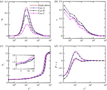
Figure 13(d) shows a comparison between the production rate of turbulent kinetic energy
 $P$
and the viscous dissipation rate
 $\unicode[STIX]{x1D700}$
. The production rate
 $P$
is lower than the viscous dissipation rate
 $\unicode[STIX]{x1D700}$
in the viscous sublayer, but
 $P>\unicode[STIX]{x1D700}$
in the buffer and logarithmic layers. In the outer region of the boundary layer, however, the rate of production of turbulent kinetic energy is approximately balanced by the rate of viscous dissipation, i.e.
 $P\approx \unicode[STIX]{x1D700}$
. In spite of the suppression of viscous energy dissipation in some cases, as noted above, the difference between the production rate and the viscous dissipation rate is decreased in the particle-laden flows compared with the unladen flow, and the effect is more pronounced at higher mass loading. Therefore, we can conclude that the presence of small solid particles damps the turbulent kinetic energy. It should be pointed out that particle–fluid interactions will produce extra energy dissipation, in addition to the viscous dissipation, which is a result of the turbulent energy cascade from larger to smaller eddies, as will be discussed in § 5.
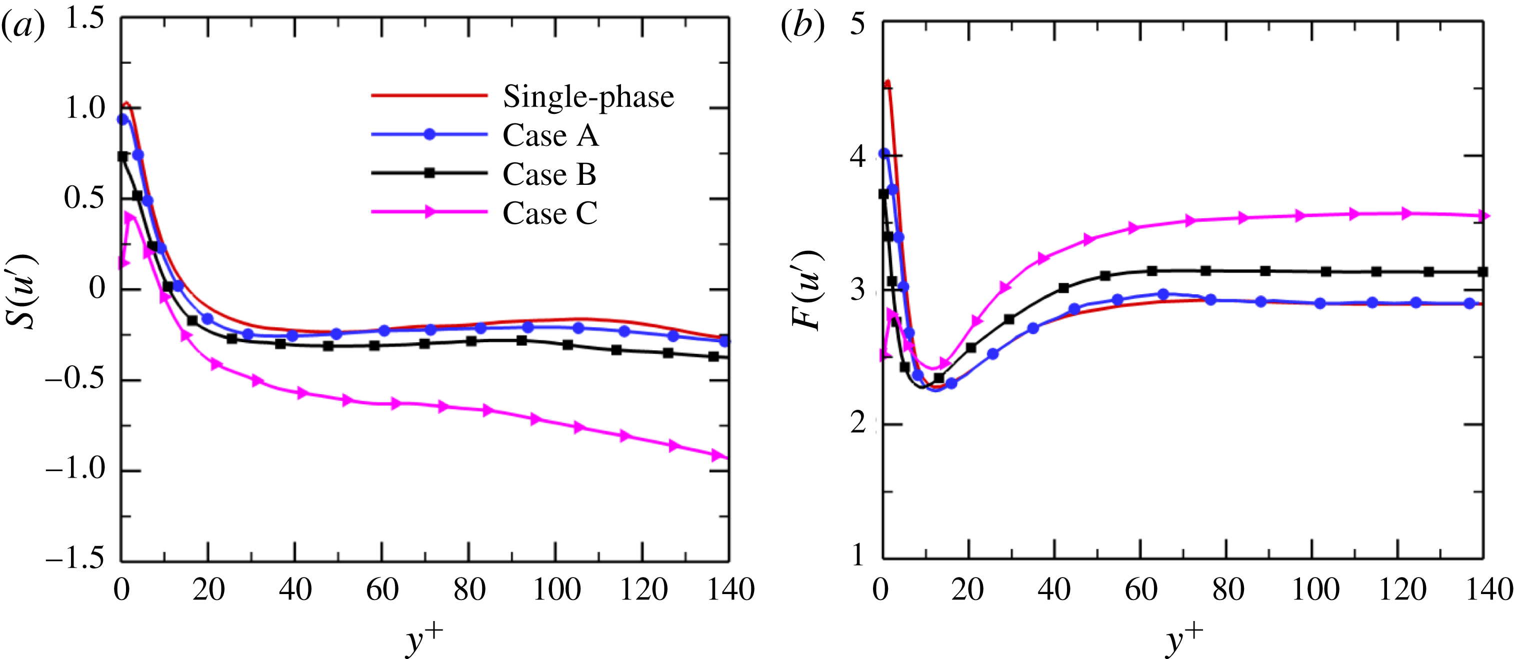
Higher-order moments of velocity fluctuations plotted versus the inner wall coordinate
 $y^{+}$
at
 $x=4867\unicode[STIX]{x1D703}_{0}$
: (a) skewness factor of streamwise velocity fluctuation,
 $S(u^{\prime })$
; (b) flatness factor of streamwise velocity fluctuation,
 $F(u^{\prime })$
.

3.4 Higher-order statistics
The higher-order statistics of the velocity are likely to be more sensitive to the presence of particles than the second-order statistics owing to their greater degree of nonlinearity. In this subsection, we examine the effects of particles on higher-order turbulent statistics. The skewness and flatness factors for the streamwise velocity fluctuation,
 $$\begin{eqnarray}\displaystyle & \displaystyle S(u^{\prime })=\frac{\overline{u^{\prime 3}}}{(\overline{u^{\prime 2}})^{3/2}}, & \displaystyle\end{eqnarray}$$
 $$\begin{eqnarray}\displaystyle & \displaystyle F(u^{\prime })=\frac{\overline{u^{\prime 4}}}{(\overline{u^{\prime 2}})^{2}}, & \displaystyle\end{eqnarray}$$
 $St$
and mass loading
 $\unicode[STIX]{x1D6F7}_{m}$
. As indicated in figure 14(a), the inertial particles produce a noticeable decrease in the skewness factor of streamwise velocity fluctuation,
 $S(u^{\prime })$
, which is consistent with the numerical results of Pan & Banerjee (Reference Pan and Banerjee1996). Moreover, the level of reduction increases monotonically with particle Stokes number and mass loading. In other words, the particles with
 $d_{p}<\unicode[STIX]{x1D702}$
tend to attenuate the positive streamwise velocity fluctuations
 $u^{\prime }$
in the vicinity of the wall. On the other hand, according to Kim et al. (Reference Kim, Moin and Moser1987), most of the large values of
 $u^{\prime }$
in the near-wall region are due to the sweep effect. This means that the small solid particles tend to dampen the sweep motions. Given that the sweep motions dominate the near-wall Reynolds stress (Robinson Reference Robinson1991), we can thus infer that the presence of small particles suppresses the Reynolds shear stress, which is consistent with the quantitative results shown in figure 10(d).
As far as the flatness profile
 $F(u^{\prime })$
is concerned, we can see from figure 14(b) that for both the single-phase and particle-laden flows, the locations at which the minima of
 $F(u^{\prime })$
occur correspond to the locations of the maximum streamwise velocity fluctuations. In the vicinity of the wall, the particles clearly reduce the flatness factor
 $F(u^{\prime })$
. Far away from the wall, however, the flatness factor
 $F(u^{\prime })$
increases as the particle inertia and mass loading increase. This indicates that in the outer region, the streamwise velocity fluctuations become more intermittent under the effect of the particles, while the reverse is true in the very-near-wall region.
3.5 Mean momentum balance
The dynamical mechanisms of the mean momentum balance in a single-phase turbulent boundary layer have been studied previously (Klewicki, Ebner & Wu Reference Klewicki, Ebner and Wu2011; Sayadi et al. Reference Sayadi, Hamman and Moin2013). In this subsection, we investigate the effect of the presence of particles on the mean momentum balance in particle-laden flows. Accordingly, we consider the inner normalized mean streamwise momentum transport equation for zero-pressure-gradient particle-laden boundary layer flow:
 $$\begin{eqnarray}-\!\left(\bar{u}^{+}\frac{\unicode[STIX]{x2202}\bar{u}^{+}}{\unicode[STIX]{x2202}x^{+}}+\bar{v}^{+}\frac{\unicode[STIX]{x2202}\bar{u}^{+}}{\unicode[STIX]{x2202}y^{+}}\right)+\frac{\unicode[STIX]{x2202}^{2}\bar{u}^{+}}{\unicode[STIX]{x2202}y^{+2}}-\frac{\unicode[STIX]{x2202}\overline{u^{\prime }v^{^{\prime }}}^{\,+}}{\unicode[STIX]{x2202}y^{+}}+\bar{f}_{x}^{+}=0,\end{eqnarray}$$
where the terms on the left-hand side represent different physical mechanisms: the first term is the negative mean advection; the second term,
 $\unicode[STIX]{x2202}^{2}\bar{u}^{+}/\unicode[STIX]{x2202}y^{+2}$
, is the gradient of the mean viscous stress; the third term,
 $-\unicode[STIX]{x2202}\overline{u^{\prime }v^{^{\prime }}}^{\,+}/\unicode[STIX]{x2202}y^{+}$
, is the gradient of the Reynolds stress; and the last term,
 $\bar{f}_{x}^{+}$
, denotes the streamwise component of the mean particle-to-fluid feedback force.
In order to elucidate the mean momentum transport, it is useful to compare the relative magnitudes of the budget terms in the mean momentum balance equation. Figure 15 presents the budget terms in (3.8) for the single-phase and particle-laden cases in the near-wall region at
 $x=4867\unicode[STIX]{x1D703}_{0}$
. For single-phase flow, the Reynolds stress gradient and the mean viscous stress gradient dominate the balance equation in the turbulent region, while the mean advection is negligible. This is consistent with the DNS results of Klewicki et al. (Reference Klewicki, Ebner and Wu2011) and Sayadi et al. (Reference Sayadi, Hamman and Moin2013). For the particle-laden flows, however, the absolute value of the gradient of the viscous stress is increased, whereas the gradient of the Reynolds stress is reduced, and the effect is intensified with increasing particle mass loading. This is due to the fact that the mean velocity gradient
 $\text{d}\bar{u}/\text{d}y$
is enhanced by the solid particles but decreases monotonically in the wall-normal direction, while the Reynolds stress
 $-\overline{u^{\prime }v^{\prime }}$
is reduced but increases monotonically along the wall-normal direction in the very-near-wall region. Since the Reynolds stress gradient cannot balance the viscous stress gradient in the particle-laden flows, it is expected that as the particle mass loading and Stokes number increase, the mean streamwise feedback force
 $\bar{f}_{x}$
will play an increasingly significant role in the momentum balance equation. It is noteworthy that the mean viscous stress gradient
 $\unicode[STIX]{x2202}^{2}\bar{u}^{+}/\unicode[STIX]{x2202}y^{+2}$
at the wall is no longer zero for the cases with higher mass loading
 $\unicode[STIX]{x1D6F7}_{m}=1.0$
, and this phenomenon becomes more pronounced with increasing Stokes number. The distinct negative value of
 $\unicode[STIX]{x2202}^{2}\bar{u}^{+}/\unicode[STIX]{x2202}y^{+2}$
at the wall is probably associated with the reaction force from the particles onto the fluid and will be discussed below.
Budget terms in (3.8) at the turbulent station
 $x=4867\unicode[STIX]{x1D703}_{0}$
for the single-phase case (lines without symbols) and the particle-laden cases: A (lines with circles), B (lines with squares) and C (lines with triangles). Solid lines, Reynolds stress gradient; dashed lines, viscous stress gradient; dashed-single-dotted lines, advection; dashed-double-dotted lines, streamwise feedback force.

The evolutions of each term in (3.8) are depicted in figures 16–18 for cases A, B and C respectively, ranging from the laminar region to the fully developed turbulent region. The particle mass loading and Stokes number have remarkable impacts on the momentum balance. In the laminar region, the mean advection is balanced by the mean viscous stress gradient, whereas the Reynolds stress gradient is negligible for case A, with lower mass loading
 $\unicode[STIX]{x1D6F7}_{m}=0.1$
. With increasing particle mass loading and Stokes number, however, the mean streamwise force becomes an important source of momentum. For cases B and C, the mean advection and mean streamwise force dominate the mean viscous stress gradient.
As the streamwise distance increases, the mean advection term gradually decreases, while the Reynolds stress gradient term rapidly increases and becomes more and more important during the transition stage. At the location where transition is complete (
 $x=3400\unicode[STIX]{x1D703}_{0}$
in case A,
 $x=2260\unicode[STIX]{x1D703}_{0}$
in case B and
 $x=4160\unicode[STIX]{x1D703}_{0}$
in case C), the Reynolds and viscous stress gradients reach maxima in the near-wall region. Far away from the wall, the mean advection and the Reynolds stress gradient are essentially in balance, whereas the mean viscous stress gradient and the streamwise feedback force are vanishingly small; see, e.g., figures 16(f) and 17(f).
In the turbulent region, the Reynolds stress gradient and the mean streamwise force positively sum to balance the negative viscous stress gradient. The mean advection term is much smaller than the other terms and can therefore be ignored. Although the mean viscous stress gradient at the wall is zero in the single-phase flow, as mentioned previously, the presence of particles fundamentally alters that. At higher mass loading and larger Stokes number (case C), a large negative value of the viscous stress gradient is obtained quite close to the wall in the transitional and turbulent regions, which is balanced by the positive streamwise feedback force. Given that the maximum particle number density is observed at the wall (figure 3), we can infer that the particle–fluid interactions are most prominent in the close vicinity of the wall, which produces a large positive reaction force exerted by the particles on the fluid and in turn induces a negative viscous stress gradient. The particle–fluid interactions will be studied in detail in § 5 by investigating kinetic energy transfer between the solid particles and fluid turbulence.
4 Modulation of turbulent coherent structures
In addition to modulation of the mean and fluctuating statistics of the turbulence, the presence of inertial solid particles also affects turbulent coherent structures. Coherent structures are of great importance in turbulent boundary layer flow. Although turbulent coherent structures have been investigated numerically and experimentally for many years, as already mentioned in § 1, there is limited research reported about the modulation of coherent structures by particles in the literature (Dritselis & Vlachos Reference Dritselis and Vlachos2008, Reference Dritselis and Vlachos2011; Li et al. Reference Li, Wang, Liu, Chen and Zheng2012). In this section, we focus on the effect of inertial particles on near-wall coherent structures by examining the instantaneous flow fields and their statistical properties.
Evolution of the terms in (3.8) for case A at (a)
 $x=300\unicode[STIX]{x1D703}_{0}$
, (b)
 $x=450\unicode[STIX]{x1D703}_{0}$
, (c)
 $x=800\unicode[STIX]{x1D703}_{0}$
, (d)
 $x=1160\unicode[STIX]{x1D703}_{0}$
, (e)
 $x=1500\unicode[STIX]{x1D703}_{0}$
, (f)
 $x=2260\unicode[STIX]{x1D703}_{0}$
, (g)
 $x=3400\unicode[STIX]{x1D703}_{0}$
, (h)
 $x=5000\unicode[STIX]{x1D703}_{0}$
, (i)
 $x=6000\unicode[STIX]{x1D703}_{0}$
; ——, Reynolds stress gradient; – ⋅ – ⋅ –, negative advection; - - - -, viscous stress gradient; –▪–, streamwise feedback force.

Evolution of the terms in (3.8) for case B at (a)
 $x=300\unicode[STIX]{x1D703}_{0}$
, (b)
 $x=450\unicode[STIX]{x1D703}_{0}$
, (c)
 $x=800\unicode[STIX]{x1D703}_{0}$
, (d)
 $x=1160\unicode[STIX]{x1D703}_{0}$
, (e)
 $x=1500\unicode[STIX]{x1D703}_{0}$
, (f)
 $x=2260\unicode[STIX]{x1D703}_{0}$
, (g)
 $x=3400\unicode[STIX]{x1D703}_{0}$
, (h)
 $x=5000\unicode[STIX]{x1D703}_{0}$
, (i)
 $x=6000\unicode[STIX]{x1D703}_{0}$
; ——, Reynolds stress gradient; – ⋅ – ⋅ –, negative advection; - - - -, viscous stress gradient; –▪–, streamwise feedback force.

Evolution of the terms in (3.8) for case C at (a)
 $x=300\unicode[STIX]{x1D703}_{0}$
, (b)
 $x=800\unicode[STIX]{x1D703}_{0}$
, (c)
 $x=1500\unicode[STIX]{x1D703}_{0}$
, (d)
 $x=2260\unicode[STIX]{x1D703}_{0}$
, (e)
 $x=3400\unicode[STIX]{x1D703}_{0}$
, (f)
 $x=4160\unicode[STIX]{x1D703}_{0}$
, (g)
 $x=5000\unicode[STIX]{x1D703}_{0}$
, (h)
 $x=6000\unicode[STIX]{x1D703}_{0}$
, (i)
 $x=6500\unicode[STIX]{x1D703}_{0}$
; ——, Reynolds stress gradient; – ⋅ – ⋅ –, negative advection; - - - -, viscous stress gradient; –▪–, streamwise feedback force.

4.1 Instantaneous flow field visualizations
Figure 19 presents instantaneous snapshots of three-dimensional vortical structures inside the turbulent boundary layer for the single-phase flow and the particle-laden flow of case B. Here, the vortical structures, coloured by local streamwise velocity, are identified using the isosurfaces of the second invariant of the instantaneous velocity gradient tensor (Hunt, Wray & Moin Reference Hunt, Wray and Moin1988). It should be noted that the solid particles in case B are indicated by small white spheres in this figure. It is apparent that the turbulent boundary layers are dominated by hairpin vortices in both the single-phase and particle-laden flows. However, the vortical structures become less organized in the particle-laden flow owing to disturbance by the particles.
Instantaneous isosurfaces of the second invariant of the instantaneous velocity gradient tensor in the turbulent region: (a) single-phase flow; (b) particle-laden flow (case B). It should be noted that the vortical structures are coloured by local streamwise velocity and that the particles are indicated here by small white spheres.

The contours of the instantaneous streamwise fluctuating velocity
 $u^{\prime }$
in the near-wall region at
 $y^{+}=15$
are displayed in figure 20. The alternating high- and low-speed streaks are clearly visible in the wall-bounded flows. It can be seen that the particles appear to reduce the regions of high-speed fluid, while increasing the number of streamwise-elongated streaks of low-speed fluid. Moreover, the near-wall low-speed streaky structures become more intense under the effect of the particles.
Distribution of instantaneous streamwise fluctuating velocity
 $u^{\prime }$
in the near-wall region at
 $y^{+}=15$
: (a) single-phase flow; (b) particle-laden flow (case B). Red indicates high positive values of
 $u^{\prime }$
and blue high negative values.

4.2 Two-point correlation
In wall-bounded flows, the spatial two-point correlations of velocity fluctuations are usually used to estimate the averaged length scales of typical structures (Kim et al. Reference Kim, Moin and Moser1987; Sayadi et al. Reference Sayadi, Hamman and Moin2013). In order to gain further understanding of the effect of particles on turbulent coherent structures, figure 21 shows the spanwise two-point correlations of the streamwise, wall-normal and spanwise velocity fluctuations,
 $$\begin{eqnarray}\displaystyle & \displaystyle R_{u^{\prime }u^{\prime }}(\unicode[STIX]{x0394}z)=\frac{\overline{u^{\prime }(x,y,z,t)u^{\prime }(x,y,z+\unicode[STIX]{x0394}z,t)}}{\overline{u^{\prime }(x,y,z,t)u^{\prime }(x,y,z,t)}}, & \displaystyle\end{eqnarray}$$
 $$\begin{eqnarray}\displaystyle & \displaystyle R_{v^{\prime }v^{\prime }}(\unicode[STIX]{x0394}z)=\frac{\overline{v^{\prime }(x,y,z,t)v^{\prime }(x,y,z+\unicode[STIX]{x0394}z,t)}}{\overline{v^{\prime }(x,y,z,t)v^{\prime }(x,y,z,t)}}, & \displaystyle\end{eqnarray}$$
 $$\begin{eqnarray}\displaystyle & \displaystyle R_{w^{\prime }w^{\prime }}(\unicode[STIX]{x0394}z)=\frac{\overline{w^{\prime }(x,y,z,t)w^{\prime }(x,y,z+\unicode[STIX]{x0394}z,t)}}{\overline{w^{\prime }(x,y,z,t)w^{\prime }(x,y,z,t)}}, & \displaystyle\end{eqnarray}$$
 $R_{u^{\prime }u^{\prime }}$
. The spanwise separation at which the minimum of
 $R_{u^{\prime }u^{\prime }}$
occurs corresponds approximately to half the mean spacing of the streaks. In the single-phase flow, as shown in figure 21(a), the minimum of
 $R_{u^{\prime }u^{\prime }}$
at
 $y^{+}=5$
is negative and occurs at
 $\unicode[STIX]{x0394}z^{+}\approx 50$
, indicating that the wall-layer streaks have a mean spacing of approximately 100 in viscous units, which is consistent with the numerical results of Kim et al. (Reference Kim, Moin and Moser1987) and the experimental data of Kline et al. (Reference Kline, Reynolds, Schraub and Runstadler1967). In case A, with lower mass loading
 $\unicode[STIX]{x1D6F7}_{m}=0.1$
, no pronounced change is observed in the profile of
 $R_{u^{\prime }u^{\prime }}$
. As the particle mass loading increases, the particles with smaller Stokes number
 $St=10$
(case B) reduce the streak spacing while the larger particles with
 $St=50$
(case C) widen it. In the logarithmic layer at
 $y^{+}=80$
, the separation distances are obviously increased and more than twice as large as those in the wall region, for both the single-phase and particle-laden flows (figure 21
b).
Kim et al. (Reference Kim, Moin and Moser1987) suggested that the separation of the distinct negative minimum of
 $R_{v^{\prime }v^{\prime }}$
corresponds to the mean diameter of the near-wall streamwise vortices. From the profiles of
 $R_{v^{\prime }v^{\prime }}$
(figure 21
c), it is clear that the presence of particles with larger inertia
 $St=50$
increases the mean diameter of the streamwise vortices, while the particles with smaller inertia
 $St=10$
do not produce any noticeable change in vortex size, even though the particle mass loading in case B is as high as in case C. It is interesting to observe that the minimum of
 $R_{v^{\prime }v^{\prime }}$
gradually increases with increasing particle Stokes number and mass loading. This indicates that the turbulent coherent structures are strongly affected by the solid particles and become less ordered at larger particle Stokes number and higher mass loading, which is consistent with the qualitative observations in figure 19.
The spanwise separation of the minimum of
 $R_{w^{\prime }w^{\prime }}$
usually corresponds to the mean spacing between pairs of counter-rotating streamwise vortices in the near-wall region. In the present study, the particles with smaller inertia have no significant influence on the mean spacing of the streamwise vortices, irrespective of particle mass loading, as can be seen from figure 21(e). Nevertheless, the particles with larger inertia slightly increase the mean spacing of the near-wall streamwise vortices. Further away from the wall, at
 $y^{+}=80$
, we observe in figures 21(d) and 21(f) that the local sharp minima of
 $R_{v^{\prime }v^{\prime }}$
and
 $R_{w^{\prime }w^{\prime }}$
tend to disappear. Therefore, we can conclude that the larger particles with
 $St=50$
increase the diameter and mean spacing of the streamwise vortices, while the smaller particles with
 $St=10$
have no remarkable effect on them.
Spanwise two-point correlations of the velocity fluctuations in the turbulent region at
 $x=4867\unicode[STIX]{x1D703}_{0}$
: (a)
 $R_{u^{\prime }u^{\prime }}$
at
 $y^{+}=5$
; (b)
 $R_{u^{\prime }u^{\prime }}$
at
 $y^{+}=80$
; (c)
 $R_{v^{\prime }v^{\prime }}$
at
 $y^{+}=5$
; (d)
 $R_{v^{\prime }v^{\prime }}$
at
 $y^{+}=80$
; (e)
 $R_{w^{\prime }w^{\prime }}$
at
 $y^{+}=5$
; (f)
 $R_{w^{\prime }w^{\prime }}$
at
 $y^{+}=80$
.

Probability density functions of velocity fluctuations in the turbulent region at
 $x=4867\unicode[STIX]{x1D703}_{0}$
: (a) p.d.f.
 $(u^{\prime })$
at
 $y^{+}=5$
; (b) p.d.f.
 $(u^{\prime })$
at
 $y^{+}=80$
; (c) p.d.f.
 $(v^{\prime })$
at
 $y^{+}=5$
; (d) p.d.f.
 $(v^{\prime })$
at
 $y^{+}=80$
; (e) p.d.f.
 $(w^{\prime })$
at
 $y^{+}=5$
; (f) p.d.f.
 $(w^{\prime })$
at
 $y^{+}=80$
.

4.3 Probability density functions
Figure 22(a) shows the probability density function (p.d.f.) of the streamwise velocity fluctuation in the near-wall region at
 $y^{+}=5$
. In the single-phase flow, the peak location of the p.d.f. of the streamwise velocity fluctuations, p.d.f.
 $(u^{\prime })$
, shifts towards negative values and the positive tail is larger than the negative tail. This is consistent with the well-known characteristic of the high- and low-speed streaks, namely that the regions of high-speed fluid tend to be shorter and more intense than the elongated streaks of low-speed fluid (Robinson Reference Robinson1991). It is interesting to note that the peaks of p.d.f.
 $(u^{\prime })$
in the particle-laden flows are shifted slightly towards zero, indicating that the presence of particles shortens the length of the low-speed streak. On the other hand, both the positive and the negative tails extend longer, with the effect being more pronounced at higher mass loading
 $\unicode[STIX]{x1D6F7}_{m}=1.0$
. This implies that the high- and low-speed streaks in the particle-laden flows appear to be more intense than in the unladen flow, resulting in augmentation of the streamwise velocity fluctuations in the vicinity of the wall (figure 10
a). Given that the streamwise vortices create the wall-layer streaks, we can therefore infer that the presence of small solid particles enhances the strength of the near-wall streamwise vortices. Far away from the wall, at
 $y^{+}=80$
, p.d.f.
 $(u^{\prime })$
in the single-phase flow tends to be symmetric about zero, while the negative tails are lengthened in the particle-laden flows, see figure 22(b). In addition, the peak of p.d.f.
 $(u^{\prime })$
for case C in the logarithmic layer (
 $y^{+}=80$
) is moved towards positive values, in contrast to that in the viscous sublayer (
 $y^{+}=5$
).
With regard to the p.d.f. of the wall-normal velocity fluctuation at
 $y^{+}=5$
, as shown in figure 22(c), the single-phase p.d.f. is approximately symmetric about zero. On the contrary, the profiles of p.d.f.
 $(v^{\prime })$
are no longer symmetric about zero in the particle-laden simulations. The presence of particles with smaller inertia
 $St=10$
shortens the positive tail but lengthens the negative one. In the region far from the wall with
 $y^{+}=80$
, however, both the positive and the negative tails are significantly reduced, and the degree of reduction increases with particle Stokes number and mass loading, leading to an obvious attenuation of the wall-normal turbulence intensity (figure 10
b). The p.d.f. distributions of the spanwise velocity fluctuations, shown in figures 22(e) and 22(f), exhibit similar characteristics to p.d.f.
 $(v^{\prime })$
. For the cases with higher mass loading
 $\unicode[STIX]{x1D6F7}_{m}=1.0$
, the presence of particles leads to an increase in the size of the peaks in p.d.f.
 $(w^{\prime })$
and shortens both the negative and the positive tails at
 $y^{+}=80$
, with these effects being intensified as the particle inertia increases. As a result, the spanwise velocity fluctuations are substantially suppressed, as seen in figure 10(c).
5 Kinetic energy transfer between particles and fluid
In order to explain, from a physical viewpoint, the mechanisms of turbulence modulation in the presence of small solid particles, we investigate the transfer of kinetic energy between the particle and fluid phases in particle-laden flows. The relationship between the work performed by the particles on the fluid and that performed by the fluid on the particles is examined in detail in this section.
The rate of mechanical work done by a force, i.e. the power, is the scalar product of the force and velocity vectors. In the present simulations, the rate of work exerted by the local fluid on particle
 $n$
can be written as
 $$\begin{eqnarray}P^{p}=\boldsymbol{F}^{n}\boldsymbol{\cdot }\boldsymbol{u}_{p}^{n},\end{eqnarray}$$
where
 $\boldsymbol{F}^{n}$
denotes the total force acting on particle
 $n$
and
 $\boldsymbol{u}_{p}^{n}$
is the velocity vector of that particle. According to Newton’s third law, the feedback force on the local fluid from the particle
 $n$
is therefore
 $-\boldsymbol{F}^{n}$
. Hence, the rate of work done by particle
 $n$
on the local fluid is given by
 $$\begin{eqnarray}P^{f}=-\boldsymbol{F}^{n}\boldsymbol{\cdot }\boldsymbol{u}_{f}^{n},\end{eqnarray}$$
where
 $\boldsymbol{u}_{f}^{n}$
is the local fluid velocity at the centre of particle
 $n$
. It is important to note that a positive
 $P^{f}$
or a negative
 $P^{p}$
indicates that the particle exerts work on the fluid, with kinetic energy being transferred from particle to fluid, while a negative
 $P^{f}$
or a positive
 $P^{p}$
means that the fluid performs work on the particle, with kinetic energy being transferred from fluid to particle. The sum
 $$\begin{eqnarray}\unicode[STIX]{x1D700}^{p}=P^{f}+P^{p}\end{eqnarray}$$
represents the net gain or loss of kinetic energy in a particle-laden flow.
Figure 23(a) reports the mean power exchange between particles and fluid in the turbulent region at
 $x=4867\unicode[STIX]{x1D703}_{0}$
for case C. It should be noticed that the mean power is evaluated by first summing over all the particles in each control volume, and then averaging in time and in the homogeneous spanwise direction. Near the wall, the mean power transferred from fluid to particles,
 $\overline{P^{p}}$
, is negative, whereas the power received by the fluid from the particles,
 $\overline{P^{f}}$
, is positive, indicating that the particles perform work on the fluid in the near-wall region. It is noteworthy that the sum of
 $\overline{P^{p}}$
and
 $\overline{P^{f}}$
is not equal to zero but a slightly negative value,
 $\overline{\unicode[STIX]{x1D700}^{p}}$
, in the vicinity of the wall. This implies that the exchange of kinetic energy between the particle and fluid phases is unbalanced and the interactions between the two phases lead to an extra dissipation of the kinetic energy, i.e. particle-induced dissipation
 $\overline{\unicode[STIX]{x1D700}^{p}}$
. Since (5.3) can be expressed as
 $\unicode[STIX]{x1D700}^{p}=\boldsymbol{F}\boldsymbol{\cdot }(\boldsymbol{u}_{p}-\boldsymbol{u}_{f})$
, it can be inferred that the interphase energy exchange is caused by the velocity difference between the particles and the fluid.
To provide further insight into the energy transfer process, figure 23(b–d) shows the components of the mean power in the streamwise, wall-normal and spanwise directions. It is clear that the streamwise component of the mean power dominates the energy transfer, while the mean powers in the wall-normal and spanwise directions have lower-order effects on the kinetic energy exchange between particles and fluid.
Mean power exchange between particles and fluid and the particle-induced dissipation at
 $x=4867\unicode[STIX]{x1D703}_{0}$
for case C: (a) total mean power; (b) streamwise component of the mean power; (c) wall-normal component of the mean power; (d) spanwise component of the mean power. It should be noted that all of the terms are multiplied by
 $10^{5}$
.

In order to investigate whether the mean part or the fluctuating part of the mean power is more important, the Reynolds decomposition, in which all quantities are written as sums of mean and fluctuating parts, is introduced here. Thus, the mean power
 $\overline{P^{p}}$
is decomposed into mean and fluctuating parts as follows:
 $$\begin{eqnarray}\overline{P^{p}}=\overline{\boldsymbol{F}\boldsymbol{\cdot }\boldsymbol{u}_{p}}=\overline{(\bar{\boldsymbol{F}}+\boldsymbol{F}^{\prime })\boldsymbol{\cdot }(\bar{\boldsymbol{u}}_{p}+\boldsymbol{u}_{p}^{\prime })}=\bar{\boldsymbol{F}}\boldsymbol{\cdot }\bar{\boldsymbol{u}}_{p}+\overline{\boldsymbol{F}^{\prime }\boldsymbol{\cdot }\boldsymbol{u}_{p}^{\prime }},\end{eqnarray}$$
where
 $\boldsymbol{F}^{\prime }$
is the fluctuating part of the total force on the particles,
 $\boldsymbol{u}_{p}^{\prime }$
is the fluctuating part of the velocity vector of the particles, and
 $\bar{\boldsymbol{F}}$
and
 $\bar{\boldsymbol{u}}_{p}$
are the corresponding mean parts of the total force and the particle velocity vector respectively. The first and second terms on the right-hand side of (5.4) represent the mean and fluctuating parts respectively of the power
 $\overline{P^{p}}$
. Similarly, the mean power
 $\overline{P^{f}}$
can be decomposed as follows:
 $$\begin{eqnarray}\overline{P^{f}}=\overline{-\boldsymbol{F}\boldsymbol{\cdot }\boldsymbol{u}_{f}}=-\overline{(\bar{\boldsymbol{F}}+\boldsymbol{F}^{\prime })\boldsymbol{\cdot }(\bar{\boldsymbol{u}}_{f}+\boldsymbol{u}_{f}^{\prime })}=-(\bar{\boldsymbol{F}}\boldsymbol{\cdot }\bar{\boldsymbol{u}}_{f}+\overline{\boldsymbol{F}^{\prime }\boldsymbol{\cdot }\boldsymbol{u}_{f}^{\prime }}),\end{eqnarray}$$
where the equation can be interpreted in a similar manner to (5.4).
Mean and fluctuating parts of the mean power for case C: (a) mean part in the streamwise direction; (b) fluctuating part in the streamwise direction; (c) fluctuating part in the wall-normal direction; (d) fluctuating part in the spanwise direction. It should be noted that all of the terms are multiplied by
 $10^{5}$
.

Figure 24 shows the mean and fluctuating parts of the mean power in the streamwise, wall-normal and spanwise directions. It can be seen that in the streamwise direction, both the mean and the fluctuating parts of the power are responsible for kinetic energy transfer. The profiles in figure 24(a) indicate that the fluid gains mean kinetic energy from the particles in the vicinity of the wall and thus the mean streamwise fluid velocity is increased significantly (figure 7).
Although the kinetic energy transfer caused by the mean motion in the streamwise direction is larger than that due to streamwise velocity fluctuations, the extra energy dissipation stems mainly from the fluctuating velocity field. On the other hand, the pronounced positive value of
 $\overline{P_{x,fluc}^{f}}$
in figure 24(b) indicates that turbulent kinetic energy is transferred from inertial particles to fluid, which can probably explain the slight augmentation of the streamwise turbulence intensity in the near-wall region (figure 10
a). Therefore, we can infer that the extra energy dissipation in the streamwise direction arises mainly from the particle fluctuations. In the wall-normal and spanwise directions, however, the mean parts of the mean powers can be neglected in comparison with the fluctuating parts, i.e.
 $\overline{P_{y}}\approx \overline{P_{y,fluc}}$
and
 $\overline{P_{z}}\approx \overline{P_{z,fluc}}$
, which suggests that only the fluctuating parts are responsible for the energy transfer in the directions perpendicular to the mean flow. The significantly negative values of
 $\overline{P_{y,fluc}^{f}}$
and
 $\overline{P_{z,fluc}^{f}}$
imply that the fluid phase loses turbulent kinetic energy. It is interesting to note, however, that the particle phase could not gain energy from the fluid, since
 $\overline{P_{y,fluc}^{p}}$
and
 $\overline{P_{z,fluc}^{p}}$
are both almost zero. As a result, the turbulent kinetic energy coming from the fluid is dissipated rather than being transferred to the particles. We can therefore conclude that the attenuation of turbulence intensities in the wall-normal and spanwise directions, as shown in figures 10(b) and 10(c), can be explained in terms of the extra energy dissipation due to particle–fluid interactions.
6 Concluding remarks
Direct numerical simulation of particle-laden flows in a spatially developing flat-plate boundary layer has been performed using the two-way coupled Eulerian–Lagrangian point-particle approach. The focus has been on dilute flows in which particle–particle interactions are not taken into account. Three different cases have been simulated and compared in order to investigate the effects of particle Stokes number and mass loading on turbulence modulation.
The results indicate that the presence of inertial particles leads to an increase in the mean streamwise fluid velocity. As a consequence, the boundary layer integral parameters are decreased, while the skin-friction drag is increased. Moreover, these effects are intensified as the particle Stokes number and mass loading increase. The streamwise turbulence intensity is slightly augmented in the very-near-wall region whereas it is attenuated in the outer layer. However, the small inertial particles significantly suppress the Reynolds stress and the velocity fluctuations in the wall-normal and spanwise directions, with the degree of suppression increasing monotonically with particle Stokes number and mass loading.
With regard to the effect of solid particles on near-wall coherent structures, it is found that the diameter and mean spacing of streamwise vortices are increased in the presence of particles with larger inertia, but are not affected significantly by smaller particles. The wall-layer streak spacing is slightly decreased by the smaller particles whereas it is increased by the larger ones. As the particle Stokes number and mass loading increase, turbulent coherent structures become less organized due to the strong interactions between particles and fluid turbulence.
In the final part of this paper, we have provided a detailed analysis of the exchange of kinetic energy between the fluid and the particles, in an attempt to elucidate the mechanism of turbulence modulation. In the streamwise direction, the energy from the particles is partly transferred to the fluid and partly dissipated in the vicinity of the wall. As a consequence, the mean streamwise fluid velocity is enhanced, resulting in an increase in the skin-friction coefficient and decreases in the boundary layer integral parameters. In addition, the enhancement of the streamwise velocity fluctuations in the near-wall region is probably due to the fact that the particles perform work on the local fluid, which thus receives turbulent kinetic energy from the particles. In the directions perpendicular to the mean flow, the turbulent kinetic energy coming from the fluid is not transferred to the particles but rather is dissipated, leading to attenuation of the turbulent velocity fluctuations in the wall-normal and spanwise directions.
It is worth commenting here that the turbulent kinetic energy is dissipated by two different mechanisms: viscous dissipation occurring throughout the fluid phase and particle-induced dissipation due to interactions between particles and fluid turbulence. On the one hand, the difference between the production rate and the viscous dissipation rate of the turbulent kinetic energy is decreased owing to the presence of particles. On the other hand, the particle-induced extra dissipation causes a net loss of turbulent kinetic energy. We can therefore conclude that the combination of reduced energy production, viscous dissipation and particle-induced dissipation ultimately leads to strong damping of the turbulent kinetic energy.
Acknowledgement
This work is supported by the National Natural Science Foundation of China (no. 51136006). We are grateful for this.