





Introduction
Interfaces between varying boundary conditions are critical to ice-sheet dynamics. For example, the organization of ice flow into ice streams, which serve as fast flowing conduits through which Antarctic ice is rapidly transported seaward (e.g., Bindschadler and Vornberger, Reference Bindschadler and Vornberger1998; Hulbe and Fahnestock, Reference Hulbe and Fahnestock2007; Rignot and others, Reference Rignot, Mouginot and Scheuchl2011), is dependent on the dynamics associated with a transition in basal boundary condition (Jacobson and Raymond, Reference Jacobson and Raymond1998; Suckale and others, Reference Suckale, Platt, Perol and Rice2014; Mantelli and others, Reference Mantelli, Haseloff and Schoof2019). The flux of ice through the grounding line (e.g., off the edge of the continent to form floating ice shelves in the ocean) is critically dependent on the dynamics at the basal boundary transition of the grounding line (Weertman, Reference Weertman1974; Chugunov and Wilchinsky, Reference Chugunov and Wilchinsky1996; Schoof, Reference Schoof2007a). Another such glacial interface is a seasonally occurring feature of the Greenland ice sheet (GrIS): rapid spatially finite injections of surface meltwater to the ice-bed interface from the drainage of supraglacial lakes through the ice column (e.g., Das and others, Reference Das2008; Tsai and Rice, Reference Tsai and Rice2010; Stevens and others, Reference Stevens2015).
During the summer months (June–September), the GrIS ice-bed interface becomes partially lubricated by surface meltwater, which penetrates the ice column via surface-to-bed pathways, such as moulins and hydrofracture-driven lake drainages (HLDs) (e.g.,
Alley and others, Reference Alley, Dupont, Parizek and Anandakrishnan2005; Das and others, Reference Das2008). These spatially finite injections of meltwater reduce the friction between the ice and bed below, leading to a transient acceleration of the overlying ice (Joughin and others, Reference Joughin2013; Stevens and others, Reference Stevens2016). In many cases, the resulting induced stresses are sufficient to trigger further HLD events, delivering further lubricating water to the bed (Das and others, Reference Das2008; Stevens and others, Reference Stevens2015; Christoffersen and others, Reference Christoffersen, Bougamont, Hubbard, Doyle, Grigsby and Pettersson2018; Poinar and Andrews, Reference Poinar and Andrews2021). These rapid HLD events can deliver large volumes of water ( $\sim5\times10^7\,\textrm{m}^3$) to the bed (Fitzpatrick and others, Reference Fitzpatrick2014), which form spatially finite blisters of diameter on the order of several ice thicknesses beneath the ice, reducing the effective pressure (ice overburden minus basal water pressure) over that area (e.g.,
Lai and others, Reference Lai2021; Stevens and others, Reference Stevens2024).
In some cases, multiple neighboring lakes are observed to drain in rapid succession leading to the hypothesis of a domino effect of HLD events, where one lake drainage may trigger another and so on, which could have the capacity to then transiently overwhelm the evacuation capacity of the subglacial hydrological system, leading to increased ice motion (e.g., Christoffersen and others, Reference Christoffersen, Bougamont, Hubbard, Doyle, Grigsby and Pettersson2018). Other studies report that lake drainage cascades are relatively rare compared to one-off drainages, especially over iterative melt seasons (e.g., Lutz and others, Reference Lutz, Tabone, Humbert and Braun2025). Prescience of these dynamics is especially relevant as the presence of lakes is projected to expand inland over the coming decades in response to the warming climate (Leeson and others, Reference Leeson2015; Ignéczi and others, Reference Ignéczi2016; MacFerrin and others, Reference MacFerrin2019). These inland regions are characterized by a subglacial hydrological system, which may be more readily overwhelmed by meltwater injections due to thicker, more gently sloping ice, potentially leading to a lower effective basal friction in response to rapid basal meltwater injection (e.g., HLD) (Chandler and others, Reference Chandler2013; Meierbachtol and others, Reference Meierbachtol, Harper and Humphrey2013; Dow and others, Reference Dow, Kulessa, Rutt, Doyle and Hubbard2014; Doyle and others, Reference Doyle2014). Constraining the structure of the influence one lake drainage has on other lakes in the area via distal stress communication, and how this communication varies across the GrIS, remains a critical challenge. In this study, we aim to investigate the following question: what are the fundamental controls on the magnitude and spatial extent of stress and velocity response to spatially finite basal traction loss?
Our case sits within a broader class of ice flow problems subjected to spatially varying basal boundary conditions. For grounded ice sheets, this type of transition often occurs at the onset (margins) of narrow rapidly moving regions, known as ice streams, which are fed laterally by slower moving ice ridges that are basally frozen. Jacobson and Raymond (Reference Jacobson and Raymond1998) demonstrated the sensitivity of ice stream margin locations to thermo-viscous feedbacks. Haseloff and others (Reference Haseloff, Schoof and Gagliardini2015) derive a boundary layer (BL) description of this lateral transition from slow shear-type to fast plug-type flow, accounting for the role of lateral advection on margin migration. Barcilon and MacAyeal (Reference Barcilon and MacAyeal1993) describe the structure of flow across an along-flow basal condition transition from no-slip to free-slip, work which was extended by Mantelli and others (Reference Mantelli, Haseloff and Schoof2019) and Schoof and Mantelli (Reference Schoof and Mantelli2021) to include the thermomechanical behavior in the associated BLs. The present paper differs in that we discuss a spatially finite region of rapid flow with an upstream transition from slow to fast flow and a downstream transition back to slow flow. We are also interested in systems for which the slippery region is not induced or controlled thermomechanically, but rather simply by the presence of meltwater which can supply sufficient upward pressure on the overlying ice to drastically reduce basal friction, such as the case following a rapid lake drainage (e.g., Lai and others, Reference Lai2021).
Previous attention has been paid to the problem of ice flow over spatially finite basal heterogeneities. Several studies demonstrate steady-state longitudinal transmission of basal heterogeneities (e.g., topography) to be on the order of several ice thicknesses (e.g., Kamb and Echelmeyer, Reference Kamb and Echelmeyer1986; Gudmundsson, Reference Gudmundsson2003; Raymond and Gudmundsson, Reference Raymond and Gudmundsson2005; Sergienko, Reference Sergienko2013; Crozier and others, Reference Crozier, Karlstrom and Yang2018). In particular, Gudmundsson (Reference Gudmundsson2003) investigates surface responses to small amplitude basal slipperiness perturbations, finding regions of extension and compression up- and downstream from the basal heterogeneity, respectively, qualitatively consistent with our findings. Gudmundsson (Reference Gudmundsson2008) uses the shallow-shelf approximation (SSA) to derive analytical transfer functions for small amplitude sinusoidal basal slipperiness perturbations in the Newtonian limit, which imply exponentially decaying spatial responses, consistent with our work. Here, we aim to add to this conversation by posing a boundary value problem for a spatially finite slippery patch, deriving the lengthscale of the BL adjacent to a slippery patch for linear and nonlinear rheology. Using a simple analytical model and scaling arguments, we reveal the dominant relationships between geometrical parameters (ice thickness, slope, patch length) and the resulting stress and velocity perturbations. In this paper, we do not evolve the system forward in time, as the slippery patch-induced stress perturbations are directly relevant for triggering surface fracture and potential subsequent lake drainage cascades. However, long-term impacts of the slippery patch’s annual appearance on ice-sheet dynamics remains an interesting direction for future work.
We begin by presenting our model, which is a simplified representation of the stress coupling from lake drainage-induced basal sliding. We present an analytical model based on the SSA (MacAyeal, Reference MacAyeal1989), as well as two-dimensional (2-D) numerical simulations. We then discuss the implications of this work in the context of GrIS lake drainages under the warming climate before concluding the paper.
Model
We consider an idealized 2-D (along-flow) ice sheet, which is of infinite length, constant thickness and surface slope, and flowing from left to right. In the interior of the domain exists a patch of finite length across which the basal boundary condition is shear-free, that is, a ‘slippery patch’ (Fig. 1). As a further simplification, we consider a depth-averaged version of this model, which admits elementary analytical solutions. We present each of these models, in turn, below. We present this first, before moving to a demonstration of the 2-D system, which is solved numerically.
Schematic of the 2-D flowline model. An ice slab of uniform thickness  $h$ flows over a bed with a spatially finite slippery patch of length
 $\ell$ (orange) where basal friction coefficient
 $C, C_b=0$. Outside the patch, the bed has finite friction
 $C, C_b \gt 0$ set by the sliding ratio
 $\gamma$. Boundary layers form on the up- and downstream edges of the patch, where the flow transitions from free slip to basal friction conditions. The surface slope
 $\alpha$ defines the gravitational driving stress
 $\tau_\mathrm{d}=\rho g h \alpha$. For mathematical convenience, we locate the patch onset at
 $x=0$.

Numerical model (2-D)
We consider a 2-D flowline numerical model. We use the open-source finite element full-Stokes solver Elmer/Ice (Gagliardini and others, Reference Gagliardini2013), with which we conducted a suite of numerical experiments. In particular, we used Elmer/Ice to solve the incompressible Stokes system:
 \begin{equation}
\nabla \cdot \boldsymbol{\sigma} + \rho_\mathrm{i} \mathbf{g} = \mathbf{0}, \qquad \nabla \cdot \mathbf{u} = 0\,,
\end{equation}
where  $\boldsymbol{\sigma}, \rho_\mathrm{i}, \mathbf{g}\ \mathrm{and \,} \mathbf{u}$ are the Cauchy stress tensor, ice density, gravity and velocity field, respectively, and
 $\nabla\cdot$ is the divergence operator. The domain is of length
 $L_x$, and the system is subjected to periodic boundary conditions on both the horizontal (
 $x$) and vertical (
 $z$) components of the velocity field,
 $u(x,z)$ and
 $w(x,z)$, respectively. The simulation mesh is structured with spatially varying horizontal resolution across five zones: fine resolution (10 m) across the center
 $50$ km of the domain, intermediate resolution (100 m) in 50 km zones on both sides adjacent to the central region and coarse resolution (500 m) in the far-field beyond. The mesh is extruded vertically to the ice thickness
 $h$ with 40 vertical levels.
We ran a suite of experiments designed to investigate the relationship between the geometrical parameters of the flow and the resulting stress response. We later compare these empirical relationships to those that arise from the analytical model. To this end, we ran simulations over a range of parameter values for the ice thickness  $h$, surface slope
 $\alpha$, patch length
 $\ell$ and basal sliding states
 $\gamma, C_\mathrm{b}$ for a total of 192 simulations, 96 for each rheology (Table 1). Basal sliding is characterized by a Weertman-type (e.g.,
Weertman, Reference Weertman1957) sliding law, which relates the basal shear stress
 $\tau_\mathrm{b}$ to velocity,
 \begin{equation}
\tau_\mathrm{b} = C_\mathrm{b}|u_\mathrm{b}|^{1/n-1}u_\mathrm{b}\,,
\end{equation}
where the subscript  $\mathrm{b}$ indicates quantities along the basal interface and we follow a common simplification of the Weertman sliding law, taking the exponent to be
 $1/n$ (e.g.,
Weertman, Reference Weertman1974; Schoof, Reference Schoof2007b; Tsai and others, Reference Tsai, Stewart and Thompson2015; Sergienko, Reference Sergienko2022), where
 $n$ is the flow law exponent (Glen, Reference Glen1955). Here, we define
 $\gamma$ as the ratio between the contributions of deformation and sliding to velocity, which facilitates later comparison to the analytical model strictly valid when
 $\gamma \ll 1$,
 \begin{equation}
\gamma \equiv \frac{[u_{\text{deform}}]}{[u_{\text{slide}}]}
= \frac{B^{-n}\tau_\mathrm{b}^n h}{(\tau_\mathrm{b}/C_\mathrm{b})^n}
= \frac{hC_\mathrm{b}^n}{B^n}\,,
\end{equation}
where the brackets  $[]$ indicate characteristic scale of the variable inside the brackets. All experiments were conducted with an ice sheet of constant thickness and surface slope (simply by tilting the gravity vector acting upon the flow according to
 $\alpha$, see, e.g., Fig. 1) and were subjected to periodic boundary conditions at the inflow (left) and outflow (right) of the ice body. We repeated this experiment for two ice rheologies: Newtonian (
 $n=1$) and Glen (
 $n=3$). The flow, in both cases, results in a strong perturbation in the velocity and stress fields at the center of the domain where the slippery patch resides, but returns to the background flow state, consistent with sliding-accommodated shallow-ice approximation (SIA), toward the edges of the domain (Fig. 2).
Range of parameter values used in the numerical experiments.

Table 1 Long description
Parameters are listed with their symbols, value sets, and units. Ice thickness, symbol h, has values 0.3, 1.0, 2.0, and 3.0 kilometers. Surface or bed slope, symbol alpha, has values 0.1, 0.5, and 1.0 degrees. Patch length, symbol ell, has values 2.5, 5.0, 10.0, and 25.0 kilometers. Flow law exponent, symbol n, is 1 or 3 with no units. Flow law parameter, symbol B to the minus n, is 5.0 times 10 to the minus 15 for n equals 1 and 2.4 times 10 to the minus 24 for n equals 3, with units pascals to the minus n seconds to the minus 1. Sliding ratio, symbol gamma, has values 0.1 and 0.5 with no units. Basal sliding coefficient, symbol C sub b, is defined in terms of B, gamma, h, and n, with units pascal seconds to the one over n meters to the minus one over n.
Example simulation domain for  $h=1000$ m,
 $\alpha=0.5^\circ$,
 $\ell=5$ km,
 $\gamma=0.1$. (a, d) Horizontal velocity field
 $u(x,z)$ response to the slippery patch for Newtonian
 $n=1$ and Glen
 $n=3$ rheologies, respectively. (b, e) Deviatoric normal stress
 $\tau_{xx}(x,z)$ response to the slippery patch for Newtonian and Glen rheologies, respectively. (c, f) Vertical profiles of horizontal velocity at the (periodic) inflow/outflow (dashed) boundaries compared to analytical basal sliding-accommodated SIA solution (red).

Figure 2 Long description
Example Domain (h equals 1000 m, alpha equals 0.5 degree, l equals 5 km, gamma equals 0.1). Three plots are labeled n equals 1 and three plots are labeled n equals 3. For n equals 1, horizontal velocity is shown as a two dimensional field plot. The horizontal axis label is x over l over 2 in kilometer, with ticks at minus 200, minus 100, 0, 100, 200. The vertical axis label is Elevation in meter, with ticks at 0, 250, 500, 750, 1000. The velocity scale is labeled u in m yr superscript minus 1, with labeled values 0, 25, 50, 75, 100. For n equals 1, normal stress is shown as a two dimensional field plot. The horizontal axis label is x over l over 2 in kilometer, with ticks at minus 200, minus 100, 0, 100, 200. The vertical axis label is Elevation in meter, with ticks at 0, 250, 500, 750, 1000. The stress scale is labeled sigma xx in kPa, with labeled values minus 100, 0, 100, 200. For n equals 1, a line plot is labeled Velocity at plus 200 m. The horizontal axis label is u in m yr superscript minus 1, with ticks at 125, 130, 135. The vertical axis label is x in kilometer, with ticks at minus 200, minus 100, 0, 100, 200. The legend lists SIA, Elmer left and Elmer right. The three curves lie close together and form an S shaped profile, with u near 125 at x near minus 200 and u near 135 at x near 200. For n equals 3, horizontal velocity is shown as a two dimensional field plot. The horizontal axis label is x over l over 2 in kilometer, with ticks at minus 200, minus 100, 0, 100, 200. The vertical axis label is Elevation in meter, with ticks at 0, 250, 500, 750, 1000. The velocity scale is labeled u in m yr superscript minus 1, with labeled values 400, 500, 600, 700, 800. For n equals 3, normal stress is shown as a two dimensional field plot. The horizontal axis label is x over l over 2 in kilometer, with ticks at minus 200, minus 100, 0, 100, 200. The vertical axis label is Elevation in meter, with ticks at 0, 250, 500, 750, 1000. The stress scale is labeled sigma xx in kPa, with labeled values minus 100, 0, 100, 200. For n equals 3, a line plot is labeled Velocity at plus 200 m. The horizontal axis label is u in m yr superscript minus 1, with ticks at 370, 380. The vertical axis label is x in kilometer, with ticks at minus 200, minus 100, 0, 100, 200. The legend lists SIA, Elmer left and Elmer right. The three curves lie close together and form an S shaped profile, with u near 370 at x near minus 200 and u near 380 at x near 200.
Analytical model (1-D)
To derive the one-dimensional (1-D) model, we begin this section by considering the depth-averaged shallow-shelf approximation (SSA) (MacAyeal, Reference MacAyeal1989)
 \begin{equation}
\partial_x(2h\tau_{xx}) - \tau_b - \rho g h \partial_x s = 0\,,
\end{equation}
where  $g$ is gravity,
 $h$,
 $\rho$ and
 $s$ are ice thickness, density and surface, respectively, and
 $\tau_{xx}$ is longitudinal deviatoric stress. This approximation of Stokes requires a dominant contribution of sliding to the overall velocity, namely
 $\gamma\ll 1$ (Eqn (3)). As mentioned above (and in Appendix A), this depth-averaged model uses the following parameterization for the basal shear term,
 \begin{equation}
\tau_\mathrm{b} = C|u|^{1/n-1}u\,,
\end{equation}
where  $C, u$ are depth-averaged quantities with
 $C=C_\mathrm{b}(u_\mathrm{b}/u)^{1/n}$ (Eqn (B.3)) relating the depth integrated quantity
 $C$ in our 1-D model with the basal quantities
 $C_\mathrm{b}, u_\mathrm{b}$ from the Elmer/Ice simulations. The flow law exponent
 $n$ comes from Glen’s flow law (Glen, Reference Glen1955), which relates the strain rate to the applied stress as
 \begin{equation}
\tau_{xx} = B|\dot{\epsilon}_{xx}|^{1/n - 1}\dot{\epsilon}_{xx}\,,
\end{equation}
with  $B$ the ice hardness parameter and
 $\dot{\epsilon}_{xx}=\partial_xu$ the deviatoric strain rate, where
 $u$ is horizontal velocity. We take the simplifying case of constant ice thickness and surface slope,
 $s_x=-\alpha$. With these relationships, we rewrite the SSA equation in terms of velocity as
 \begin{equation}
2Bh(|u_x|^{1/n-1}u_x)_x - C|u|^{1/n-1}u + \rho g h \alpha = 0\,,
\end{equation}
where derivatives are here and henceforth denoted with subscripts. The basal traction condition is piecewise constant across the domain,
 \begin{equation}
C(x)=\begin{cases}
0, & x\in[0,\ell], \\[6pt]
C \gt 0, & x\in(-\infty,0]\cup[\ell,\infty) \,.
\end{cases}
\end{equation}
We are predominantly interested in the spatial structure of the perturbed stress that arises from the presence of a spatially finite patch of free-slip. Our model considers the stress profile across the patch as setting the boundary condition for the surrounding BLs upstream and downstream from the patch. Inside the patch  $C=0$ and the SSA reduces to
 \begin{equation}
(2h\tau_{xx})_x = -\tau_\mathrm{d}, \qquad x \in [0, \ell]
\end{equation}
where the  $\tau_\mathrm{d}=\rho g h\alpha$ is the driving stress. Independent of
 $n$, this yields a linear membrane stress profile across the patch (see also Fig. 4b and f, middle panel) of
 \begin{equation}
\tau_{xx}(x) = \tau_{xx}(0) - \frac{\tau_\mathrm{d}}{2h}x\,.
\end{equation}
The antisymmetry of the membrane stress about the patch center,  $\tau_{xx}(\ell/2) = 0$, gives the boundary condition at the upstream patch edge,
 \begin{equation}
\tau_{xx}(0) = -\tau_{xx}(\ell) = \frac{\tau_\mathrm{d}\ell}{4h} =\frac{\rho g \alpha \ell}{4}\,,
\end{equation}
such that Eqn (10) can be rewritten as
 \begin{equation}
\tau_{xx} = \frac{\rho g \alpha \ell}{4}\left(1-2\frac{x}{\ell}\right)\,,
\end{equation}
yielding a characteristic scale for the stress perturbation as
 \begin{equation}
[\tau_{xx}] \equiv \frac{\rho g \alpha \ell}{4}\,.\\
\end{equation}
Outside the patch where our basal traction is given by  $C(x)=C$, the governing equation is
 \begin{equation}
(2h\tau_{xx})_x - C|u|^{1/n-1}u = -\tau_d\,, \qquad x\in (-\infty, 0] \cup [\ell, \infty)
\end{equation}
subjected to the boundary condition above (Eqn (11)). Using the constitutive relation  $\tau_{xx} = B|u_x|^{1/n-1}u_x$, the relevant length and velocity scales of this region can be found from the balance between deviatoric stress gradient term,
 $2Bh(|u_x|^{1/n-1}u_x)_x$, and basal drag,
 $C|u|^{1/n-1}u$, term in Eqn (7),
 \begin{equation}
\frac{2Bh[u]^{1/n}}{[x]^{1/n}\cdot[x]} = C[u]^{1/n}\,,
\end{equation}
from which  $[u]^{1/n}$ cancels, giving the characteristic lengthscale of this region as
 \begin{equation}
[x] = \left( \frac{2Bh}{C} \right)^{\frac{n}{n+1}}\,.
\end{equation}
This region is host to a BL at the edge (upstream and downstream) of the patch, where the flow transitions from the far field, which is characterized by a balance between basal drag and driving stress to the patch interior, which is characterized by a balance between longitudinal stresses and driving stress. Thus, across this BL, there is a balance between longitudinal stresses and basal drag. The velocity scale is then determined by the membrane stress boundary condition at  $x=0$ (Eqn (11)),
 \begin{equation}
2Bh\frac{[u]^{1/n}}{[x]^{1/n}} = \frac{\tau_\mathrm{d}\ell}{2}\,,
\end{equation}
which gives
 \begin{equation}
[u] = [x]\left( \frac{\tau_\mathrm{d} \ell}{4Bh} \right)^{n}= [x]\left( \frac{\rho g \alpha \ell}{4B} \right)^{n}\,.
\end{equation}
Nondimensionalizing with
 \begin{equation}
u = [u]\tilde{u}
\end{equation}
 \begin{equation}
x = [x]\tilde{x}
\end{equation}
 \begin{equation}
\tau_{xx} = [\tau_{xx}]\tilde{\tau}_{xx}
\end{equation}
with  $[u]$,
 $[x]$ and
 $[\tau_{xx}]$ defined in Eqns (18), (16) and (13) respectively, gives the dimensionless governing equation outside the patch,
 \begin{equation}
(|\tilde{u}_{\tilde{x}}|^{1/n-1}\tilde{u}_{\tilde{x}})_{\tilde{x}} - |\tilde{u}|^{1/n-1}\tilde{u} = -2\delta\,,
\end{equation}
where
 \begin{equation}
\delta\equiv\frac{[x]}{\ell} = \frac{(2Bh/C)^{n/(n+1)}}{\ell}
\end{equation}
is the ratio of the BL extent to the patch length (not to be confused with the Dirac delta function). Here, we decompose the velocity into a sum of two components, namely the background far-field velocity  $u_\infty$ and the perturbed BL velocity
 $u'$. We do this in order to facilitate later comparison between this analytical solution and the depth-averaged numerical simulations with the background velocity subtracted away. In particular, we take
 \begin{equation}
\tilde{u}(\tilde{x}) = \varepsilon + \tilde{u}'(\tilde{x})\,,
\end{equation}
where
 \begin{equation}
\varepsilon \equiv \frac{u_\infty}{[u]}\,,
\end{equation}
relates the relative scales of the far-field and perturbation velocity components. Substitution into the dimensionless governing equation, noting that  $\tilde{u}_{\tilde{x}} = \tilde{u}'_{\tilde{x}}$, gives
 \begin{equation}
(|\tilde{u}'_{\tilde{x}}|^{1/n-1}\tilde{u}'_{\tilde{x}})_{\tilde{x}} - |\varepsilon + \tilde{u}'|^{1/n-1}(\varepsilon + \tilde{u}') = -2\delta\,.
\end{equation}
We note that the dimensionless background balance, obtained by evaluating the governing equation far from the patch where  $\tilde{u}' \to 0$, requires
 \begin{equation}
|\varepsilon|^{1/n-1}\varepsilon = 2\delta\,,
\end{equation}
which allows us to rewrite the governing equation as
 \begin{equation}
(|\tilde{u}'_{\tilde{x}}|^{1/n-1}\tilde{u}'_{\tilde{x}})_{\tilde{x}} = |\varepsilon + \tilde{u}'|^{1/n-1}(\varepsilon + \tilde{u}') - |\varepsilon|^{1/n-1}\varepsilon\,.
\end{equation}
For  $n=1$, the right-hand side simplifies exactly:
 $(\varepsilon + \tilde{u}') - \varepsilon = \tilde{u}'$, independent of
 $\varepsilon$. For
 $n \gt 1$, since
 $\varepsilon = (2\delta)^n \ll 1$ when
 $\delta \ll 1$ (Eqn (27)), the right-hand side of Eqn (28) reduces to
 $|\tilde{u}'|^{1/n-1}\tilde{u}'$, giving the leading-order BL equation (dropping tildes henceforth) to be
 \begin{equation}
(|u'_x|^{1/n-1}u'_x)_x = |u'|^{1/n-1}u'\,,
\end{equation}
which is subjected to the following boundary conditions:
 \begin{equation}
u' = 0 \quad (x\to-\infty)
\end{equation}
 \begin{equation}
|u'_x|^{1/n-1}u'_x = 1 \quad (x=0)\,,
\end{equation}
where Eqn (31) is the dimensionless version of Eqn (11).
Taking typical scales of  $h\sim10^3$ m,
 $\ell\sim10^4$ m,
 $B\sim7.5\times10^7$ Pa s
 $^{1/3}$,
 $C\sim5\times10^6$ Pa s
 $^{1/3}$ m
 $^{-{1/3}}$ gives
 $[x]\sim2.3\times10^3$ m (Eqn (16)). In order to strictly use SSA to describe this system, we must have
 $h \ll [x] \ll \ell$. With the scales estimated from above, we have
 $h\sim1\times10^3$ m,
 $[x]\sim2.3\times10^3$ m and
 $\ell\sim10^4$ m, meaning
 $\delta\sim0.23$. While the parameter combinations may not place us deeply within the asymptotic regime of
 $\delta\ll 1$, the resulting reduced-order model is reasonable, illustrative and interpretable, but not asymptotically strict. Thus, the remainder of this derivation shall be concerned with evaluating analytically the system under these assumptions, but note that the BL scaling (Eqn (16)) sufficiently captures relationships outside this parameter regime (see, e.g., Fig. 4c, d, g and h). For convenience, we define
 \begin{equation}
y\equiv|u'_x|^{1/n-1}u'_x
\end{equation}
 \begin{equation}
\Rightarrow u'_x = |y|^{n-1}y\,,
\end{equation}
which allows us to write our leading-order governing equation as
 \begin{equation}
u'_x \frac{d}{du'}(|u'_x|^{1/n-1}u'_x) = |y|^{n-1}y\frac{dy}{du'} = |u'|^{1/n-1}u'
\end{equation}
 \begin{equation}
\Rightarrow \frac{1}{n+1}\frac{d}{du'}(|y|^{n+1}) = |u'|^{1/n-1}u' \,.
\end{equation}
Integration of this equation (and applying the boundary condition from Eqn (30)) yields
 \begin{equation}
|y|^{n+1} = n|u'|^{1/n+1}
\end{equation}
 \begin{equation}
\Rightarrow u'_x = |y|^{n-1}y = n^{\frac{n}{n+1}}|u'|^{1-1/n}u'^{1/n} \,,
\end{equation}
where we can drop the absolute values given the solution (subjected to the boundary conditions) will be positive everywhere, and we write, for simplicity
 \begin{equation}
u'_x = n^{\frac{n}{n+1}}u' \,.
\end{equation}
Integration of the ordinary differential equation (ODE) gives
 \begin{equation}
u'(x) = u'_0\exp{(n^{\frac{n}{n+1}}x)} \,,
\end{equation}
where
 \begin{equation}
u'_0\equiv u'(0)=\left(\frac{1}{n}\right)^{\frac{n}{n+1}}
\end{equation}
Surface longitudinal stress  $\tau_{xx}^\mathrm{surf}$ from the 2-D Elmer/Ice numerical simulation ensemble for Newtonian (
 $n=1$, left) and Glen (
 $n=3$, right) rheologies. (a, d) Dimensional surface stress profiles across the slippery patch, colored by ice thickness
 $h$ with marker shape depicting surface slope
 $\alpha$ and linestyle depicting sliding ratio
 $\gamma$. Profiles with
 $\delta=[x]/\ell \lt 0.3$ are shown. (b, e) Maximum surface stress
 $\max|\tau_{xx}^{\,\mathrm{surf}}|$ versus the analytical prediction
 $\rho g \alpha \ell/4$ with proportionality constants
 $\kappa^s_{1,\tau}$ and
 $\kappa^s_{3,\tau}$ for Newtonian and Glen rheologies, respectively. (c, f) Decay lengthscale (DL; e-folding decay distance from the stress peak) versus the theoretical decay lengthscale
 $[x] = (2Bh/C)^{n/(n+1)}$ with
 $\kappa^s_{1,L}$ and
 $\kappa^s_{3,L}$ for Newtonian and Glen rheologies, respectively. Asymmetric error bounds (gray shade) denote the 16th–84th percentile of
 $\kappa$ prefactor estimates, i.e., the central 68% (
 $\pm1\sigma$-equivalent range) of the distribution. We have restricted all plots, including the log–log plots to display simulation results satisfying
 $h \lt [x] \lt \ell$.

Figure 3 Long description
The image consists of six graphs comparing surface stress and decay lengthscale for Newtonian and Glen′s law rheologies. The top row shows surface stress profiles: (a) for Newtonian rheology with n equals 1 and (d) for Glen′s law with n equals 3. The x-axis is labeled x over l divided by 2 in kilometers and the y-axis is labeled tau subscript xx superscript surf in kilopascals, ranging from negative 1000 to 1000. The profiles are colored by ice thickness and show variations across the slippery patch. The bottom row includes scatter plots: (b) and (e) show stress versus analytical predictions, with the x-axis labeled rho g alpha l over 4 in kilopascals (analytical) and the y-axis labeled stress in kilopascals. (c) and (f) depict decay lengthscale versus theoretical decay lengthscale, with the x-axis labeled [2Bh over C] superscript n over n plus 1 in meters (analytical) and the y-axis labeled decay lengthscale in meters. Data points are marked with different shapes and colors, indicating various conditions and parameters. The plots illustrate the relationship between simulated and analytical values for both rheologies.
Depth-averaged longitudinal stress  $\bar{\tau}_{xx}$ from the 2-D Elmer/Ice simulation ensemble for (left) Newtonian
 $n = 1$ and (right) Glen
 $n = 3$ rheologies. Top row (a, e): Dimensional profiles across the patch, colored by ice thickness
 $h$ with marker shape denoting surface slope
 $\alpha$ and linestyle denoting
 $\gamma$. Middle row (b, f): Nondimensionalized stresses in the three regions of upstream boundary layer, patch interior and downstream boundary layer, each with analytical solution (solid black curve; Eqn (43)). Profiles with
 $\delta = [x]/\ell \lt 0.3$ are shown and collapse well onto the 1-D model. Bottom row (c, d, g, h): Log–log plots showing
 $\max|\bar{\tau}_{xx}| = \kappa \, \rho g \alpha \ell / 4$ and decay lengthscale
 $\mathrm{DL} = \kappa \, [x]$, with proportionality constants
 $\kappa^{da}_{1,\tau}$,
 $\kappa^{da}_{1,L}$ (Newtonian) and
 $\kappa^{da}_{3,\tau}$,
 $\kappa^{da}_{3,L}$ (Glen). Asymmetric error bounds (gray shade) denote the 16th–84th percentile of prefactor estimates. To comply with the modeling assumptions, we have restricted all plots, including the log–log plots, to display simulation results satisfying
 $h \lt [x] \lt \ell$.

Figure 4 Long description
Two line graphs titled, Depth Averaged Stress. One graph is labeled, Newtonian open parenthesis n equals 1 close parenthesis. One graph is labeled, Glen′s law open parenthesis n equals 3 close parenthesis. In both graphs, the horizontal axis is labeled, x minus ell over 2 open parenthesis kilometer close parenthesis, ranging from minus 40 to 40 with tick labels at minus 40, minus 30, minus 20, minus 10, 0, 10, 20, 30, 40. The vertical axis is labeled, tau xx bar open parenthesis kilopascal close parenthesis, ranging from minus 1000 to 1000 with tick labels at minus 1000, minus 500, 0, 500, 1000. Each graph contains multiple curves with circular markers and a horizontal reference line at 0. In each graph, curves are near 0 around minus 40, rise to a positive peak near x minus ell over 2 around minus 10, cross the 0 line near x minus ell over 2 around 0, drop to a negative trough near x minus ell over 2 around plus 10, then approach 0 again by plus 40. The image B showing three adjacent line plots labeled, Upstream BL, Patch interior and Downstream BL. The vertical axis is labeled, tau xx bar over open parenthesis rho g h bar alpha bar ell close parenthesis, ranging from minus 1.0 to 1.0 with tick labels at minus 1.0, minus 0.5, 0, 0.5, 1.0. The Upstream BL horizontal axis is labeled, x over ell, ranging from minus 6 to minus 2 with tick labels at minus 6, minus 4, minus 2. The Patch interior horizontal axis is labeled, x over ell, ranging from minus 2 to 2 with tick labels at minus 2, 0, 2. The Downstream BL horizontal axis is labeled, open parenthesis 2 minus x over ell close parenthesis, ranging from 0 to 6 with tick labels at 0, 2, 4, 6. Multiple curves are plotted together with a black curve. In Upstream BL, curves increase toward about 1.0 near x over ell equals minus 2. In Patch interior, curves form an approximately straight descending line from about 1.0 at x over ell equals minus 2 to about minus 1.0 at x over ell equals 2. In Downstream BL, curves increase from about minus 1.0 near open parenthesis 2 minus x over ell close parenthesis equals 0 toward 0 as the horizontal value approaches 6. The image C showing a log log scatter plot labeled, Stress. The horizontal axis is labeled, rho g h bar alpha bar ell open parenthesis kilopascal close parenthesis, with tick labels at 10 to the power 1, 10 to the power 2, 10 to the power 3. The vertical axis is labeled, max open brace tau xx bar close brace open parenthesis numerical close parenthesis, with tick labels at 10 to the power 1, 10 to the power 2, 10 to the power 3. Multiple point sets lie close to a diagonal black line across the plotted range. The image D showing a log log scatter plot labeled, Decay lengthscale. The horizontal axis is labeled, ell open parenthesis 2 B h bar over C close parenthesis to the power open parenthesis 1 over n plus 1 close parenthesis open parenthesis analytical close parenthesis, with tick labels at 10 to the power 0, 10 to the power 1, 10 to the power 2. The vertical axis is labeled, lambda open parenthesis kilometer close parenthesis, with tick labels at 10 to the power minus 1, 10 to the power 0, 10 to the power 1. Multiple point sets lie close to a diagonal black line. A shaded vertical band appears near the lowest horizontal values. The image E showing three adjacent line plots labeled, Upstream BL, Patch interior and Downstream BL, with the same axis labels and ranges as image B: vertical axis, tau xx bar over open parenthesis rho g h bar alpha bar ell close parenthesis, from minus 1.0 to 1.0; Upstream BL horizontal axis, x over ell, from minus 6 to minus 2; Patch interior horizontal axis, x over ell, from minus 2 to 2; Downstream BL horizontal axis, open parenthesis 2 minus x over ell close parenthesis, from 0 to 6. Curves follow the same overall shapes as in image B, including values near 1.0 at x over ell equals minus 2 in Upstream BL, an approximately straight decline from about 1.0 to about minus 1.0 across Patch interior and recovery from about minus 1.0 toward 0 in Downstream BL. The image F showing a log log scatter plot labeled, Stress, with the same axis labels and tick labels as image C: horizontal axis, rho g h bar alpha bar ell open parenthesis kilopascal close parenthesis, with 10 to the power 1, 10 to the power 2, 10 to the power 3; vertical axis, max open brace tau xx bar close brace open parenthesis numerical close parenthesis, with 10 to the power 1, 10 to the power 2, 10 to the power 3. Multiple point sets lie close to a diagonal black line. The image G showing a log log scatter plot labeled, Decay lengthscale, with the same axis labels and tick labels as image D: horizontal axis, ell open parenthesis 2 B h bar over C close parenthesis to the power open parenthesis 1 over n plus 1 close parenthesis open parenthesis analytical close parenthesis, with 10 to the power 0, 10 to the power 1, 10 to the power 2; vertical axis, lambda open parenthesis kilometer close parenthesis, with 10 to the power minus 1, 10 to the power 0, 10 to the power 1. Multiple point sets lie close to a diagonal black line. A shaded vertical band appears near the lowest horizontal values.
is determined by the boundary condition at  $x=0$, namely
 $|y(0)|^{n+1} = 1^{n+1} = n|u'_0|^{\frac{n+1}{n}}$. This gives the velocity structure in the BL (as discussed further in Appendix B). For the deviatoric stress, we use the constitutive relation in dimensionless form (tildes dropped)
 \begin{equation}
\tau_{xx} = |u'_x|^{1/n-1}u'_x = y(x)\,.
\end{equation}
Substituting the velocity solution gives the dimensionless stress decay profile
 \begin{equation}
\tau_{xx}(x) = n^{\frac{1}{(n+1)}}(u'(x))^{\frac{1}{n}} = \exp{\left( n^{-\frac{1}{(n+1)}}x \right)}\,,
\end{equation}
where we drop the absolute values signs because  $u' \gt 0$ and
 $u'_x \gt 0$ in the upstream BL. Downstream from the trailing edge of the patch (
 $x=\ell$), the stress profile is solved for in the same way, with the stress decaying at the same rate into
 $x \gt \ell$.
Summary
In summary, the relevant spatial scale for the stress perturbation differs across the domain. Namely,  $[x]=\left( \frac{2Bh}{C} \right)^{\frac{n}{n+1}}$ (Eqn (16)) dictates the stress decay lengthscale upstream and downstream from the patch (Eqn (42)), and
 $\ell$ characterizes the linear stress variation lengthscale across the patch interior (Eqn (12)). Returning to dimensional variables
 $\tau_{xx}$ and
 $x$, we write the summary for the deviatoric stress profile across the full domain:
 \begin{equation}
\boxed{
\frac{\tau_{xx}(x)}{\rho g \alpha \ell/4} = \begin{cases}
\exp\left(n^{-\frac{1}{n+1}}\frac{x}{[x]}\right), & x \leq 0 \\[10pt]
1 - 2\frac{x}{\ell}, & 0 \leq x \leq \ell \\[10pt]
-\exp\left(-n^{-\frac{1}{n+1}}\frac{(x-\ell)}{[x]}\right), & x \geq \ell.
\end{cases}
}
\end{equation}
Inside the BL regions, the spatial coordinate  $x$ is measured from the nearest patch edge and scaled by
 $[x]=\left( \frac{2Bh}{C} \right)^{\frac{n}{n+1}}$ (Eqn (16)), while inside the patch the coordinate is measured from the upstream edge and scaled by the patch length
 $\ell$. This analytical solution is rendered as the solid black curve in Fig. 4b and f.
Results and discussion
We first present an analysis of the stress response at the ice surface, which we extracted from the numerical experiments, before moving to compare the 1-D model to the depth-averaged simulation results. We then discuss implications of this work. In all comparisons between the numerical results and analytical scalings, the depth-averaged friction coefficient  $C$ in the decay lengthscale
 $[x]$ (Eqn (16)) is obtained from the basal coefficient
 $C_\mathrm{b}$ via the relationship
 $C=C_\mathrm{b}(u_\mathrm{b}/u)^{1/n}$ (Eqn (B.3)), where
 $C_\mathrm{b}$ is specified in the Elmer/Ice simulations by the sliding ratio
 $\gamma$ (Eqn (3), Table 1).
Surface stress
For the numerical experiments, we used the flow parameters that were presented in Table 1. The stress at the ice surface exhibits regions of tension and compression on the upstream and downstream sides of the slippery patch, respectively (Fig. 3a and b). This is expected, as the ice accelerates across the first half of the patch due to the basal traction loss and decelerates across the second half of the patch as it begins to feel the basal shear stress effects on the other side of the patch. Though our 1-D analytical model does not apply to the ice surface stresses, we observed from the simulations that the analytical scaling relationships between the ice geometry (e.g.,  $h, \alpha, \ell$) and the stress response hold. In particular, the magnitude of the surface stress scales linearly with
 $\rho g \alpha \ell/4$ and the decay length scales with
 $[x]$ (Eqn (16)) for experiments with Newtonian and Glen rheologies, albeit each with different prefactors. To obtain these prefactors, for each simulation, we compute the ratio of the simulated quantity to the theoretical scale (e.g.,
 $\max|\tau_{xx}^{\mathrm{surf}}| / (\rho g \alpha \ell / 4)$). The associated prefactor
 $\kappa$ is then the median of those ratios across the ensemble of simulations, with gray bands spanning the 16th–84th percentiles, i.e., the central 68% (
 $\pm1\sigma$-equivalent range) of the distribution. To quantify the decay lengthscales from the numerical experiments, we take the length upstream from the patch onset over which the perturbed stress is above
 $\max{|\tau_{xx}|}/e$ because the 1-D model implies a decaying exponential function, so this is the natural measure of the associated decay lengthscale. The stress magnitude relates to the theoretical stress scale with prefactors of
 $\kappa^s_{1,\tau}=0.78$ and
 $\kappa^s_{3,\tau}=0.95$ for the Newtonian and Glen experiments, respectively, while the decay lengths relate to the theoretical decay lengthscale with prefactors of
 $\kappa^s_{1,L}=1.40$ and
 $\kappa^s_{3,L}=3.22$ for the Newtonian and Glen experiments, respectively. These prefactors are all
 $\mathcal{O}(1)$, indicating that, to the first order, the characteristic scales
 $[\tau_{xx}]\equiv \rho g \alpha\ell/4$ and
 $[x] \equiv\left( \frac{2Bh}{C} \right)^{\frac{n}{n+1}}$ provide good estimates of surface stress magnitude and decay lengthscale, respectively. The superscript on the prefactors indicates whether it is fit for surface (
 $s$) or depth-averaged (
 $da$) quantities, while the subscript indicates the rheology (
 $n=1,3$) and if the prefactor is for the stress magnitude (
 $\tau$) or decay length scale (
 $L$).
We note that we restrict the analysis to simulations satisfying the minimum requirement of  $h \lt [x] \lt \ell$, which ensures the BL (decay) length scale is sufficiently broad such that we can reasonably use a depth-averaged model (i.e., SSA), but not broader than the slippery patch length
 $\ell$. For the profile panels (Fig. 3a and d), we further require that
 $\delta\equiv \frac{[x]}{\ell} \lt 0.3$ to display cases where BLs are well separated from the patch interior. The scaling panels (Fig. 3b, c, e and f) include all simulations, which satisfy the first filter (
 $h \lt [x] \lt \ell$). These two restrictions are likewise applied to our analysis of the depth-averaged stresses, below.
Depth-averaged stress
For the depth-averaged stresses, we once again compare the scalings from the 1-D model to results from the simulations, which we now have depth-averaged. The depth-averaged stress magnitude scales linearly with  $\rho g \alpha \ell/4$ and the decay length scales linearly with
 $[x]$ again for both rheologies with prefactors
 $\kappa^{da}_{1,\tau}, \kappa^{da}_{1,L}$ and
 $\kappa^{da}_{3,\tau}, \kappa^{da}_{3,L}$ for Newtonian and Glen rheologies, respectively (Figure 4c, d, g and h). The prefactor values for these depth-averaged results echo the patterns observed for the surface stresses, where the stress magnitudes are similar between rheologies (
 $\kappa^{da}_{1,\tau}=0.93, \kappa^{da}_{3,\tau}=0.94$ for Newtonian and Glen, respectively). The decay length prefactors show more discrepancy (
 $\kappa^{da}_{1,L}=1.04, \kappa^{da}_{3,L}=2.86$ for Newtonian and Glen, respectively).
The nondimensionalized stress profiles also agree well with the 1-D analytical model (Fig. 4b and f), confirming the existence of up (down)stream BLs with exponential stress decay (recovery) and linear stress decline across the patch. The collapsed numerical profiles are tighter to the 1-D analytical model for the Newtonian experiments than for the Glen experiments, consistent with and indeed expected from the model derivation (see, e.g., Eqns (25)–(29)). In particular, for  $n=1$, the BL equation is exact and the background velocity terms cancel identically, independent of
 $\delta$. However, for
 $n \gt 1$, this cancellation is approximate, strictly requiring
 $\varepsilon = (2\delta)^n\ll1$, leading to increasing error with increasing
 $\delta$ (see e.g., Fig. C1). In Fig. 4a and e, we only included simulations with
 $\delta \lt 0.3$. The simulations with Glen rheology are thus subject to two compounding effects: the approximation is inexact for
 $\delta \gt 0$ and
 $\delta$ is systematically larger due to the broader extent of the BL for Glen rheologies, which degrades the agreement between the 1-D model and the depth-averaged simulations with Glen rheology, though the overall agreement remains good across both rheologies. A summary of the prefactors for both surface and depth-averaged stresses is provided in Table 2.
The stress magnitude prefactors are generally less than 1 while the prefactors on the decay lengths are generally greater than 1. This is to be expected. The 1-D model stress magnitude is an overestimate due to the fact that we do not fully resolve the dynamics near the transition point, which would require a full-Stokes treatment that smooths the stress between the upstream and patch-interior parts, leading to this overestimate of the 1-D model. The decay lengthscale, by definition, is the distance over which the perturbed stress remains above  $1/e$ times the maximum stress. The
 $e$-folding lengthscale from the 1-D model (Eqn (42)) is
 $n^{1/(n+1)} [x]\geq[x]$.
Numerically determined prefactors  $\kappa$ for scaling relationships of maximum stress perturbation
 $\max(\tau_{xx})$ and decay lengthscale DL.

Table 2 Long description
Four cases list numerically determined prefactors kappa for two quantities: maximum tau xx and decay lengthscale, each reported as a median with 16th to 84th percentile bounds. For n 1, surface, the maximum tau xx prefactor is 0.78 with plus 0.12 and minus 0.13, and the decay lengthscale prefactor is 1.40 with plus 0.50 and minus 0.31. For n 3, surface, the maximum tau xx prefactor is 0.95 with plus 0.07 and minus 0.03, and the decay lengthscale prefactor is 3.22 with plus 2.64 and minus 0.67. For n 1, depth averaged, the maximum tau xx prefactor is 0.93 with plus 0.04 and minus 0.07, and the decay lengthscale prefactor is 1.04 with plus 0.56 and minus 0.06. For n 3, depth averaged, the maximum tau xx prefactor is 0.94 with plus 0.03 and minus 0.06, and the decay lengthscale prefactor is 2.86 with plus 0.64 and minus 0.78.
Notes: DA and S denote depth-averaged and surface quantities, respectively. Values are medians across the simulation ensemble; superscripts and subscripts give the 16th–84th percentile bounds.
Implications
From the modeling work above, it is clear that the stress perturbation responding to a basal slippery patch is critically dependent on the ice thickness, surface slope, slippery patch length and surrounding basal sliding conditions. The guiding question of ‘what is the structure of stress perturbations from slippery patches?’ stems from the need to understand how the ice sheet might respond to continued Arctic warming and meltwater forcings. In particular, our work was initially motivated by the lake drainage cascade hypothesis, whereby the stress perturbation resulting from the drainage of one lake might trigger the drainage of another (e.g., Christoffersen and others, Reference Christoffersen, Bougamont, Hubbard, Doyle, Grigsby and Pettersson2018). The communication of stresses between lakes in response to their drainage is still yet to be fully understood. It remains unclear how and how far these stresses may be transmitted in response to HLD-induced meltwater injections (which we treat here as slippery patches). Modeling of membrane stress response to basal traction loss by Christoffersen and others (Reference Christoffersen, Bougamont, Hubbard, Doyle, Grigsby and Pettersson2018) suggests there may be a mechanism by which lakes located several tens of kilometers apart may transmit stresses and provide a sufficient triggering mechanism. However, in situ observations of HLD-induced stresses suggest coupling lengthscale on the order of only several (2–3) ice thicknesses (Stevens and others, Reference Stevens2024; Reference Stevens2026). In this study, we have aimed to contribute to this ongoing conversation in the literature, using our simple model to reveal the structure of an idealized slippery patch-induced stress perturbation.
As discussed above, we find that the magnitude of the stress perturbation is set by  $\rho g \alpha \ell/4$, and decays into the upstream ice over a lengthscale of
 $(2Bh/C)^{n/(n+1)}$. Though the stress decay lengthscale increases with the local ice thickness, the exponential nature of the stress response suggests that we should be particular in our definition of the term ‘coupling length’. Say, for example, we are interested in the absolute distance over which the perturbed upstream stress is above a critical value
 $\tau_\mathrm{val}$, such that hydrofracture-triggered lake drainage can occur. This distance, referred to here as the absolute coupling length (ACL), is then a function not only of the stress decay lengthscale but also the maximum magnitude of the stress perturbation. The maximum stress magnitude and therefore the ACL are therefore unique functions of location on the ice sheet given a specific
 $(h, \alpha, \ell)$,
 \begin{equation}
\mathrm{ACL} = \frac{[x]}{n^{-1/(n+1)}} \ln\!\left(\frac{\rho g \alpha \ell / 4}{\tau_\mathrm{val}}\right) = \frac{(2Bh/C)^{n/(n+1)}}{n^{-1/(n+1)}} \ln\!\left(\frac{\rho g \alpha \ell / 4}{\tau_\mathrm{val}}\right)\!.
\end{equation}
As an illustrative example, we use  $\tau_\mathrm{val}=30$ kPa due to the onset of fracture initiation in linear elastic fracture modeling of ice (e.g.,
Lai and others, Reference Lai2020). Note that more sophisticated mechanistic understanding of the critical stress required for hydrofracture-triggered lake drainage is needed to determine
 $\tau_\mathrm{val}$. ACL would decrease with
 $\tau_\mathrm{val}$ so if one were to use
 $\tau_\mathrm{val}=100$ kPa the resulting ACL would be smaller. Using Eqn (44), we generate phase spaces that demonstrate the sensitivity of ACL to different parameter combinations in our model (Fig. 5). In particular, we assume a fixed patch length of
 $\ell=5$ km and display ACL as a function of thickness
 $h$ and slope
 $\alpha$ (Fig. 5a and b) and then assume a fixed surface slope and display ACL as a function of thickness
 $h$ and patch length
 $\ell$ (Fig. 5c and d). For all phase spaces, we assume a sliding ratio of
 $\gamma=0.1$.
Regions of particular interest in the phase spaces are the intersection of regions bounded by: (1) typical driving stresses; (2) observed GrIS  $h, \alpha$ values; and (3) model validity. We computed thickness and surface slope values consistent with typical GrIS driving stresses in the range
 $\tau_\mathrm{d}=\rho g h \alpha=50$–150 kPa (e.g.,
Cuffey and Paterson, Reference Cuffey and Paterson2010). For observed values, we derived the 90th-percentile
 $(h,\alpha)$ envelope of the GrIS from BedMachine v6 surface and bed topography (Morlighem and others, Reference Morlighem2017) and ITS_LIVE (Version 2) surface velocities (Gardner and others, Reference Gardner2025). In particular, we computed the joint distribution of thicknesses
 $h$ and along-flow surface slope
 $\alpha$ from BedMachine v6 and ITS_LIVE, respectively. The ice surface field was coarsened and smoothed to a resolution of 1.5 km and surface slopes were computed from this smoothed DEM. The slopes were then projected onto the local ice-flow direction
 $\hat{u}=(v_x,v_y)/|\mathbf{v}|$ which was obtained from ITS_LIVE, giving the along-flow slope
 $\alpha=\arctan(|\nabla s\cdot\hat{u}|)$. Locations with speeds
 $|\mathbf{v}| \lt 5$ m yr
 $^{-1}$ were excluded. The resulting
 $(h,\alpha)$ pairs over grounded ice were binned (120
 $\times$ 120 bins spanning
 $h\in[200,3000]$ m and
 $\alpha\in[0.05^\circ, 1.0^\circ]$). The 90th-percentile envelope was then defined as the smallest set of histogram bins whose cumulative count comprises 90% of all grounded ice pixels. For model validity, we use the metric
 $\delta=[x]/\ell \lt 1$, as a reference for the location on the phase space where the BL length exceeds the patch length, above which the 1-D model deteriorates.
In the bottom row (Fig. 5c and d), the vertical dashed line marks  $\ell=10$ km, an approximate upper bound on slippery patch lengths, informed by in situ observations of slippery patch extent (Stevens and others, Reference Stevens2015; Reference Stevens2024). The magenta outline traces the region where these observational and model-validity constraints are simultaneously satisfied. Within this region, ACLs are up to 14 km for
 $n=1$ and up to 12 km for
 $n=3$.
Phase space maps of the absolute coupling length (ACL, Eqn (44)) for the analytical 1-D boundary layer model with  $\gamma=0.1$ and stress threshold value
 $\tau_{val}=30$ kPa. (a, b) ACL as a function of ice thickness
 $h$ and surface slope
 $\alpha$ for a patch length of
 $\ell=5$ km for Newtonian (
 $n=1$) and Glen (
 $n=3$) rheologies, respectively. (c, d) ACL as a function of
 $h$ and patch length
 $\ell$ for a fixed surface slope
 $\alpha=0.5^\circ$. In all panels, the black dash-dot curve marks the boundary where
 $\delta=1$, outside of which the boundary layer lengthscale exceeds the patch length (
 $\delta \gt 1$) and the 1-D model breaks down significantly for the Glen rheology (Eqns (22) and (23)). In (a, b), the black dashed curves bound typical GrIS driving stress range
 $\tau_d = \rho g h\alpha$ between
 $50$ and
 $150$ kPa; the solid black contour delineates the 90th percentile envelope of
 $(h,\alpha)$ values derived from BedMachine v6 (Morlighem and others, Reference Morlighem2017) and ITS_LIVE (Gardner and others, Reference Gardner2025). In (c, d), the vertical dashed line marks
 $\ell=10$ km, an approximate upper bound for slippery patches, and the solid horizontal lines bound the 5th–95th percentile thickness range of GrIS grounded ice pixels with along flow slope
 $\alpha=0.5^\circ\pm0.05^\circ$. The magenta outline traces the region where all observational and model validity constraints are simultaneously satisfied, and thus is the region of interest in the phase space.

Figure 5 Long description
Contour plot titled, Absolute Coupling Length, Stress Above 30 kPa, gamma equals 0.1, with text, Top fixed ell equals 5 km. The horizontal axis label reads, Surface Slope alpha degrees, ranging from 0.2 to 1.0. The vertical axis label reads, Thickness h m, ranging from 500 to 3000. A vertical scale bar shows values from 4 to 36. Contour labels visible include 4, 8, 12, 16, 20, 24, 28, 32, 36. The contour values increase toward higher thickness and higher surface slope, with lower labeled contours near thickness around 500 and surface slope around 0.2 and higher labeled contours near thickness around 3000 and surface slope around 1.0. A magenta outlined shape labeled, region of interest, spans surface slope roughly 0.2 to 0.9 and thickness roughly 500 to 1200. Within this outlined region, visible contour labels include 4, 8, 12 and 16. A legend lists line entries including, GrIS tau d equals 10 kPa, GrIS tau d equals 100 kPa, GrIS BedMachine and ITS LIVE and, region of interest. Contour plot titled, Absolute Coupling Length, Stress Above 30 kPa, gamma equals 0.1, with text, Bottom fixed alpha equals 0.5 degrees. The horizontal axis label reads, Surface Slope alpha degrees, ranging from 0.2 to 1.0. The vertical axis label reads, Thickness h m, ranging from 500 to 3000. A vertical scale bar shows values from 4 to 36. Contour labels visible include 4, 8, 12, 16, 20, 24, 28, 32, 36. The contour values increase toward higher thickness and higher surface slope, with lower labeled contours near thickness around 500 and surface slope around 0.2 and higher labeled contours near thickness around 3000 and surface slope around 1.0. A magenta outlined shape labeled, region of interest, spans surface slope roughly 0.2 to 0.9 and thickness roughly 500 to 1200. Within this outlined region, visible contour labels include 4, 8, 12 and 16. Contour plot titled, Absolute Coupling Length, Stress Above 30 kPa, gamma equals 0.1. The horizontal axis label reads, Patch length ell km, ranging from 2.5 to 20.0. The vertical axis label reads, Thickness h m, ranging from 500 to 3000. A vertical scale bar shows values from 4 to 36. Contour labels visible include 4, 8, 12, 16, 20, 24, 28, 32, 36. A vertical dashed line is drawn at patch length 5.0. The contour values increase toward higher thickness and toward larger patch length, with lower labeled contours near thickness around 500 and patch length around 2.5 and higher labeled contours near thickness around 3000 and patch length around 20.0. A magenta outlined shape labeled, region of interest, spans patch length roughly 2.5 to 10.0 and thickness roughly 500 to 1500. Within this outlined region, visible contour labels include 4, 8, 12 and 16. Contour plot titled, Absolute Coupling Length, Stress Above 30 kPa, gamma equals 0.1. The horizontal axis label reads, Patch length ell km, ranging from 2.5 to 20.0. The vertical axis label reads, Absolute coupling length L m, ranging from 500 to 3000. A vertical scale bar shows values from 4 to 36. Contour labels visible include 4, 8, 12, 16, 20, 24, 28, 32, 36. The contour values increase toward higher absolute coupling length and toward larger patch length, with lower labeled contours near absolute coupling length around 500 and patch length around 2.5 and higher labeled contours near absolute coupling length around 3000 and patch length around 20.0. A magenta outlined shape labeled, region of interest, spans patch length roughly 2.5 to 10.0 and absolute coupling length roughly 500 to 1500. Within this outlined region, visible contour labels include 4, 8, 12 and 16. Across images A and B, the plotted variables are surface slope alpha degrees on the horizontal axis and thickness h m on the vertical axis and both show increasing contour values toward higher thickness and higher surface slope. Across images C and D, the horizontal axis is patch length ell km and both show increasing contour values toward larger patch length and higher values on the vertical axis. The magenta region of interest appears in all four images and contains contour labels from 4 to 16.
To illustrate how the ACL dependencies play out, and indeed compete, in a spatial context, we evaluate the analytical model along an idealized convex ice-sheet profile (e.g.,
Weertman, Reference Weertman1976). We assume a perfectly plastic ice sheet with a divide-to-terminus distance of  $L=300$ km resting on a flat bed with yield stress
 $\tau_y = 50$ kPa. The thickness and surface slope are thus related by
 $h(x) = \sqrt{2\tau_y x / (\rho g)}$ and
 $\alpha(x) = \tau_y / (\rho g h)$, where
 $x$ is the distance from the terminus (Fig. 6). This profile traces a 1-D path through the phase space (Fig. 5), with a steep thin margin and gentle thick interior.
Figure 6a and b show the ice-sheet cross section colored by the ACL and maximum stress magnitude, respectively, assuming a 5 km slippery patch with  $\gamma=0.1$ and
 $n=3$. Tracing from the terminus, the ACL first increases toward the interior until it reaches a maximum value of
 $\sim 3$ km around 75 km from the terminus, at which point the ACL decreases monotonically toward the interior (Fig. 6a, c and d). Despite the fact that the decay lengthscale,
 $[x]$, increases with thickness
 $h$, we see here the competing effect of the decreasing stress magnitude. Stress magnitude is a strong function of surface slope
 $\alpha$ which decreases monotonically from terminus to interior (Fig. 6b, c and d). As a result, the ACL reaches a peak value somewhere between the interior and the terminus, corresponding to conditions typical of the GrIS ablation zone which is host to many supraglacial lakes.
Absolute coupling length (ACL) and maximum longitudinal deviatoric stress  $\tau_{xx}$ evaluated along an idealized convex ice-sheet profile (Weertman, Reference Weertman1976) with divide-to-terminus distance
 $L=300$ km, yield stress
 $\tau_y=50$ kPa, Glen (
 $n=3$) rheology, sliding ratio
 $\gamma=0.1$, patch length
 $\ell=5$ km and stress threshold
 $\tau_{val}=30$ kPa (Eqn (44)). (a) Surface topography colored by ACL, showing a peak of
 $\sim 3$ km in the ablation zone
 $\sim 75$ km from the terminus before declining toward the interior. (b) Same topography colored by the maximum stress magnitude
 $\max{\tau_{xx}}=\rho g \alpha\ell/4$, which decreases monotonically from the margin toward the flattening interior. (c) ACL (blue, left axis) and maximum stress (black, right axis) as functions of ice thickness
 $h$, demonstrating competing effects of increasing decay lengthscale and decreasing stress magnitude with growing thickness. (d) ACL and stress maximum as functions of slope.

Figure 6 Long description
Absolute Coupling Length (tau subscript d equals 30 kPa) and Maximum Stress Across Convex Ice Sheet Profile (Weertman 1976) The image A showing a curve labeled, Topography with Absolute Coupling Length. The horizontal axis is labeled, Distance From Terminus [km], with tick labels 300, 250, 200, 150, 100, 50, 0. The vertical axis is labeled, Topography Profile [m], with tick labels 0, 500, 1000, 1500, 2000. A single smooth curve slopes downward from near 2000 at 300 to near 0 at 0. A vertical color scale at right is labeled, ACL [km], with tick labels 0.0, 0.5, 1.0, 1.5, 2.0, 2.5, 3.0. The image B showing a curve labeled, Topography with Max Stress. The horizontal axis is labeled, Distance From Terminus [km], with tick labels 300, 250, 200, 150, 100, 50, 0. The vertical axis is labeled, Topography Profile [m], with tick labels 0, 500, 1000, 1500, 2000. A single smooth curve slopes downward from near 2000 at 300 to near 0 at 0. A vertical color scale at right is labeled, max(tau subscript x) [kPa], with tick labels 25, 50, 75, 100, 125, 150. The image C showing a two line graph labeled, ACL and max(tau subscript x) vs. h. The horizontal axis is labeled, h [m], with tick labels 0, 500, 1000, 1500, 2000. The left vertical axis is labeled, Absolute Coupling Length [km], with tick labels 1.0, 1.5, 2.0, 2.5, 3.0. The right vertical axis is labeled, Max Stress [kPa], with tick labels 0, 100, 200, 300, 400, 500. One line rises from about 1.0 at h equals 0 to a peak near 3.0 around h between 1000 and 1500, then declines to about 2.0 by h equals 2000. A second line increases gradually from near 0 at h equals 0 to about 100 at h equals 2000. The image D showing a two line graph labeled, ACL and max(tau subscript x) vs. alpha. The horizontal axis is labeled, alpha [degrees], with tick labels 1, 2, 3, 4. The left vertical axis is labeled, Absolute Coupling Length [km], with tick labels 1.0, 1.5, 2.0, 2.5, 3.0. The right vertical axis is labeled, Max Stress [kPa], with tick labels 0, 100, 200, 300, 400, 500. One line decreases from about 3.0 at alpha equals 1 to about 1.0 at alpha equals 4. A second line rises from about 1.0 at alpha equals 1 to near 3.0 around alpha near 3, then declines to about 2.0 at alpha equals 4.
Some observations suggest that a higher stress exponent,  $n=4$, may better describe ice deformation in Greenland (Gillet-Chaulet and others, Reference Gillet-Chaulet, Hindmarsh, Corr, King and Jenkins2011; Bons and others, Reference Bons2018). Our framework permits a direct analytical estimate of its effect on the ACL. At fixed sliding ratio
 $\gamma$, the basal and depth-averaged friction coefficients are both proportional to the ice hardness,
 $C_b=B(\gamma/h)^{1/n}$ and
 $C=C_b(u_b/u)^{1/n}$ (Eqn (B.3)), so
 $B$ cancels and the decay length (Eqn (16)) reduces to
 $[x] = (2Bh/C)^{n/(n+1)} = h\left[2^n(n+2+2\gamma)/((n+2)\gamma)\right]^{1/(n+1)}$, depending only on
 $h$,
 $n$ and
 $\gamma$. The ACL (Eqn (44)) then depends on
 $n$ only through the slowly varying prefactor
 $\left[2^n\,n\,(n+2+2\gamma)/((n+2)\gamma)\right]^{1/(n+1)}$, which approaches
 $2$ as
 $n\to\infty$ so that the coupling length tends to
 $2h\ln(\rho g\alpha\ell/4\tau_\mathrm{val})$ (Fig. 7). At representative ablation-zone conditions (
 $h=1$ km,
 $\alpha=0.5^\circ$,
 $\ell=5$ km,
 $\gamma=0.1$), this gives an ACL of
 ${\approx}\,4.3$ km for
 $n=4$, which is
 ${\approx}\,8\%$ shorter than the
 ${\approx}\,4.7$ km for
 $n=3$ (Fig. 7).
Absolute coupling length (ACL) versus flow-law exponent  $n$ for sliding ratios
 $\gamma = 0.1,\,0.3,\,0.5$, at fixed ice thickness
 $h=1$ km, surface slope
 $\alpha=0.5^\circ$, patch length
 $\ell=5$ km and stress threshold
 $\tau_\mathrm{val}=30$ kPa. At fixed
 $\gamma$, the ACL depends only on
 $(h,\alpha,\ell,\gamma,n)$. Filled circles mark the integer exponents, with the
 $n=1$,
 $n=3$ and
 $n=4$ values labeled on the
 $\gamma=0.1$ curve; the dashed line is the
 $n\to\infty$ limit
 $2h\ln(\rho g\alpha\ell/4\tau_\mathrm{val})$. The coupling length is only weakly sensitive to
 $n$, and non-monotonic at larger
 $\gamma$.

Figure 7 Long description
H equals 1 kilometer, alpha equals 0.5 degree, ell equals 5 kilometer, tau val equals 30 kilopascal. The x-axis is labeled, Flow law exponent n, ranging from 1.0 to 5.0 with tick marks every 0.5. The y-axis is labeled, Absolute coupling length, kilometer, ranging from 2.5 to 5.5 with tick marks every 0.5. A legend in the upper right lists three line series: gamma equals 0.1, gamma equals 0.3 and gamma equals 0.5. For gamma equals 0.1, the curve starts near 5.5 at n equals 1.0, passes through a marked point at n equals 2.0 with label n equals 2: 5.47 kilometer, passes through a marked point at n equals 3.0 with label n equals 3: 4.71 kilometer, passes through a marked point at n equals 4.0 with label n equals 4: 4.34 kilometer and ends near 4.1 at n equals 5.0. For gamma equals 0.3, the curve starts near 3.35 at n equals 1.0, has a marked point near 3.7 at n equals 2.0, a marked point near 3.65 at n equals 3.0, a marked point near 3.55 at n equals 4.0 and ends near 3.45 at n equals 5.0. For gamma equals 0.5, the curve starts near 2.75 at n equals 1.0, has a marked point near 3.2 at n equals 2.0, a marked point near 3.25 at n equals 3.0, a marked point near 3.2 at n equals 4.0 and ends near 3.15 at n equals 5.0. A dashed horizontal line near the bottom is labeled, n to infinity: 2h ln rho g alpha ell over 4 tau val equals 2.37 kilometer.
Our model assumes that a lake drainage forms a spatially finite region of free slip among an otherwise homogeneous basal traction condition. While this is a reasonable way to represent the total loss of basal traction over an HLD injection site due to an increase in local effective pressure sufficient to counter the full ice overburden (e.g.,
Lai and others, Reference Lai2021; Stevens and others, Reference Stevens2024), it ignores treatment of the subglacial hydrological system as either ‘channelized’ or ‘cavity’ based. The subglacial system has been modeled (Schoof, Reference Schoof2010; Hewitt, Reference Hewitt2013) and observed (Hoffman and others, Reference Hoffman, Catania, Neumann, Andrews and Rumrill2011; Chandler and others, Reference Chandler2013; Andrews and others, Reference Andrews2014; Reference Andrews2018) to evolve between these end member states over the course of a melt season. However the ACL metric may still be useful for estimating the slippery patch-driven stress communication lengthscales, at least qualitatively, in the context of the GrIS subglacial hydrological system. In the early-to-mid melt season, when many HLD events occur (Das and others, Reference Das2008; Doyle and others, Reference Doyle2013; Stevens and others, Reference Stevens2015; Chudley and others, Reference Chudley2019), the subglacial system is characterized by strong ice-bed coupling, parameterized in our model by the sliding law coefficient,  $C$. A larger value of
 $C$ predicts a smaller ACL, implying that lake drainages earlier in the melt season may induce shorter-lengthscale stress perturbations than those in the later melt season, when the ice-bed frictional coupling is reduced.
Several important physical processes are not captured in our present model and represent natural extensions of this work. For one, ours is not a time-dependent model. The transient evolution of the stress perturbation following a lake drainage event and the timescale over which the perturbation arises and decays remain to be characterized. Likewise, the viscoelasticity of ice and the motion of the recently injected subglacial water both vertically and laterally are not considered. Related, we use a simplified representation of the basal traction and ignore variation in basal topography, which in our view warrants further analysis. The current work is limited also by being 1-D along-flow (2-D numerically, but still along-flow) and thus ignores lateral stresses. Addressing these extensions, some of which are the subject of current ongoing and future planned work, will be necessary for a more complete characterization of the impacts of lake drainage-induced injections of meltwater to the GrIS bed.
Conclusion
We have presented an investigation into the viscous stress response of an ice sheet to a spatially finite region of basal traction loss, i.e., a slippery patch, using a combination of a depth averaged analytical model and 2-D full-Stokes numerical simulations using Elmer/Ice. Our 1-D analytical model, derived from SSA, reveals that the perturbed stress is governed by two fundamental scales: the stress magnitude scales as  $\rho g \alpha \ell/4$, set by the driving stress and patch length, while the spatial decay of the perturbation extends over a decay lengthscale
 $(2Bh/C)^{n/(n+1)}$. The latter scale is set by the balance between membrane stress gradients and basal drag. These scalings hold for the two rheologies tested, namely Newtonian
 $n=1$ and Glen
 $n=3$, for both depth-averaged and surface stresses. Our 1-D theory of the stress perturbation profiles agrees well with depth-averaged simulations. Numerical deviations from the 1-D model are stronger for the Glen rheology, which is expected due to the model’s inexactness and dependence on
 $\delta$ (Eqns (28) and (29)). This dependence is further confirmed in Appendix C (see Fig. C1).
Together, the stress magnitude and decay length determine an ACL, which we define to be the distance over which the stress perturbation exceeds some defined threshold. Evaluation of the ACL along an idealized ice-sheet profiles reveals a non-monotonic dependence on distance from the terminus (Fig. 6). In particular, despite the decay length growing with ice thickness as derived in the 1-D model and confirmed by the numerical studies, the rapidly diminishing surface slope in the ice interior drives a competing reduction in stress magnitude, such that the ACL reaches a peak in the ablation zone, the region that is home to most supraglacial lakes. The same qualitative conclusion holds from the estimated ACL over the GrIS in Fig. A1 in Appendix A.
With these results, we aim to contribute to the ongoing discussion of lake drainage communication and cascade dynamics. Our simple model provides a transparent, parameter-explicit, idealized understanding of the structure of a stress perturbation from a basal slippery patch and how this structure varies across an idealized ice sheet. The finding that the ACLs are largest in the ablation zone, perhaps up to a few tens of kilometers when accounting for the  $n=3$ numerical prefactor, supports the plausibility of membrane stress transmission across the ice and possible triggering between neighboring lakes.
Though the presence of supraglacial lakes is expected to continue expanding inland from the GrIS margin under the warming climate (e.g., Leeson and others, Reference Leeson2015), these inland locations may indeed be more shielded from the same hydrofracture cascade effects modeled and observed for lakes closer to the margin in the current ablation zone (e.g., Christoffersen and others, Reference Christoffersen, Bougamont, Hubbard, Doyle, Grigsby and Pettersson2018). Stress perturbations inland may be of smaller magnitude, with shorter ACLs despite the thicker ice. Inland lakes then may be less likely to drain via hydrofracture, and the ones that do may be less likely to trigger cascades with nearby lakes. This is of particular interest given the sensitivity of the inland subglacial system to basal traction loss (Schoof, Reference Schoof2010; Meierbachtol and others, Reference Meierbachtol, Harper and Humphrey2013; Dow and others, Reference Dow, Kulessa, Rutt, Doyle and Hubbard2014; Doyle and others, Reference Doyle2014; Poinar and others, Reference Poinar, Joughin, Das, Behn, Lenaerts and van den Broeke2015).
Data availability statement
Ice thickness and bed topography are from IceBridge BedMachine Greenland (IDBMG4, Version 6; doi: 10.5067/6B6B225B8V2D). Ice-surface velocities are from MEaSUREs ITS_LIVE Regional Glacier and Ice Sheet Surface Velocities (NSIDC-0776, Version 2; doi: 10.5067/JQ6337239C96). The supraglacial lake outlines shown in Fig. A1 are from Dunmire and others (Reference Dunmire2025), archived at Zenodo under a CC-BY 4.0 licence (doi: 10.5281/zenodo.14587026).
Acknowledgements
We thank Olivier Gagliardini (Univ. Grenoble Alpes) for the helpful advice on Elmer/Ice simulations and Niall B. Coffey (Stanford University) for the insightful discussions and support throughout the development of this work. We also thank Laura A. Stevens (University of Oxford) and Ian Hewitt (University of Oxford) for their support and insight throughout the project. The authors acknowledge partial support from NSF’s Office of Polar Programs through OPP-2344690.
The authors acknowledge using AI tools, in particular Claude Code from Anthropic, for code organization. All results were verified by the authors.
Appendix A. Model application to the Greenland ice sheet
We extend the application of our 1-D model from the idealized convex ice-sheet profile (Fig. 6) to the map of the Greenland ice sheet. Using BedMachine v6 (Morlighem and others, Reference Morlighem2017) and ITS_LIVE (Gardner and others, Reference Gardner2025) to obtain  $(h,\alpha)$ estimates across the ice sheet, as described in the ‘Implications’ subsection, we project the phase space values for ACL (Fig. 5) and maximum stress magnitude values to the topography of Greenland. Without overinterpretation, it is clear (and not surprising) that the same qualitative patterns as were evident in the idealized convex topography case are again present. Namely, the ACL generally increases initially as we move from the margin toward the ablation zone where many supraglacial lakes are located (Dunmire and others (Reference Dunmire, Banwell, Wever, Lenaerts and Datta2021); Reference Dunmire2025); zoom frames Fig. A1a), before decreasing again toward the ice interior. The stress magnitude is at a maximum near the margin, due to the high surface slopes, and decreases toward the interior (Fig. A1b). This could imply that the lakes currently residing seasonally in the GrIS ablation zone possess maximum stress communication potential. If they do continue to form further inland (e.g.,
Leeson and others, Reference Leeson2015), their stress communications may become relatively muted.
Application of the 1-D boundary layer model to Greenland ice-sheet conditions using Glen rheology ( $n=3, B^{-n}=2.4\times10^{-24}$ Pa
 $^{-3}$ s
 $^{-1}$) assuming sliding ratio
 $\gamma=0.1$ and fixed patch length
 $\ell=5$ km. (a) Absolute coupling length (distance over which
 $\tau_{xx}\geq\tau_\mathrm{val}=30$ kPa; Eqn (44)) at each ice pixel, computed from BedMachine v6 ice thickness (Morlighem and others, Reference Morlighem2017) and ITS_LIVE (Gardner and others, Reference Gardner2025) along flow surface slope, plotted over hillshade basemap. (b) Maximum surface stress
 $\max{\tau_{xx}}=\rho g\alpha\ell/4$ at every ice pixel. Insets show zoomed view of the central west region (red boxes), with black polygons outlining observed supraglacial lakes in the ablation zone (Dunmire and others, Reference Dunmire2025). The 1600 m elevation contour shown in white, representing the approximate current-day upper bound of lake presence (e.g., Poinar and others, Reference Poinar, Joughin, Das, Behn, Lenaerts and van den Broeke2015; Fan and others, Reference Fan, Ke, Luo, Shen, Livingstone and Lea2025).

Figure A1 Long description
Two side by side thematic scientific maps of Greenland are shown, with north orientation not indicated. Both maps use the same axes: x, kilometers, with ticks at minus 500, minus 250, 0 and 250; and y, kilometers, with ticks at minus 1000, minus 1500, minus 2000, minus 2500 and minus 3000. Each main map contains a red rectangle marking a zoom area and a matching inset at the lower right outlined in red. Left panel: Title text reads, Absolute coupling length, tau equals 30 kPa. Parameter text reads, ell equals 5 km, n equals 3, gamma equals 0.1. The legend label reads, Absolute coupling length, kilometers, with a scale from 0 to 10. The map includes an annotation reading, 1000 m upper bound of shelf. Values near 0 occupy most of the interior of Greenland. Higher values form bands and patches around much of the coastline, with especially dense high value areas along the western and southeastern margins. The inset shows the boxed coastal area with a mix of low and high values and many small scale patches. Right panel: Title text reads, Max surface stress. Parameter text reads, ell equals 5 km, n equals 3, gamma equals 0.1. The legend shows a scale from 0 to 140. The map includes the same annotation, 1000 m upper bound of shelf. Lower values cover most of the interior. Higher values form a near continuous rim around the coastline, with prominent high value zones along the western and southeastern margins. The inset shows the boxed coastal area with clustered high value patches and narrow bands. Across both panels, the interior is predominantly at the low end of each legend scale, while the highest values concentrate along coastal margins and near the annotated shelf boundary line.
Depth-averaged velocity profiles from the 2-D Elmer/Ice simulation ensemble (colored curves) and comparison to 1-D analytical model (Eqn (B.22), black curves) for experiments with Newtonian and Glen rheologies on the top and bottom, respectively, with (a, d) showing dimensional velocities from the simulations; (b, e) showing nondimensionalized results; (c, f) showing log-scale plots comparing theoretical maximum velocity (Eqn (B.19)) to maximum simulated velocity. All velocities are perturbed velocities ( $u'$) above background (
 $u_\infty$), where the background velocities are defined by the theory (Eqn (B.2)). Note that the same (as for stress, Figs 3 and 4) threshold of
 $\delta \lt 0.3$ was applied for the profiles in (a, d) and the threshold of
 $h \lt [x] \lt \ell$ applied for all plots, including the log–log plots in (c, f).

Figure B1 Long description
Depth-averaged perturbation velocity comparisons for Newtonian fluid (n equals 1) and Glen′s law (n equals 3) across multiple panels. Panel a shows line plots of velocity (m per year) versus distance z (km) from -30 to 30, with different curves representing varied parameters like lambda and sigma. Panel b and e illustrate upstream and downstream boundary layers with dimensionless axes, showing exponential decay. Panel c and f are log-log plots of max velocity scaling, comparing scaled velocity to max velocity, indicating a linear relationship. Different curves represent parameter variations, such as lambda equals 2000 m and sigma equals 0.5. The Newtonian model shows symmetric velocity profiles, while Glen′s law exhibits sharper peaks. Boundary layers decay faster downstream and scaling plots demonstrate data collapse onto a linear trend line.
Nondimensional depth-averaged profiles for stress (top row) and velocity (bottom row) for the Newtonian and Glen rheology experiments (left, right, respectively) for which  $h\leq1$ and
 $\delta\leq 1$. Experiments with smaller
 $\delta$ values exhibit tighter agreement with the 1-D analytical theory (black), as expected. Only the
 $h \lt [x] \lt \ell$ filter was applied to the curves here.

Figure C1 Long description
The image title reads: Stress and velocity profiles colored by a parameter ranging from 0.1 to 0.9 in increments of 0.1. There are four panels labeled a, b, c and d. Each panel is divided into three sub-regions: Upstream BL, Patch interior and Downstream BL. Panel a is titled Newtonian, n equals 1, Stress. The horizontal axis represents eta minus eta subscript zero divided by the boundary layer scale. The vertical axis represents tau subscript w divided by a reference stress scale. In the Upstream BL sub-region, the profile follows the expression exp of negative eta superscript 2 divided by a scale factor. The curve rises steeply from near zero. In the Patch interior sub-region, the profile follows 1 minus 2 eta over pi and decreases approximately linearly from a positive value toward zero. In the Downstream BL sub-region, the profile follows exp of negative eta superscript 2 divided by a scale factor and rises from near zero. The curves are distributed across the parameter range 0.1 to 0.9, with closely spaced profiles across all three sub-regions. Panel b is titled Giesekus, n equals 1, Stress. The horizontal axis and vertical axis carry the same labels as panel a. The Upstream BL sub-region shows profiles following exp of negative eta superscript 2 divided by a scale factor. The Patch interior sub-region shows 1 minus 2 eta over pi with a more pronounced spread between curves at different parameter values compared to panel a. The Downstream BL sub-region shows profiles following exp of negative eta superscript 2 divided by a scale factor. The spread between the lowest and highest parameter value curves is visibly wider in panel b than in panel a, particularly in the Patch interior region. Panel c is titled Newtonian, n equals 2, Velocity. The horizontal axis represents eta minus eta subscript zero divided by the boundary layer scale. The vertical axis represents u divided by a reference velocity scale. In the Upstream BL sub-region, the profile follows exp of negative w superscript 2 divided by a scale factor and rises from near zero to a moderate value. In the Patch interior sub-region, the profile follows a formula involving 1 minus 2 eta over pi and shows a broad peak. In the Downstream BL sub-region, the profile follows exp of negative w superscript 2 divided by a scale factor and decreases from a peak back toward zero. The curves for different parameter values are closely spaced, showing little separation. Panel d is titled Giesekus, n equals 1, Velocity. The horizontal axis and vertical axis carry the same labels as panel c. The Upstream BL sub-region shows profiles following exp of negative w superscript 2 divided by a scale factor. The Patch interior sub-region shows profiles with a wider spread between parameter values compared to panel c. The Downstream BL sub-region shows profiles following exp of negative w superscript 2 divided by a scale factor. The spread between curves at the lowest parameter value of 0.1 and the highest parameter value of 0.9 is noticeably larger in panel d than in panel c, particularly near the peak of the Patch interior region. A vertical color bar on the right side of the figure spans from 0.1 at the bottom to 0.9 at the top in increments of 0.1. This color bar encodes the parameter beta, distinguishing individual curves within each panel. Each sub-region boundary is marked with a vertical dashed line separating Upstream BL from Patch interior and Patch interior from Downstream BL.
Appendix B. Velocity
We start this appendix with a brief discussion on velocity details in the Elmer/Ice simulations. We then extend our 1-D analytical model to discuss the velocity structure across the domain in response to the slippery patch. In the Elmer/Ice numerical simulations, we set the inflow/outflow boundary conditions to be periodic. This results in velocity profiles at the inflow/outflow boundaries that are consistent with the sliding-accommodated SIA (Fig. 2),
 \begin{equation}
u(z) = \frac{2B^{-n}}{n+1}\,(\rho g \alpha)^n\Bigl[\,h^{n+1}-(h-z)^{n+1}\Bigr] + \left( \frac{\rho g h \alpha}{C_\mathrm{b}} \right)^{n}\,.
\end{equation}
To facilitate comparison between the analytical and numerical depth averaged results, we define far-field depth-averaged velocities from the simulations by depth-averaging Eqn (B.1) to yield
 \begin{equation}
u_\infty \equiv \frac{2B^{-n}}{n+2}(\rho g \alpha)^n h^{n+1} + \left( \frac{\rho g h \alpha}{C_\mathrm{b}} \right)^{n}\,.
\end{equation}
This is the background velocity,  $u_{\infty}$, which is subtracted from the full velocity to characterize the perturbed velocity,
 $u'$.
Another important note is that in order to map the analytical depth-averaged model to the 2-D numerical Elmer simulations, a relationship between the parameterizations for the basal shear stress between the two models must be made. In particular, the analytical model uses  $\tau_b = Cu^{1/n}$ while the Elmer simulation uses
 $\tau_\mathrm{b} = C_\mathrm{b}u_\mathrm{b}^{1/n}$, giving rise to the relationship between the two parameterizations,
 \begin{equation}
C = C_\mathrm{b}\left(\frac{u_\mathrm{b}}{u}\right)^{1/n}\,,
\end{equation}
where, evaluating Eqns (B.2) and (B.1) at  $z=0$ reveals the ratio
 \begin{equation}
\left( \frac{u_\mathrm{b}}{u} \right) = \frac{n+2}{n+2+2B^{-n}hC_\mathrm{b}^n}\,.
\end{equation}
We now present the 1-D model for the velocity field. Outside the patch, we have already encountered the velocity solution as an intermediate step in deriving stress (Eqn (40)). For the velocity across the patch, we begin by recalling the dimensional linear deviatoric stress profile across the patch (Eqn (10)),
 \begin{equation}
\tau_{xx}(x) = \frac{\rho g \alpha\ell}{4}\left( 1-\frac{2x}{\ell} \right) = \frac{\tau_\mathrm{d}\ell}{4h}\left( 1 - \frac{2x}{\ell} \right)\,,
\end{equation}
where again we have returned to dimensional variables. We obtain the velocity gradient from the constitutive relation  $\tau_{xx} = B|u_x|^{1/n-1}u_x$ (recalling that
 $u_x=u'_x$ because
 $u_\infty$ is constant), which is
 \begin{equation}
u'_x = \left|\frac{\tau_{xx}}{B}\right|^{n-1}\frac{\tau_{xx}}{B}\,.
\end{equation}
We substitute the linear stress profile (Eqn (B.5)) which gives
 \begin{equation}
u'_x = \left( \frac{\tau_\mathrm{d}\ell}{4Bh} \right)^n\left| 1-\frac{2x}{\ell} \right|^{n-1}\left( 1-\frac{2x}{\ell} \right)\,.
\end{equation}
We introduce dimensionless variables
 \begin{equation}
\tilde{u}'=\frac{u'}{[u]}\,,\qquad \xi=\frac{x}{\ell}\,,
\end{equation}
where  $[u]=[x](\tau_\mathrm{d}\ell/(4Bh))^n$ (Eqn (18)). Converting the
 $x$ derivative using
 $u'_x=(1/\ell)du'/d\xi$ and substituting the dimensionless variables (Eqn (B.8)),
 \begin{equation}
\frac{[u]}{\ell}\frac{d\tilde{u}'}{d\xi} = \left(\frac{\tau_\mathrm{d}\ell}{4Bh}\right)^n|1-2\xi|^{n-1}(1-2\xi)\,.
\end{equation}
Dropping tildes, and recalling that  $[u]=[x](\tau_\mathrm{d}\ell/(4Bh))^n$ (Eqn (18)) allows us to write
 \begin{equation}
\frac{[x]}{\ell}\left( \frac{\tau_\mathrm{d}\ell}{4Bh} \right)^n\frac{du'}{d\xi} = \left(\frac{\tau_\mathrm{d}\ell}{4Bh}\right)^n|1-2\xi|^{n-1}(1-2\xi)\,.
\end{equation}
The  $(\tau_\mathrm{d}\ell/(4Bh))^n$ factors cancel, leaving
 \begin{equation}
\frac{du'}{d\xi} = \frac{\ell}{[x]}|1-2\xi|^{n-1}(1-2\xi) = \frac{1}{\delta}|1-2\xi|^{n-1}(1-2\xi)\,,
\end{equation}
where  $\delta=[x]/\ell$ (Eqn (23)). We integrate from
 $\xi=0$, where
 $u'(0)=u'_0=(1/n)^{n/(n+1)}$ is the velocity at the patch edge (Eqn (40)) to obtain
 \begin{equation}
u'(\xi) = u'_0 + \frac{1}{\delta}\int_0^{\xi}|1-2\xi'|^{n-1}(1-2\xi')\,d\xi'\,.
\end{equation}
We note that the antiderivative of  $|1-2\xi|^{n-1}(1-2\xi)$ with respect to
 $\xi$ is
 $-\frac{|1-2\xi|^{n+1}}{2(n+1)}$, which can be verified by considering two cases separately. For
 $\xi \lt 1/2$,
 $|1-2\xi| = (1-2\xi)$, so
 \begin{align}
&\frac{d}{d\xi}\left(-\frac{(1-2\xi)^{n+1}}{2(n+1)}\right)\nonumber\\
&\quad= -\frac{(n+1)(1-2\xi)^n\cdot(-2)}{2(n+1)} = (1-2\xi)^n = |1-2\xi|^{n-1}(1-2\xi)\,.
\end{align}
For  $\xi \gt 1/2$,
 $|1-2\xi| = (2\xi-1)$, so
 \begin{align}
&\frac{d}{d\xi}\left(-\frac{(2\xi-1)^{n+1}}{2(n+1)}\right) \nonumber\\
&= -\frac{(n+1)(2\xi-1)^n\cdot 2}{2(n+1)} = -(2\xi-1)^n = |1-2\xi|^{n-1}(1-2\xi),
\end{align}
where in the last step we used  $(1-2\xi) \lt 0$ for
 $\xi \gt 1/2$, so
 $|1-2\xi|^{n-1}(1-2\xi) = (2\xi-1)^{n-1}\cdot(-(2\xi-1)) = -(2\xi-1)^n$. With this, we integrate directly to get
 \begin{align}
u'(\xi) = u'_0+\frac{1}{\delta}\int_0^{\xi}|1-2\xi'|^{n-1}(1-2\xi')d\xi'
\end{align}
 \begin{align}
= u'_0 + \frac{1}{\delta}\left[ -\frac{|1-2\xi'|^{n+1}}{2(n+1)} \right]_0^\xi\,\,\,\,\,\,\,\,\,\,\,
\end{align}
 \begin{align}
= u'_0 + \frac{1}{\delta}\left( -\frac{|1-2\xi|^{n+1}}{2(n+1)} + \frac{1}{2(n+1)} \right)\!\!\!\!\!\!\!\!\!\!\!\!\!\!\!\!\!
\end{align}
 \begin{align}
= u'_0 + \frac{1}{2(n+1)\delta}[1-|1-2\xi|^{n+1}],\!\!\!\!\!\!\!
\end{align}
where  $u'_0=(1/n)^{n/(n+1)}$ is the velocity at the patch edge. The velocity is symmetric about the patch center
 $\xi=1/2$, where it reaches its maximum value of
 \begin{equation}
u'_\mathrm{max} = u_0' + \frac{1}{2(n+1)\delta}= (1/n)^{n/(n+1)} + \frac{1}{2(n+1)\delta}\,.
\end{equation}
Below we derive a suitable normalization for the velocity perturbation within the patch. Subtracting the velocity maximum (Eqn (B.19)) from the patch-interior equation (B.18),
 \begin{equation}
u'(\xi) - u'_{\mathrm{max}} = -\frac{1}{2(n+1)\delta}|1-2\xi|^{n+1}\,.
\end{equation}
Returning to dimensional variables using  $u' = [u]\tilde{u}'$,
 $\xi = x/\ell$ and
 $[u] = [x](\tau_d\ell/(4Bh))^n$ (Eqn (18)), and noting that
 $1/\delta = \ell/[x]$, the factors of
 $[x]$ cancel to give
 \begin{equation}
\frac{u' - u'_{\mathrm{max}}}{\left(\rho g \alpha \ell / 4B\right)^n \ell} = -\frac{2^n}{n+1}\left|\frac{x}{\ell} - \frac{1}{2}\right|^{n+1}\,.
\end{equation}
The right-hand side depends only on  $x/\ell$: the velocity shape within the patch is independent of the basal sliding coefficient
 $C$ and the coupling length
 $[x]$, which enter only through the peak amplitude
 $u'_{\mathrm{max}}$.
Thus, for comparison between the numerical and analytical curves across the patch, the depth-averaged numerical velocity magnitudes are shifted by the maximum velocity  $u'_{\mathrm{max}}$ and normalized by
 $(\rho g \alpha \ell / 4B)^n \ell$, such that all curves collapse regardless of
 $\delta$ onto the analytical curve (black curves, Fig. B1b and e). The perturbed velocity in the upstream and downstream BL regions, derived in the main text (Eqn (40)), is rescaled by the perturbed velocity at the patch edge
 $u'_0$, such that the dimensionless velocity at the patch edges is unity. The velocity decay length outside the patch, like the stresses, is characterized by
 $[x]$ (Eqn (16)). In summary, the velocity model across the domain is expressed as
 \begin{equation}
\boxed{
\begin{alignedat}{3}
&\frac{u'(x)}{\,u'_0} &&= \exp\!\left(n^{\frac{n}{n+1}}\,\frac{x}{[x]}\right), \quad && x \leq 0 \\[10pt]
&\frac{u' - u'_{\mathrm{max}}}{(\rho g \alpha \ell/4B)^n\,\ell} &&= -\frac{2^n}{n+1}\left|\frac{x}{\ell} -\frac{1}{2}\right|^{n+1}, \quad && 0 \leq x \leq \ell \\[10pt]
&\frac{u'(x)}{\,u'_0} &&= \exp\!\left(-n^{\frac{n}{n+1}}\,\frac{(x-\ell)}{[x]}\right), \quad && x \geq \ell,
\end{alignedat}
}
\end{equation}
where  $[x]=\left( \frac{2Bh}{C} \right)^{\frac{n}{n+1}}$ (Eqn (16)), the patch-edge and maximum perturbed velocities are given in dimensional form by
 $u'_0=[u](1/n)^{n/(n+1)}$ and
 $u'_{\mathrm{max}}=[u]\left[(1/n)^{n/(n+1)} + \frac{1}{2(n+1)\delta}\right]$, with the velocity scale
 $[u]=[x]\left( \frac{\rho g \alpha \ell}{4B} \right)^{n}$ (Eqn (18)).
Appendix C. Model sensitivity
The 1-D model is asymptotically valid only where  $\delta=[x]/\ell\ll 1$. This requirement bears little significance to the case of Newtonian rheology (Eqns 28 and 29) but becomes important for
 $n \gt 1$ (e.g., Glen rheology). Thus, the 1-D model offers an approximation of the depth-averaged flow which is of increasing fidelity as
 $\delta$ diminishes. This dependence on
 $\delta$ can be clearly explained and visualized by coloring the nondimensional curves (as in Figs 4 and B1) by their corresponding
 $\delta$ value, as we do here in Fig. C1.


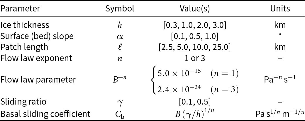
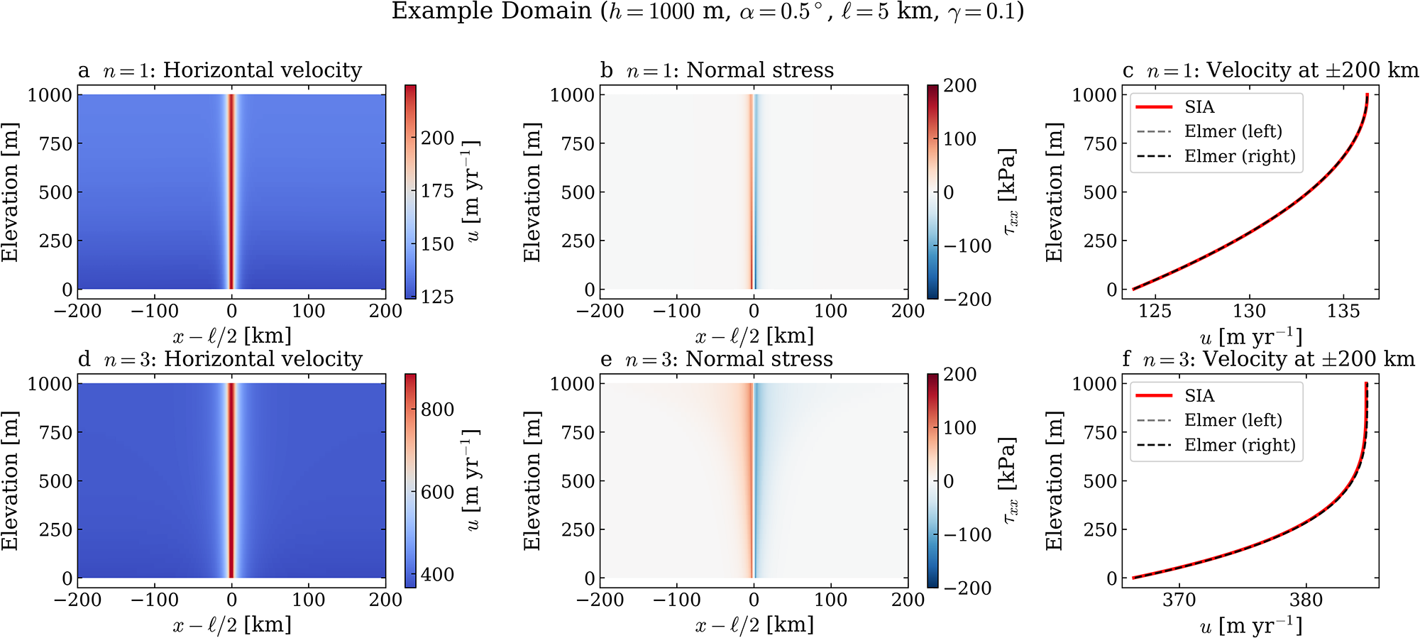


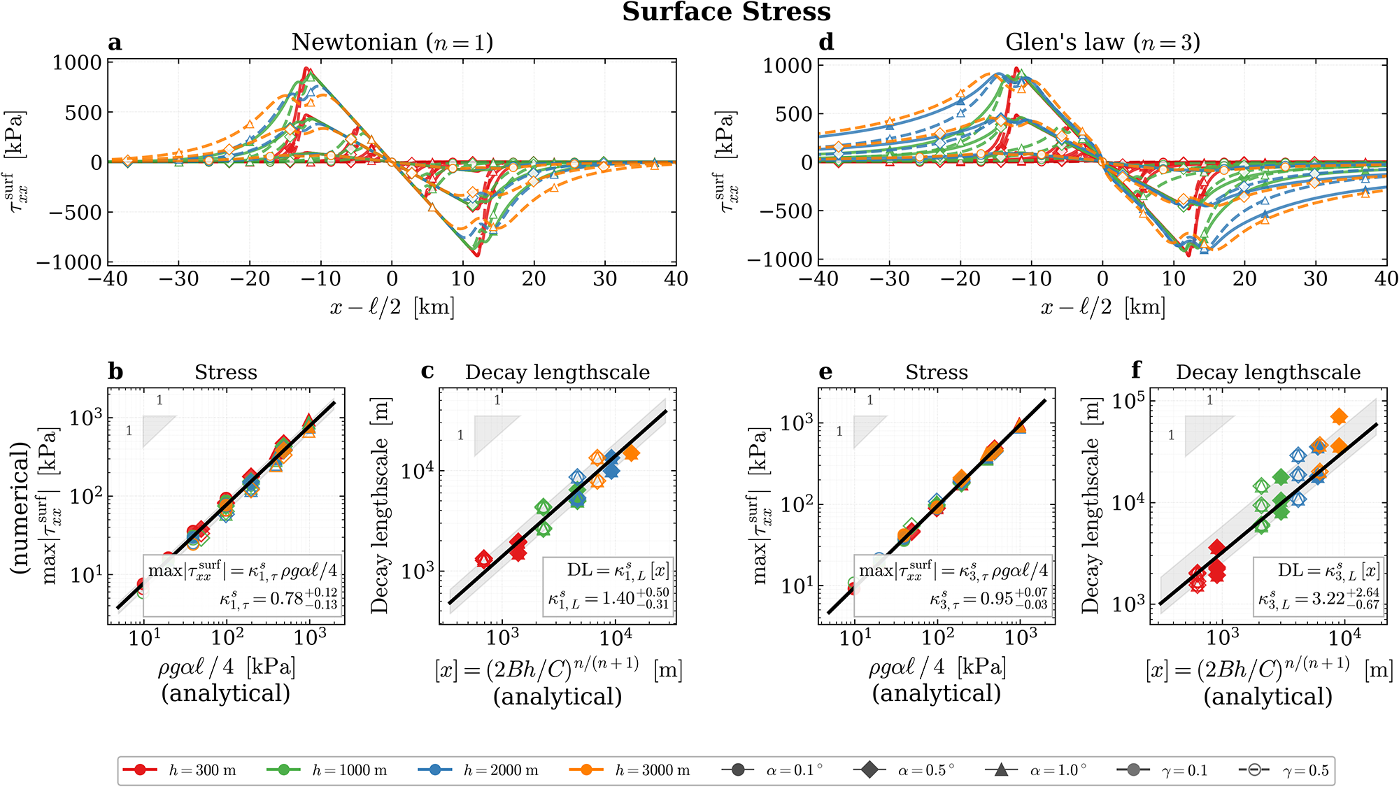


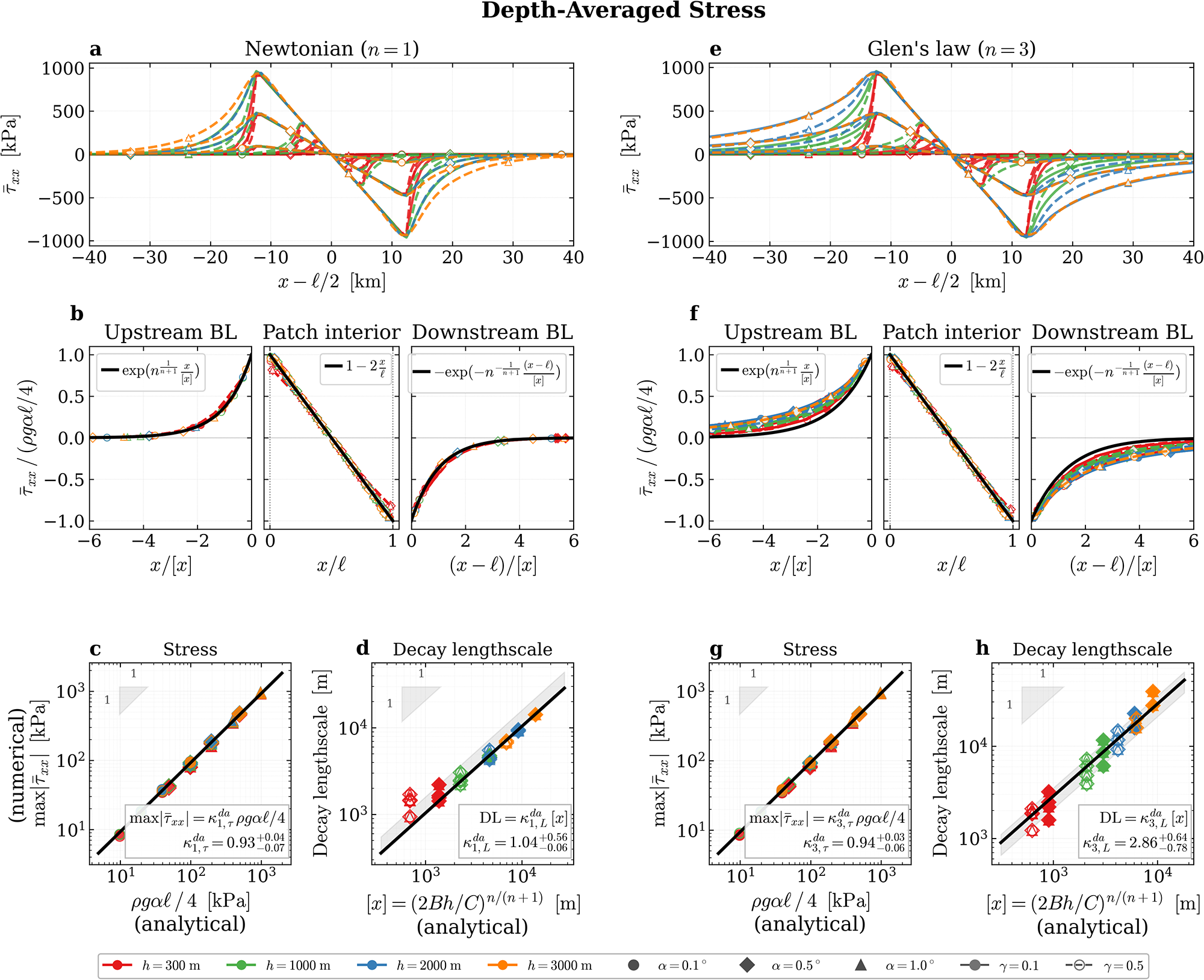


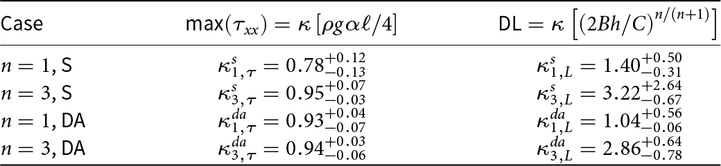


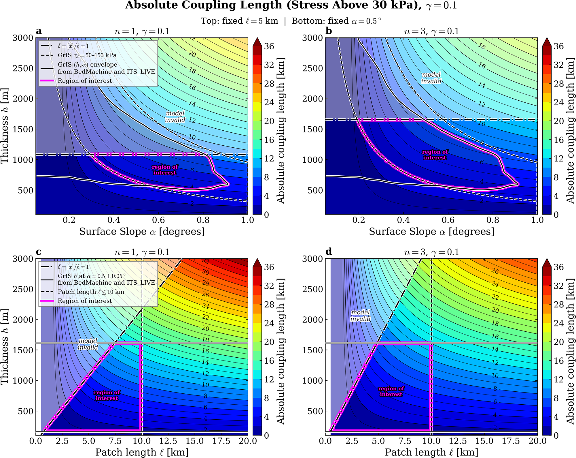


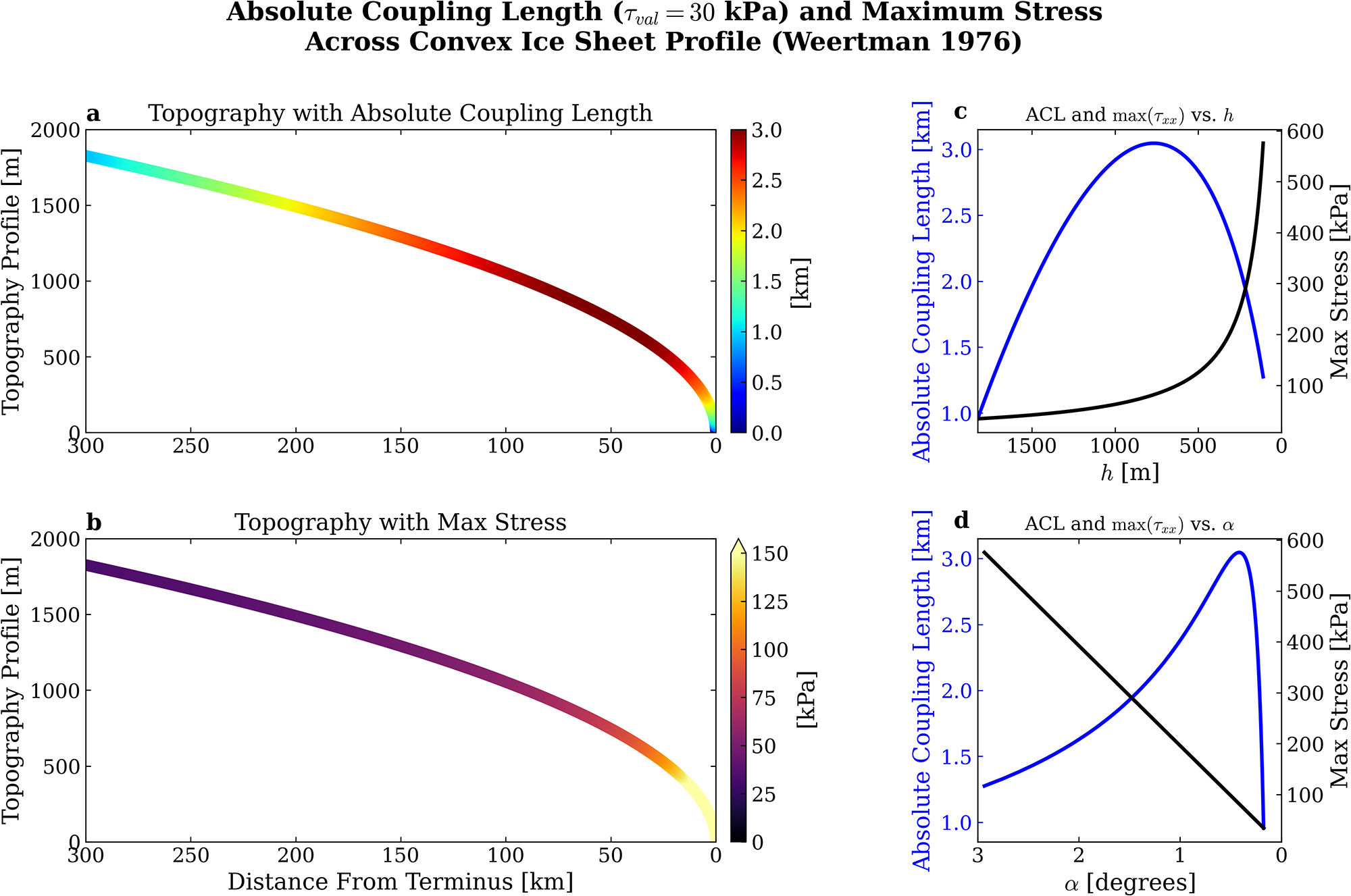


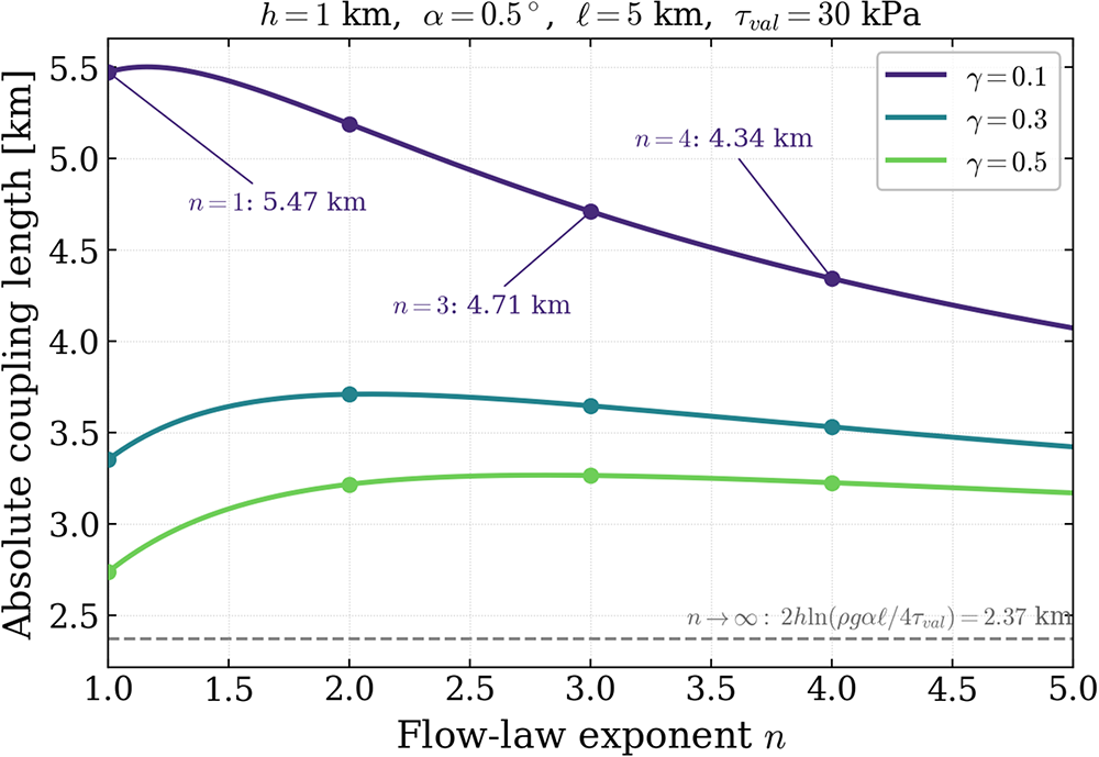


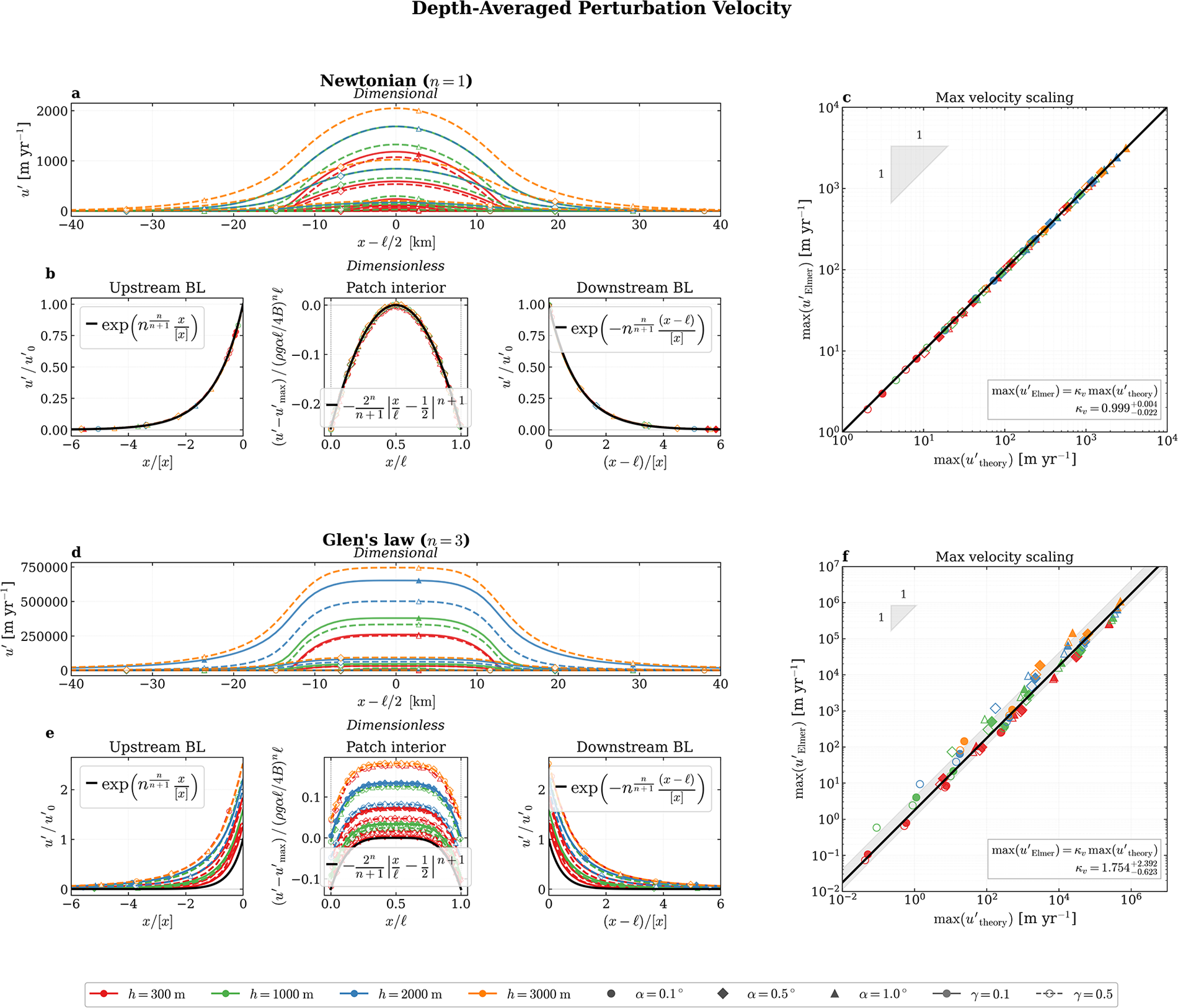


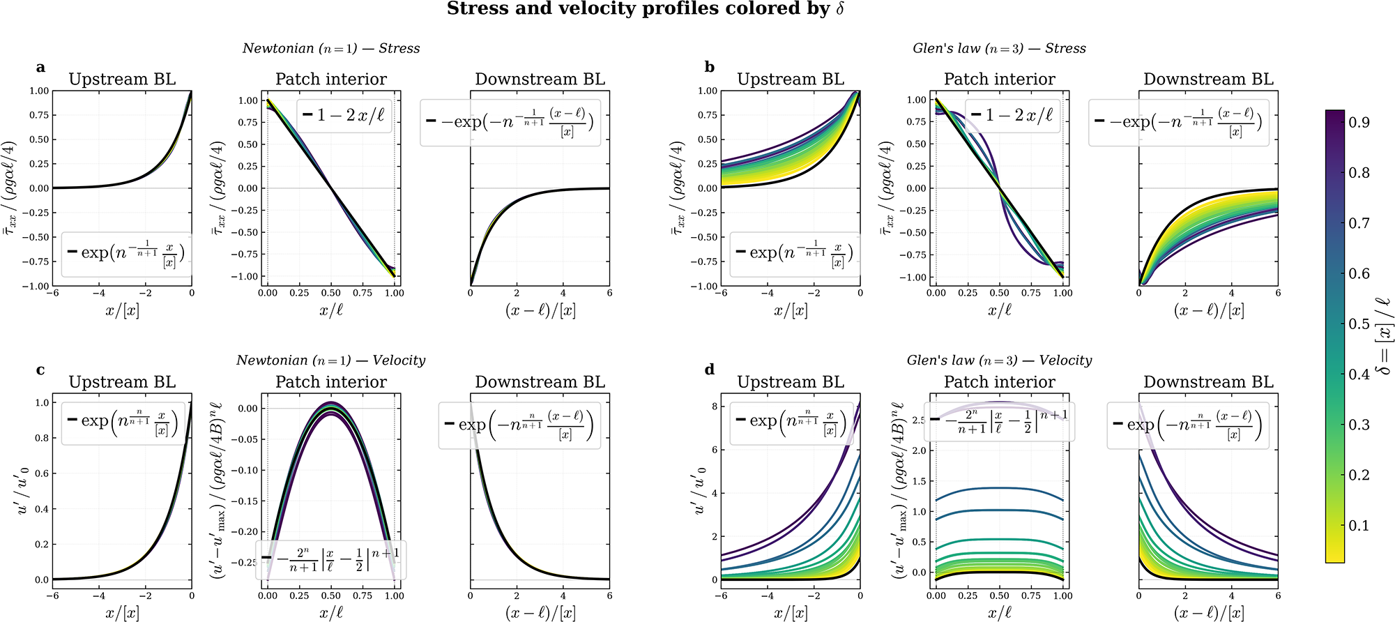


 Open access

