



1. Introduction
The stellarator as a fusion reactor concept is qualitatively different from the tokamak due to the inherently three-dimensional nature of the magnetic field. This added flexibility allows the stellarator approach to circumvent the need for toroidal plasma current to provide the confining poloidal magnetic field, meaning stellarators are less prone to potentially destructive plasma-current-driven instabilities (Gates et al. Reference Gates, Anderson, Anderson, Zarnstorf, Spong, Weitzner, Neilson, Ruzic, Andruczyk and Harris2018). One consequence of this improved magnetohydrodynamic (MHD) behaviour is the potential for robust high-$\beta$ operation, where $\beta = 8{\rm \pi} p / B_0^2$
 is the normalized plasma pressure, $p$
 is the electron pressure and $B_0$
 is the magnetic field strength, without the danger of current-driven instabilities. Even in the absence of large-scale MHD instability, the system may exhibit small-scale kinetic ballooning modes (KBMs), which could conceivably drive large energy and particle fluxes and thus be problematic for high-$\beta$
 operation of stellarators (Ishizawa et al. Reference Ishizawa, Maeyama, Watanabe, Sugama and Nakajima2013; Aleynikova & Zocco Reference Aleynikova and Zocco2017; Aleynikova et al. Reference Aleynikova, Zocco, Xanthopoulos, Helander and Nührenberg2018). The purpose of this work is to expand on previous analyses of KBM instability and turbulence by probing the properties of these modes in stellarator equilibria with low average magnetic shear $\hat {s} = - (r / \,\iota \!\!\!\!-) \,\textrm {d}\ \iota \!\!\!\!- / \textrm {d}r$
 , where $\,\iota \!\!\!\!-$
 is the rotational transform and $r$
 is a radial coordinate labelling flux surfaces. Low average magnetic shear $\hat {s}$
 is a notable design feature of some classes of neoclassical-transport-optimized stellarators such as the Helically Symmetric eXperiment (HSX). A deeper understanding of KBM saturation in such configurations will aid in the optimization of low-$\hat {s}$
 equilibria with respect to finite-$\beta$
 turbulent transport.
Neoclassical transport governs confinement in the classical stellarator. However, this issue can be quelled by ensuring that bounce-averaged particle excursions from a given flux surface during a banana orbit nearly vanish (Boozer Reference Boozer1983; Mynick Reference Mynick2006). There are a number of ways to reduce stellarator neoclassical transport to tokamak-like levels, such as quasi-symmetry (Nührenberg & Zille Reference Nührenberg and Zille1988; Rodríguez, Helander & Bhattacharjee Reference Rodríguez, Helander and Bhattacharjee2020) or quasi-isodynamicity (Palumbo Reference Palumbo1968; Mikhailov et al. Reference Mikhailov, Shafranov, Subbotin, Yu Isaev, Nührenberg, Zille and Cooper2002), both of which are subsets of quasi-omnigeneity (Hall & McNamara Reference Hall and McNamara1975; Yu Isaev et al. Reference Yu Isaev, Nührenberg, Mikhailov, Cooper, Watanabe, Yokoyama, Yamazaki, Subbotin and Shafranov2003). Magnetic configurations with sufficiently minimized neoclassical cross-field diffusion are dominated by anomalous transport (Canik et al. Reference Canik, Anderson, Anderson, Likin, Talmadge and Zhai2007; Hirsch et al. Reference Hirsch, Baldzuhn, Beidler, Brakel, Burhenn, Dinklage, Ehmler, Endler, Erckmann and Feng2008; Wolf et al. Reference Wolf, Alonso, Äkäslompolo, Baldzuhn, Beurskens, Beidler, Biedermann, Bosch, Bozhenkov and Brakel2019). Drift-wave turbulence is a primary candidate to explain anomalous transport in these configurations. Drift waves exist in a variety of types such as ion-temperature-gradient (ITG) modes (Rudakov & Sagdeev Reference Rudakov and Sagdeev1961; Horton, Choi & Tang Reference Horton, Choi and Tang1981; Xanthopoulos & Jenko Reference Xanthopoulos and Jenko2007; Mynick, Pomphrey & Xanthopoulos Reference Mynick, Pomphrey and Xanthopoulos2010; Xanthopoulos et al. Reference Xanthopoulos, Mynick, Helander, Turkin, Plunk, Jenko, Görler, Told, Bird and Proll2014; McKinney et al. Reference McKinney, Pueschel, Faber, Hegna, Talmadge, Anderson, Mynick and Xanthopoulos2019), trapped-electron modes (Coppi Reference Coppi1965; Coppi, Rosenbluth & Sadgeev Reference Coppi, Rosenbluth and Sadgeev1967; Kadomtsev & Pogutse Reference Kadomtsev and Pogutse1971; Faber et al. Reference Faber, Pueschel, Proll, Xanthopoulos, Terry, Hegna, Weir, Likin and Talmadge2015) or KBMs (Connor, Hastie & Taylor Reference Connor, Hastie and Taylor1978; Tang Reference Tang1978; Strauss Reference Strauss1979; Antonsen & Lane Reference Antonsen and Lane1980; Kotschenreuther Reference Kotschenreuther1986; Pueschel, Kammerer & Jenko Reference Pueschel, Kammerer and Jenko2008; Pueschel & Jenko Reference Pueschel and Jenko2010; Aleynikova et al. Reference Aleynikova, Zocco, Xanthopoulos, Helander and Nührenberg2018).
The KBMs are electromagnetic modes, as they require fluctuations in the magnetic field. Typically, the onset of KBM-driven turbulent transport is associated with breaching the ideal MHD ballooning stability boundary (Snyder Reference Snyder1999; Snyder et al. Reference Snyder, Hammett, Beer and Dorland1999; Pueschel et al. Reference Pueschel, Kammerer and Jenko2008; Pueschel & Jenko Reference Pueschel and Jenko2010). It has been shown that ion magnetic drifts can introduce an additional physical effect not present in simple MHD modelling in the small-perpendicular-wavelength limit (Kotschenreuther Reference Kotschenreuther1986; Aleynikova & Zocco Reference Aleynikova and Zocco2017). Specifically, coupling between a KBM and thermal ions provides additional free energy to the mode. This resonant effect arises from non-adiabatic contributions to the ion density fluctuations in a kinetic treatment of the governing equations (Hirose, Zhang & Elia Reference Hirose, Zhang and Elia1995; Hirose & Elia Reference Hirose and Elia1996). This effect can be qualitatively captured in a two-fluid treatment of the system, suggesting that the mode is of a reactive type since the kinetic treatment is unnecessary for qualitative purposes (Hirose & Elia Reference Hirose and Elia1996).
In the present work, the focus lies on the $\beta _{\rm crit}^{\rm KBM}$ value at which the KBM becomes the most unstable microinstability; for a discussion of different threshold definitions, see Pueschel et al. (Reference Pueschel, Kammerer and Jenko2008). An analysis of various Wendelstein 7-X equilibria (Aleynikova et al. Reference Aleynikova, Zocco, Xanthopoulos, Helander and Nührenberg2018), an optimized quasi-omnigenous stellarator, with respect to KBMs suggests both that, for sufficiently large $\beta$
 , peak KBM growth rates occur as $k_y \rightarrow 0$
 for a number of physically relevant parameter regimes and that the critical $\beta$
 at which KBMs become unstable is of the order of $\beta _{\rm crit}^{\rm KBM} \approx 1\,\%$
 , depending on the specific equilibrium. It is also shown in the same analysis that, in low-average-magnetic-shear Wendelstein 7-X configurations, KBMs can be destabilized before the ideal MHD limit $\beta _{\rm crit}^{\rm MHD}$
 . As will be shown here, this KBM threshold can be much lower than the MHD threshold $\beta _{\rm crit}^{\rm MHD}$
 , with $\beta _{\rm crit}^{\rm KBM} \approx 0.2\,\%$
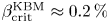 in the HSX (a quasi-helically symmetric stellarator) over a range of wavelengths, raising the possibility that such configurations exhibit poor KBM turbulence and confinement properties. However, it is shown here that the saturated nonlinear heat flux is greatly reduced relative to the electrostatic ITG case when $\beta > \beta _{\rm crit}^{\rm KBM}$
 . This implies that expectations based on linearly calculated $\beta _{\rm crit}^{\rm KBM}$
 values, e.g. that nonlinear heat fluxes tend to increase for $\beta > \beta _{\rm crit}^{\rm KBM}$
 , do not accurately account for critical nonlinear dynamics.
With the goal of developing a better understanding of the relationship between the magnetic geometry and $\beta _{\rm crit}^{\rm KBM}$ , the gyrokinetic turbulence code Gene is used here to perform electromagnetic nonlinear gyrokinetic local flux-tube simulations (Jenko Reference Jenko2000) (see http://www.genecode.org for code details and access). This paper is organized as follows. Section 2 introduces both the simulation framework for the present work and details regarding the three magnetic geometries. In § 3, linear and nonlinear electromagnetic simulations of KBMs and analyses thereof are presented. Section 4 shows the scaling of $\beta _{\rm crit}^{\rm KBM}$
 with the average magnetic shear and the normalized ITG and the similarities in linear KBM results between HSX, Heliotron-J and a circular tokamak. Lastly, conclusions are given in § 5.
2. Simulation approach and magnetic geometries
The gyrokinetic code Gene (Jenko Reference Jenko2000) is used in this work to investigate KBM and ITG turbulence via flux-tube simulations of low-average-magnetic-shear equilibria, namely HSX, the helical-axis Heliotron-J (H-J) (Obiki et al. Reference Obiki, Sano, Wakatani, Kondo, Mizuuchi, Hanatani, Nakamura, Nagasaki, Okada and Nakasuga2000) and a circular tokamak geometry. Gene solves a system of coupled equations that consists of the Vlasov equation, the Poisson equation and Ampère's law while taking advantage of the increased computational efficiency provided by gyro-averaging the orbits of charged particles in a strong magnetic guide field (Brizard & Hahm Reference Brizard and Hahm2007). For the full set of equations, see Pueschel et al. (Reference Pueschel, Jenko, Told and Buchner2011). Gene uses a five-dimensional phase space in which the coordinate system consists of the $x$ (radial), $y$
 (binormal), $z$
 (parallel to $\boldsymbol {B}_0$
 ), $v_\parallel$
 (parallel velocity space) and $\mu$
 (perpendicular velocity space) directions. There is both a box size $L$
 and a resolution $N$
 for each direction. For the nonlinear HSX calculation presented here, the resolutions, box sizes and hyperdiffusion coefficients are the following: $N_x = 128$
 , $N_y = 96$
 , $N_z = 512$
 , $N_{v\parallel } = 32$
 , $N_\mu = 8$
 , $L_y = 251.3 \rho _{s}$
 (corresponding to $k_y^{\rm min} \rho _{s} = 0.025$
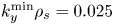 ), $L_x = 217.6 \rho _{s}$
 , $N_{\rm pol} = 4$
 , $D_z = 8$
 , and $D_{v\parallel } = 2$
 , where $\rho _{s} = c_{s} m_{i} / (eB)$
 is the ion sound gyroradius, $N_{\rm pol}$
 is the number of poloidal turns, $D_z$
 is the the parallel real-space hyperdiffusion coefficient and $D_{v\parallel }$
 is the parallel velocity-space hyperdiffusion coefficient (Pueschel, Dannert & Jenko Reference Pueschel, Dannert and Jenko2010). Numerical convergence studies were performed, including for $N_{\rm pol}$
 , to ensure that results presented here are numerically converged. Due to the significant extent along the field line of the KBMs studied in this work, $N_{\rm pol} = 4$
 is required to achieve convergence (Faber et al. Reference Faber, Pueschel, Terry, Hegna and Roman2018). If under-resolved in $N_{\rm pol}$
 , artificial reinforcement of the KBMs via the parallel boundary condition is possible, yielding unphysical results. This is consistent with previous work regarding trapped-electron modes in HSX and with recent studies of a tokamak geometry (Faber et al. Reference Faber, Pueschel, Terry, Hegna and Roman2018; Ball, Brunner & Ajay Reference Ball, Brunner and Ajay2020). Lastly, we do not include either parallel magnetic field fluctuations or collisions.
The MHD equilibrium solver VMEC (Hirshman, van Rij & Merkel Reference Hirshman, van Rij and Merkel1986) is used to generate the HSX and H-J equilibria, which are subsequently processed using the GIST code (Xanthopoulos et al. Reference Xanthopoulos, Cooper, Jenko, Turkin, Runov and Geiger2009). The coordinates are centred at the specified normalized toroidal magnetic flux $s_0 = \varPsi / \varPsi (a) = (r / a)^2$ , where $\varPsi (a)$
 is the toroidal flux at the plasma boundary and $a$
 is the effective minor radius. Details pertaining to the specifics of low-$\hat {s}$
 flux-tube geometries can be found in Faber et al. (Reference Faber, Pueschel, Terry, Hegna and Roman2018) and McKinney et al. (Reference McKinney, Pueschel, Faber, Hegna, Talmadge, Anderson, Mynick and Xanthopoulos2019) (HSX) and in Ishizawa et al. (Reference Ishizawa, Kishimoto, Watanabe, Sugama, Tanaka, Satake, Kobayashi, Nagasaki and Nakamura2017) (H-J). All three configurations have comparable values of the average magnetic shear $\hat {s}$
 along any given field line. As will be shown in this work, the average magnetic shear plays a critical role in determining $\beta _{\rm crit}^{\rm KBM}$
 , beyond the threshold prediction from MHD.
The magnetic equilibria used in this work are as follows. HSX is a four-field-period stellarator, where the number of field periods is defined as the number of times the magnetic geometry repeats per one toroidal transit, with aspect ratio $A = R_0 /a \approx 10$ , where $R_0$
 is the major radius, mean magnetic field $\langle B_0 \rangle \approx 1~{\rm T}$
 and low average magnetic shear $\hat {s} \approx - 0.05$
 at $s_0 = 0.5$
 . The major radius $R_0$
 (minor radius $a$
 ) of HSX is approximately $1.2\ {\rm m}$
 ($0.12\ {\rm m}$
 ). The HSX flux tube used throughout this work is centred at the outboard midplane, corresponding to $\alpha = 0$
 , where $\alpha = \theta - \,\iota \!\!\!\!- \zeta$
 is a field-line label and $\theta$
 and $\zeta$
 are the poloidal and toroidal angles in PEST coordinates, respectively, where PEST coordinates are a straight field-line coordinate system (Grimm, Greene & Johnson Reference Grimm, Greene and Johnson1976). It should also be noted that HSX is not optimized for a specific $\beta$
 , and therefore the HSX configuration used is given by the vacuum case with $\beta = 0$
 . This choice, however, is independent of the $\beta$
 used in $ {Gene}$
 . Investigation into the effect of including self-consistent, finite equilibrium $\beta$
 values was performed, and it was found that changing the equilibrium $\beta$
 does not significantly affect the results presented below. Figure 4, a plot of growth rate and real frequency spectra of HSX using both a $\beta = 0$
 equilibrium and a self-consistent $\beta = 0.48\,\%$
 equilibrium, highlights that there is no significant difference between the vacuum and finite-$\beta$
 cases. As a result, the $\boldsymbol {\nabla } B$
 and curvature $\kappa$
 drifts are taken to be the same in this work, as is consistent with a $\beta = 0$
 equilibrium. The H-J configuration used in this work has an equilibrium $\beta \approx 0.03\,\%$
 , four field periods, aspect ratio $A \approx 7.3$
 , mean magnetic field $\langle B_0 \rangle \approx 1.35\ {\rm T}$
 and average magnetic shear $\hat {s} \approx 0.028$
 , which is a factor of two smaller than that of HSX and of opposite sign, at $s_0 = 0.5$
 . The major radius $R_0$
 (minor radius $a$
 ) of H-J is $1.18\ {\rm m}$
 ($0.162\ {\rm m}$
 ). As was the case for HSX, the $\alpha = 0$
 flux tube is employed for H-J in this work. It should be reiterated that H-J is not a quasi-symmetric stellarator. Lastly, an $\hat {s}$
 –$\alpha$
 geometry, corresponding to a tokamak with circular flux surfaces, is used to investigate KBM dynamics in an axisymmetric system for comparison (Connor et al. Reference Connor, Hastie and Taylor1978). A value of average magnetic shear $\hat {s} = -0.052$
 is used throughout, as is a self-consistent (with $\beta$
 and the pressure gradients) $\alpha _{\rm MHD} = \,\iota \!\!\!\!-^{-2} (R_0 / L_n) [\beta _{e}(1 + \eta _{e}) + \beta _{i} (1 + \eta _{i})]$
 , where $L_n$
 and $\eta _{({i},{e})}$
 are the density gradient scale length and the ratio of the (ion, electron) temperature gradient to the density gradient, respectively. It should be noted that since a negative value of $\hat {s}$
 is used, this tokamak equilibrium is stable to ideal MHD ballooning, $\beta _{\rm crit}^{\rm MHD} \to \infty$
 (Greene & Chance Reference Greene and Chance1981; Antonsen et al. Reference Antonsen, Drake, Guzdar, Hassam, Lau, Liu and Novakovskii1996).
3. Electromagnetic ITG and KBM turbulence
3.1. Linear eigenmodes in low-$\hat {s}$ configurations

Typically, as $\beta$ increases, the normalized ITG growth rates $\gamma$
 in units of $c_{s} / a$
 , where $c_{s}$
 is the sound speed, steadily decrease (Pu & Migliuolo Reference Pu and Migliuolo1985; Dong, Guzdar & Lee Reference Dong, Guzdar and Lee1987; Kim, Horton & Dong Reference Kim, Horton and Dong1993). This is known as finite-$\beta$
 ITG stabilization, or linear electromagnetic stabilization. The mechanism by which this stabilization occurs is the coupling between the ITG mode and the shear Alfvén wave. This efficiently transfers energy out of the ITG mode, reducing its growth. Alterations of the ion Landau resonance due to finite-equilibrium-$\beta$
 $\boldsymbol {\nabla } B$
 modifications from the bending of perturbed field lines can also play a role in the stabilization (Jarmén, Anderson & Malinov Reference Jarmén, Anderson and Malinov2015). This reduction in growth rate will tend to reduce the nonlinear heat flux, but additional physics can also have an impact on the dynamics.
Another mechanism that affects ITG transport levels as $\beta$ increases is nonlinear electromagnetic stabilization (Pueschel et al. Reference Pueschel, Kammerer and Jenko2008; Pueschel & Jenko Reference Pueschel and Jenko2010; Whelan, Pueschel & Terry Reference Whelan, Pueschel and Terry2018; Whelan et al. Reference Whelan, Pueschel, Terry, Citrin, McKinney, Guttenfelder and Doerk2019). As $\beta$
 increases, one observes a reduction in nonlinear heat flux that is greater than the reduction in linear growth rates or quasilinear fluxes. As has been shown in Whelan et al. (Reference Whelan, Pueschel and Terry2018, Reference Whelan, Pueschel, Terry, Citrin, McKinney, Guttenfelder and Doerk2019), the difference between the (quasi-)linear and nonlinear reduction stems from changes in the efficiency of zonal-flow-mediated energy transfer to stable modes. This effect has been shown to be active in a range of configurations, both of tokamak and of stellarator type. It has also been demonstrated that the inclusion of a self-consistent Shafranov shift can eliminate nonlinear electromagnetic stabilization for different, specific parameter regimes (Ishizawa et al. Reference Ishizawa, Urano, Nakamura, Maeyama and Watanabe2019).
The physical mechanism underlying KBM destabilization is the following. As with most microinstabilities, KBMs are destabilized when the driving force associated with the pressure gradient is sufficiently strong in the bad curvature region to overcome the stabilizing force from the magnetic field (Cheng Reference Cheng1982). More specific to KBMs, the modifications to magnetic drifts by $\beta$ -induced magnetic fluctuations result in destabilizing effects when a kinetic treatment is applied to the governing equations. This is due to a resonance between the KBM and thermal ions, giving the KBM an additional free energy source.
For the cases studied here, the dominant eigenmode for $\beta < \beta _{\rm crit}^{\rm KBM}$ is ITG, whose growth rate decreases with $\beta$
 . For $\beta \geq \beta _{\rm crit}^{\rm KBM}$
 , KBM has a larger growth rate than the ITG mode with the growth rate increasing rapidly with $\beta$
 . This critical value $\beta _{\rm crit}^{\rm KBM}$
 is generally of the order of 1 % in standard tokamaks and is comparable to the ideal MHD ballooning $\beta$
 limit for physically relevant gradient values (see Pueschel et al. Reference Pueschel, Kammerer and Jenko2008; Pueschel & Jenko Reference Pueschel and Jenko2010; Ishizawa et al. Reference Ishizawa, Maeyama, Watanabe, Sugama and Nakajima2013). However, $\beta _{\rm crit}^{\rm KBM}$
 is not always close to $\beta _{\rm crit}^{\rm MHD}$
 and is, in general, a complicated function of the magnetic geometry.
Before presenting analyses of nonlinear simulations, the behaviour and scaling of linear instability will be elucidated, for both dominant and subdominant eigenmodes. Typically, ITG and KBM growth rates decrease and increase, respectively, as $\beta$ increases. Figure 1 highlights this behaviour in HSX at normalized binormal wavenumber $k_y \rho _{s} = 0.6$
 . Henceforth, normalized wavenumbers are denoted $k_y \rho _{s} \rightarrow k_y$
 . The normalized gradients, $\beta$
 and the temperature ratio used in these calculations and throughout this work are $a / L_{T{i}} = 3$
 and $a / L_{T{e}} = a / L_n = 1$
 , $\beta = 0.48\,\%$
 and $T_{i} / T_{e} = 1$
 , respectively, unless otherwise stated. Note the factor-of-three reduction in the ITG growth rate as $\beta$
 increases before the KBM becomes dominant. This significant reduction in ITG growth rate is not observed for all values of $k_y$
 , as evidenced by figure 2, where at $k_y = 0.1$
 there is no significant reduction in $\gamma$
 before KBMs become dominant for either the $N_{\rm pol} = 1$
 or the $N_{\rm pol} = 4$
 case. This is partially due to the fact that, in the $k_y = 0.1$
 case, the KBM becomes dominant at a small critical normalized plasma pressure $\beta _{\rm crit}^{\rm KBM} \approx 0.18\,\%$
 versus $\beta _{\rm crit}^{\rm KBM} \approx 2.2\,\%$
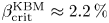 for the $k_y = 0.6$
 case. Also note that $N_{\rm pol} = 4$
 is required to achieve convergence, as elongated eigenmodes can artificially self-reinforce via the parallel boundary condition.
The growth rate and real frequency for the eigenmode with the largest growth rate at $k_y = 0.6$ over a range of $\beta$
 values for HSX with $a / L_{T{i}} = 3$
 and $a / L_{T{e}} = a / L_n = T_{i} / T_{e} = 1$
 . Note the stabilization of ITG growth rates (shown as triangles) as $\beta$
 increases and approaches $\beta _{\rm crit}^{\rm KBM} \approx 2.2\,\%$
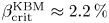 , where there is a clear discontinuity in real frequency, which highlights the change in dominant mode branch from ITG to KBM (shown as diamonds).

Growth rate and real frequency for $k_y = 0.1$ of the HSX configuration with $a / L_{T{i}} = 3$
 and $a / L_{T{e}} = a / L_n = T_{i} / T_{e} = 1$
 for both $N_{\rm pol} = 1$
 (blue diamonds) and $N_{\rm pol} = 4$
 (black triangles). Note the lack of ITG stabilization relative to the $k_y = 0.6$
 case and the significant difference between the two cases, an indication that $N_{\rm pol} = 1$
 is insufficient for convergence. Also, $\beta _{\rm crit}^{\rm KBM}$
 is much lower for this case.

The scaling of $\beta _{\rm crit}^{\rm KBM}$ with $k_y$
 is presented in figure 3 for both HSX (blue squares) and NCSX (black triangles), a quasi-axisymmetric stellarator configuration optimized for operation at $\beta \approx 4.2\,\%$
 (Neilson, Zarnstorff & Lyon Reference Neilson, Zarnstorff and Lyon2002) with $\hat {s} \approx -0.5$
 at $s_0 = 0.5$
 . For HSX, $\beta _{\rm crit}^{\rm KBM}$
 is small relative to the ideal MHD ballooning limit $\beta _{\rm crit}^{\rm MHD}$
 , and considerably smaller than the high-$\hat {s}$
 NCSX analogue where $\beta _{\rm crit}^{\rm KBM}$
 is comparable to $\beta _{\rm crit}^{\rm MHD}$
 . The normalized gradients and temperature ratio used in the NCSX calculations are the same as were used for HSX. The ideal ballooning limit $\beta _{\rm crit}^{\rm MHD}$
 is also shown as a horizontal dashed line for each configuration. The NCSX curve smoothly approaches the MHD limit as $k_y$
 decreases until $k_y < 0.1$
 where there is a slight uptick in $\beta _{\rm crit}^{\rm KBM}$
 . The HSX curve is well below the MHD limit in the transport-relevant $k_y < 0.25$
 range, and dips to values $\approx 0.1\,\%$
 that are an order of magnitude smaller than $\beta _{\rm crit}^{\rm MHD}$
 . This suggests that conditions in HSX are more conducive to KBM excitation due to ion kinetic physics (see § 4) than they are in NCSX. As will be shown, this is associated with the low average magnetic shear in HSX.
The $\beta _{\rm crit}^{\rm KBM}$ spectrum of NCSX (black triangles) and HSX (blue squares) with $a / L_{T{i}} = 3$
 and $a / L_{T{e}} = a / L_n = T_{i} / T_{e} = 1$
 . Horizontal dashed lines correspond to $\beta _{\rm crit}^{\rm MHD}$
 . Note the low $\beta _{\rm crit}^{\rm KBM}$
 relative to $\beta _{\rm crit}^{\rm MHD}$
 for HSX compared to NCSX.

Figure 4 shows the dominant growth rates $\gamma$ and real frequencies $\omega$
 as functions of $k_y$
 at a constant $\beta = 0.48\,\%$
 . It is worth noting that KBM is dominant over a certain range of $k_y$
 values, namely $k_y \in [0.1,0.2]$
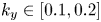 , while ITG is dominant over the remainder of the wavelength range. This means that nonlinear calculations of HSX at this value of $\beta$
 will potentially exhibit concurrent ITG and KBM drive characteristics, a phenomenon that is also observed in nonlinear simulations of tokamaks if $\beta \geq \beta _{\rm crit}^{\rm KBM}$
 (Pueschel et al. Reference Pueschel, Kammerer and Jenko2008; Pueschel & Jenko Reference Pueschel and Jenko2010).
Growth rate and real frequency spectra for the HSX configuration (both with an equilibrium $\beta = 0$ (black) and equilibrium $\beta = 0.48\,\%$
 (blue)) with $a / L_{T{i}} = 3$
 , $\beta = 0.48\,\%$
 and $a / L_{T{e}} = a / L_n = T_{i} / T_{e} = 1$
 . The KBMs (ITG modes) are denoted by diamonds (triangles). Note the transition from ITG to KBM (at roughly $k_y \approx 0.1$
 ) and back to ITG (at roughly $k_y \approx 0.2$
 ), highlighted by the discontinuity in real frequency. Also note the similarity in the two spectra when using a finite-$\beta$
 magnetic equilibrium versus using the vacuum case.

Lastly, the subdominant mode spectrum of HSX at $k_y = 0.2$ with $\beta = 0.5\,\%$
 , shown in figure 5, indicates that there is not just a single KBM that is destabilized as $\beta$
 increases, but rather there are two families of KBMs, one of which is a set of modes that are centred at the outboard midplane ($\theta _p=0$
 ) and another that consists of pairs of sibling modes that peak away from the outboard midplane ($\theta _p \neq 0$
 ). It should be noted that some of the centred KBMs exhibit tearing parity (blue and green curves in figure 5b), i.e. the $\varPhi$
 eigenfunctions are odd in ballooning angle. The low background magnetic shear in the present scenario enables destabilization of these modes, termed tearing-parity KBMs, which had previously been conjectured not to exist based on a study involving high-shear equilibria (Pueschel et al. Reference Pueschel, Hatch, Ernst, Guttenfelder, Terry, Citrin and Connor2019). It is worth noting that it is unlikely that the tearing-parity KBMs discussed here are micro tearing modes because of the unique ITG dependence of the modes, the fact that the modes propagate in the ion diamagnetic direction and the relatively small electron thermal transport nonlinearly, three qualities that are not characteristic of micro tearing modes. For each mode that peaks away from the outboard midplane, a sibling mode exists with the same growth rate and frequency with an eigenmode structure that is near-perfectly mirrored with respect to $\theta _p = 0$
 . The physics implication of this is that HSX is qualitatively different from typical high-$\hat {s}$
 tokamak cases, where only a single KBM is destabilized. Eigenvalue calculations with different gradients, $a / L_{T{i}} = 4$
 for example (with $a / L_n$
 and $a / L_{T{e}}$
 kept fixed), also exhibit the two branches of KBMs. However, the exact location of minimal $\beta _{\rm crit}^{\rm KBM}$
 shifts in $k_y$
 space relative to the $a / L_{T{i}} = 3$
 case. The region of $k_y$
 space in which the outboard-midplane-peaked KBMs are dominant shifts to smaller $k_y$
 as $\omega _{T{i}}$
 increases. It should also be noted that the two branches of KBMs are robustly present when ensuring numerical convergence. This also complicates analysis of the nonlinear energy dynamics, as there may be a number of unstable KBMs involved in nonlinear energy transfer.
The subdominant spectrum (a) for HSX with $k_y = 0.2$ and $\beta = 0.5\,\%$
 consisting of KBMs (diamonds) and ITG modes (triangles), and the associated electrostatic potential $\varPhi$
 eigenmode structures (b) for various KBMs. Note the two distinct families of KBMs: one with $\varPhi$
 symmetric about $\theta _p = 0$
 and one with off-centre peaking. For each mode of the latter family, there is a sibling mode that is mirrored across the $\theta _p = 0$
 axis with identical $\gamma$
 and $\omega$
 ; hence they are indistinguishable in (a). Also note that some of the centred KBMs (blue, green) have tearing parity, i.e. are odd functions of ballooning angle.

3.2. Nonlinear characteristics of the ITG–KBM system
Previous studies of KBM instability and turbulence have found critical $\beta$ values of the order of one or a few per cent for experimentally relevant gradient values and magnetic geometries (Pueschel et al. Reference Pueschel, Kammerer and Jenko2008; Pueschel & Jenko Reference Pueschel and Jenko2010; Ishizawa et al. Reference Ishizawa, Maeyama, Watanabe, Sugama and Nakajima2013). These analyses also show that for $\beta < \beta _{\rm crit}^{\rm KBM}$
 , the resulting turbulence is solely ITG or trapped-electron mode and for $\beta > \beta _{\rm crit}^{\rm KBM}$
 , signatures of multiple modes are present and observable in the simulations concurrently. Contrary to these cases, when $\beta > \beta _{\rm crit}^{\rm KBM}$
 , nonlinear simulations of the present HSX case do not achieve saturation when the minimum binormal wavenumber $k_y^{\rm min}$
 of the system is unstable to KBMs. In such simulations, streamer modes span the length of the periodic radial domain, regardless of how large the radial box is, and self-reinforce via the radial periodic boundary condition of the flux tube. However, if one chooses $k_y^{\rm min}$
 so that it is stable to KBMs, saturation can be achieved in electromagnetic flux-tube simulations, where a significant reduction in transport is observed relative to the near-electrostatic ($\beta = 0.05\,\%$
 ) case. The time traces of heat flux (both ion electrostatic and electron electromagnetic) and particle flux for $k_y^{\rm min} = 0.025$
 are shown in figure 6. Despite the KBM being an electromagnetic mode, below the threshold it does not drive significant electromagnetic flutter heat transport given the choice of small electron temperature gradient $a / L_{T{e}} = 1$
 . While the condition that the smallest finite $k_y$
 must be KBM-stable is empirical, one possible underlying cause is the ability of the system to terminate an inverse cascade by means of ITG (stable) eigenmodes. The precise nature of the phenomenon is left for future study.
Heat (both ion electrostatic (black) and electron electromagnetic (blue)) and particle flux (red) time traces for HSX with $k_y^{\rm min} = 0.025$ and $\beta = 0.48\,\%$
 . There is a significant (factor of $\approx 5$
 ) reduction in $Q_{i}^{\rm es}$
 relative to the near-electrostatic ($\beta \approx 0.05\,\%$
 ) case (McKinney et al. Reference McKinney, Pueschel, Faber, Hegna, Talmadge, Anderson, Mynick and Xanthopoulos2019). There is negligible, slightly negative magnetic flutter transport, a result of the low electron temperature gradient $a / L_{T{e}} = 1$
 .

The heat flux spectrum given in figure 7 shows that the ion electrostatic heat flux $Q_{i}^{\rm es}(k_y)$ peaks in the $k_y$
 range that is dominated by KBMs, consistent with the fact that $\beta$
 is roughly three times as large as $\beta _{\rm crit}^{\rm KBM}$
 for $k_y = 0.1$
 . Figure 7 also shows that KBM transport is the dominant physics mechanism nonlinearly as long as KBMs are destabilized linearly, even if KBM growth rates are subdominant, where linear destabilization is shown in figure 4. As discussed above, $k_y^{\rm min}$
 is sufficiently small that no KBM instability occurs at that mode; this is consistent with findings in high-$\hat {s}$
 scenarios where nonlinear saturation is possible for $\beta$
 values up to $\beta _{\rm crit}^{\rm KBM}$
 as $k_y \rightarrow 0$
 (Pueschel & Jenko Reference Pueschel and Jenko2010). The nonlinear electrostatic potential $\varPhi$
 spectrum is depicted in figure 8, showing that the simulation is not dominated by a zonal flow, as the $k_y=0.1$
 non-zonal component of $\varPhi$
 is a factor of nearly two larger than the zonal component and the sum of the non-zonal contributions is significantly larger than the zonal contribution. This is an indication that zonal flows may play at most a minor role in saturation. This view is refined, however, based on nonlinear energy transfer analysis.
Heat flux spectra for HSX with $k_y^{\rm min} = 0.025$ and $\beta = 0.48\,\%$
 (black) associated with the time trace shown in figure 6 and with $k_y^{\rm min} = 0.025$
 and $\beta = 0.24\,\%$
 (blue) for comparison. Note that the peaks of the spectra are almost fully contained in the binormal wavelength range over which KBM is destabilized, which is denoted by the shaded region. This shows that KBM transport dominates nonlinearly when KBMs are linearly destabilized, even if KBM growth rates are subdominant to ITG growth rates.

The nonlinear $\varPhi$ spectrum for HSX with $k_y^{\rm min} = 0.025$
 and $\beta = 0.48\,\%$
 . The spectrum is truncated at $k_y \rho _{s} = 0.5$
 since $|\varPhi |^2$
 amplitudes are negligible above this threshold. Note that the zonal component is much weaker than the integrated non-zonal amplitudes.

Nonlinear frequencies are shown in figure 9. Interestingly, there is no discontinuity in the nonlinear frequency spectrum of the HSX configuration, a feature that was present linearly at the ITG–KBM transition points in figure 4. Both dominant and subdominant linear KBM frequencies are overlaid in figure 9 to facilitate comparison with the nonlinear data. Clearly, throughout the range where linear data are shown, nonlinear frequency signatures match the values associated with the dominant outboard-centred KBMs. An exact frequency match is not expected to occur, as turbulence may result in a $k_y$ -dependent nonlinear frequency shift and broadening. This constitutes evidence that KBMs do indeed play an important role in the nonlinear turbulent state.
The nonlinear frequency spectrum for HSX with $k_y^{\rm min} = 0.025$ and $\beta = 0.48\,\%$
 . The colour scale has arbitrary units and is linear and normalized at each $k_y$
 separately. Linear frequencies of the most unstable (gold crosses), maximal-frequency (green triangles), minimal-frequency (red squares) and most unstable outboard-centred (black–white dashed diamonds) KBMs are also included for comparison. Note the agreement between the dominant linear outboard-centred KBM frequencies and the nonlinear signal.

Analysis of the nonlinear energy transfer to a given ($k_x$ ,$k_y$
 ) point in Fourier space due to interaction with ($k^\prime _x$
 ,$k^\prime _y$
 ) and ($k_x-k^\prime _x,k_y-k^\prime _y$
 ) also suggests that modes in the KBM-dominated $k_y$
 range play an important role in the energy transfer dynamics of the turbulence and therefore in the dynamics that leads to saturation. Figure 10 shows nonlinear energy transfer at a given ($k_x=0.06$
 , $k_y=0.1$
 ), denoted by the tip of the black arrow, to and from various ($k^\prime _x$
 , $k^\prime _y$
 ). Regions of blue correspond to locations which cause energy input into ($k_x=0.06$
 , $k_y=0.1$
 ) while red regions correspond to locations which draw energy from ($k_x=0.06$
 , $k_y=0.1$
 ). The dominant method by which ($k_x=0.06$
 , $k_y=0.1$
 ) receives energy is zonal energy transfer, indicated by the blue clouds at both $k^\prime _y=0$
 and $k^\prime _y = 0.1$
 . There is also significant non-zonal energy transfer via ($k^\prime _x=0.12$
 , $k^\prime _y=-0.025$
 ). It is important to note both that the largest energy sinks are due to non-zonal transfer and that the largest energy sinks are even larger than the largest energy inputs from zonal transfer. Lastly, the zonal energy transfer can occur due to both the zonal flow and the zonal field, i.e. the zonal component of the fluctuating magnetic field.
Nonlinear energy transfer functions indicate locations which give (blue) and receive (red) energy to and from ($k_x = 0.06$ , $k_y = 0.1$
 ), denoted by the tip of the black arrow. There is significant zonal transfer from ($k_x = 0.06$
 , $k_y = 0.1$
 ) to the blue clouds near $k^\prime _y=0$
 and $k^\prime _y = 0.1$
 . Significant non-zonal energy transfer is also observed at $k^\prime _y = -0.025$
 and $k^\prime _y = 0.125$
 .

This result appears to contradict the earlier finding in figure 8 that the zonal-flow amplitudes are low. However, when coupling is sufficiently resonant, zonal flows can very efficiently mediate energy transfer even if they are only excited to low amplitudes.
Further analysis of nonlinear energy transfer yields insight into the wavelength ranges which dominate energy transfer between the turbulence and the zonal ($k_y=0$ ) modes. Figure 11 shows normalized nonlinear energy transfer corresponding to $k_y=0$
 modes summed over both $k_x$
 and $k^\prime _x$
 versus $k^\prime _y$
 . The peak of the data occurs at $k^\prime _y = 0.125$
 , well within the KBM-dominated $k_y$
 range. A significant portion of the energy transfer to and from zonal modes is facilitated by modes in the KBM-dominated $k_y$
 range, constituting additional evidence that KBMs are important nonlinearly. One can also construct a quantity to gauge the relative importance of a given $k_y$
 in the overall nonlinear energy transfer dynamics, as highlighted by figure 12, a plot of averaged nonlinear energy transfer functions versus $k_y$
 . This quantity is the sum (over $k_x \neq 0$
 ) of the root mean squares (of each $k^\prime _x$
 –$k^\prime _y$
 plane) of the nonlinear energy transfer functions corresponding to a given ($k_x$
 ,$k_y$
 ). Both the zonal modes and KBMs contribute to the overall nonlinear energy transfer dynamics, with KBMs contributing roughly twice as much if one integrates over the entire KBM-dominated $k_y$
 range.
The sum (over $k_x \neq 0$ ) of the root mean squares (over coupled $k_x^\prime$
 ) of time-averaged nonlinear energy transfer functions for zonal ($k_y = 0$
 ) modes as a function of $k^\prime _y$
 . The data are normalized to the value of the point at $k^\prime _y = 0.125$
 . Note that the peak is in the KBM-dominated $k^\prime _y$
 range, evidence that KBMs play an important role in zonal dynamics.

The sum (over $k_x \neq 0$ ) of the root mean squares (over coupled $k_x^\prime$
 , $k_y^\prime$
 ) of time-averaged nonlinear energy transfer functions, which are normalized by the value of the same quantity at $k_y = 0.1$
 .

Lastly, figure 13 shows both the electrostatic ion heat and particle fluxes as $\beta$ increases. Simulations with $k_y^{\rm min} = 0.025$
 for $\beta = 0.75\,\%$
 and $1\,\%$
 grow without bounds and therefore do not have associated data points. This is consistent with the requirement that $k_y^{\rm min}$
 be stable to KBMs for saturation to occur, as $\beta _{\rm crit}^{\rm KBM} \approx 0.6\,\%$
 for $k_y = 0.025$
 , as shown in figure 3. Note the decrease in heat flux as $\beta$
 increases until $\beta$
 is sufficiently close to $\beta _{\rm crit}^{\rm KBM}(k_y^{\rm min})$
 , a result that is consistent with ITG nonlinear finite-$\beta$
 stabilization. The uptick in $Q_{i}^{\rm es}$
 as $\beta$
 increases from $0.48\,\%$
 to $0.55\,\%$
 is an expression of the KBMs, which, unlike the ITG modes, become more virulent as $\beta$
 is increased.
Normalized ion heat flux $Q_{i}^{\rm es}$ (black diamonds) and particle flux $\varGamma ^{\rm es}$
 (red squares) as a function of $\beta$
 . Observe the significant reduction of transport for $\beta \gtrsim 0.2\,\%$
 relative to $\beta \approx 0.05\,\%$
 until $\beta$
 approaches the $\beta _{\rm crit}^{\rm KBM} \approx 0.6\,\%$
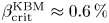 threshold for $k_y = 0.025$
 . Above $\beta = 0.6\,\%$
 , simulations no longer achieve a saturated state. The vertical dashed black line indicates $\beta _{\rm crit}^{\rm KBM}=0.6\,\%$
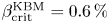 at $k_y = 0.025$
 and the vertical dotted black line indicates $\beta _{\rm crit}^{\rm KBM} = 0.18\,\%$
 at $k_y = 0.1$
 . The electron electromagnetic heat flux is negligible (normalized $Q_{e}^{\rm em} \approx -0.2$
 for $\beta = 0.48\,\%$
 ) and therefore not included in this analysis.

4. Impact of average magnetic shear and ITG
Further investigation demonstrates that $\hat {s}$ and $a / L_{T{i}}$
 are particularly important in setting the value of $\beta _{\rm crit}^{\rm KBM}$
 relative to the ideal ballooning threshold. This section addresses how the linear KBM characteristics presented in § 3 change as both the average magnetic shear $\hat {s}$
 and the fractional component of the total pressure gradient $a / L_{p}$
 driven by the ITG $a / L_{T{i}}$
 change. Linear results pertaining to H-J and a circular geometry with low $\hat {s}$
 are also shown.
Figure 14 presents $\beta _{\rm crit}^{\rm KBM}$ as a function of $\hat {s}$
 and demonstrates that the KBM threshold increases with $|\hat {s}|$
 , regardless of sign. This is consistent with the observations that, in general, drift waves are commonly stabilized by increased $|\hat {s}|$
 (Pearlstein & Berk Reference Pearlstein and Berk1969; Ross & Mahajan Reference Ross and Mahajan1978). Modification of the average magnetic shear of the flux tube is done self-consistently in the sense that the derivative of $\,\iota \!\!-$
 is adjusted to yield the desired $\hat {s}$
 and then geometric elements are recalculated accordingly. Furthermore, eigenvalue calculations of HSX with artificially high $\hat {s}$
 yield a subdominant mode spectrum that corresponds to the usual tokamak, single-unstable-KBM scenario, as well as to the NCSX configuration discussed in § 3.1. The physics implication of this result is that with increased shear, modes are less extended along the magnetic field line and therefore cannot access free energy in gradients via the bad curvature regions further along the field line, as evidenced by figure 15, a plot of two characteristic $\varPhi$
 eigenmodes for the $\hat {s}=-0.05$
 case (black) and the $\hat {s} = 0.5$
 case (blue). Conversely, KBMs are therefore more easily destabilized with more free energy to access when $|\hat {s}|$
 is low like in HSX.
The $\beta _{\rm crit}^{\rm KBM}$ as a function of $\hat {s}$
 for the HSX configuration with $k_y = 0.1$
 . The vertical dashed red line highlights the self-consistent nominal $\hat {s}$
 for HSX at $s_0 = 0.5$
 . Note that $\beta _{\rm crit}^{\rm KBM}$
 increases as the magnitude of the average magnetic shear increases, regardless of sign.

Characteristic $\varPhi$ eigenmode structures for KBMs for the HSX geometries with $\hat {s} = -0.05$
 (black) and $\hat {s} = 0.5$
 (blue) which highlight the extended nature of the eigenmodes when the magnitude of the average magnetic shear is low. The mode structure magnitudes are normalized to their values at the outboard midplane.

This result is consistent with previous work investigating KBM behaviour in low-magnetic-shear tokamaks (Hirose et al. Reference Hirose, Zhang and Elia1995; Hirose & Elia Reference Hirose and Elia1996; Zonca et al. Reference Zonca, Chen, Dong and Santoro1999). In Hirose & Elia (Reference Hirose and Elia1996), despite low negative $\hat {s}$ , which implies stability with respect to ideal MHD ballooning modes, one observes KBMs at relatively small critical $\beta _{\rm crit}^{\rm KBM} \approx 0.5\,\%$
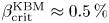 with $\hat {s} = -0.2$
 and $k_y = 0.1$
 when a sufficiently strong ITG is present. It has been suggested that the cause of this destabilization of KBMs at small $\beta$
 is an effect of ion magnetic drift resonance (Hirose et al. Reference Hirose, Zhang and Elia1995; Hirose & Elia Reference Hirose and Elia1996; Chen et al. Reference Chen, Yu, Ma, Shi, Li, Shi, Du, Ji, Jiang and Yu2018). Thermal ions couple to and exchange energy with the drift wave via the geodesic curvature of the magnetic geometry. There are also recent reports of KBMs in experiments which exhibit low negative magnetic shear (Chen et al. Reference Chen, Ma, Li, Shi, Du, Jiang, Yu, Yuan, Li and Yang2016, Reference Chen, Yu, Ma, Shi, Li, Shi, Du, Ji, Jiang and Yu2018), where it is suggested that the same ion-magnetic-drift effect is responsible for the destabilization at small $\beta$
 .
A preliminary, lowest-order analysis of the ion-magnetic-drift resonance condition, derived using a two-fluid model that accounts for kinetic effects, given in Hirose & Elia (Reference Hirose and Elia1996):

where $\omega _{D{i}} = 2 c T_{i} / (eB^3) (\boldsymbol {\nabla } B \times \boldsymbol {B}) \boldsymbol {\cdot } \boldsymbol {k}_\perp$ , suggests that the KBM frequencies observed in the present work exhibit good agreement with that required for exact resonance. Note the different sign used in the parentheses in (4.1) due to the difference in sign convention used for $\omega$
 here relative to Hirose & Elia (Reference Hirose and Elia1996). Taking $T_{e} / T_{i} = 1$
 , $2cT_{i} / (eB) \rightarrow c_{s} \rho _{s}$
 and $\boldsymbol {\nabla } B \rightarrow B/a$
 , the ion-magnetic-drift frequency can be written as $\omega _{D{i}} / (c_{s} / a) \approx k_\perp \rho _{s}$
 . After computing an eigenmode average for $k_\perp \rho _{s}$
 which accounts for geometry, given by

where $g^{xx}$ , $g^{xy}$
 and $g^{yy}$
 are magnetic geometry elements, $\omega _{D{i}} / (c_{s} / a) \approx \langle k_\perp \rho _{s} \rangle$
 yields a normalized ion-magnetic-drift frequency $\omega _{D{i}} = 0.266$
 for ($k_x = 0$
 , $k_y=0.2$
 ). Using this value for $\omega _{D{i}}$
 , one can evaluate (4.1) to determine the resonant mode frequency. The resonant frequency is $\omega \approx 0.724$
 for ($k_x = 0$
 , $k_y=0.2$
 ). The resonant frequency calculated here is in agreement with the dominant KBM real frequency in figure 4 at $k_y = 0.2$
 , where $\omega _r \approx 0.72$
 . This constitutes quantitative evidence that the ion-magnetic-drift resonance is likely playing an important role in the dynamics. A more thorough analysis of the ion-magnetic-drift resonance phenomenon will be left to future work.
In support of the concept that ion dynamics is of particular importance to KBM behaviour in HSX geometry, figure 16 shows $\beta _{\rm crit}^{\rm KBM}$ as a function of $k_y$
 , similar to figure 3, but with different gradients. Keeping the sum of the gradients as well as $a / L_{T{e}}$
 constant, setting $a / L_{T{i}} = 0$
 and increasing $a / L_{T{\rm n}}$
 accordingly, one observes both a roughly five-fold increase in $\beta _{\rm crit}^{\rm KBM}$
 at $k_y = 0.1$
 and that $\beta _{\rm crit}^{\rm KBM}$
 no longer dips as far below $\beta _{\rm crit}^{\rm MHD}$
 . Below $k_y = 0.025$
 , $\beta _{\rm crit}^{\rm KBM}$
 is difficult to ascertain, as a mode that drifts in the electron diamagnetic direction with even $\varPhi$
 parity and odd $A_\parallel$
 parity dominates over the relevant $\beta$
 range and eigenvalue calculations are impractical at such small values of $k_y$
 . This result constitutes further evidence that ion dynamics is of particular importance to KBM behaviour in HSX.
The $\beta _{\rm crit}^{\rm KBM}$ spectrum for HSX with a stronger density gradient contribution compared with figure 3: $a / L_n = 2.5$
 , $a / L_{T{i}} = 0$
 and $a / L_{T{e}} = 1$
 . Since two particle species are used, the sum of the gradients is $2.5 + 2.5 + 1 = 6$
 , which is equal to the sum of the gradients in figure 3. Note that the KBM limit is now closer to $\beta _{\rm crit}^{\rm MHD}$
 as $k_y \to 0$
 .

Regarding scalings of KBM turbulence and confinement at high $\beta$ , linear computations alone are often insufficient to predict nonlinear trends, particularly at low $\hat {s}$
 , as discussed in, for example, Hegna, Terry & Faber (Reference Hegna, Terry and Faber2018) and McKinney et al. (Reference McKinney, Pueschel, Faber, Hegna, Talmadge, Anderson, Mynick and Xanthopoulos2019). While more research on this topic in the context of KBMs is required, the low heat fluxes in figure 6 show both that the strong linear KBM drive at low magnetic shear does not produce corresponding fluxes and that electromagnetic stabilization of the heat flux relative to the electrostatic case can be shown. More explicitly, dominant linear growth rates alone are poor predictors of nonlinear heat fluxes at finite $\beta$
 .
Analyses similar to the ones conducted above for HSX were also carried out for both H-J and a circular axisymmetric geometry. The H-J case, a configuration with similarly low average magnetic shear ($\hat {s} \approx 0.028$ ), also exhibits a small $\beta _{\rm crit}^{\rm KBM} \approx 0.14\,\%$
 at $k_y = 0.1$
 , as evidenced by figure 17. This value of $\beta _{\rm crit}^{\rm KBM}$
 verifies calculations carried out using the GKV code of the same H-J equilibrium using the same gradient values (Maeyama et al. Reference Maeyama, Ishizawa, Watanabe, Nakajima, Tsuji-lio and Tsutsui2013; Ishizawa et al. Reference Ishizawa, Kishimoto, Watanabe, Sugama, Tanaka, Satake, Kobayashi, Nagasaki and Nakamura2017). Also note that there is a slight increase in the ITG growth rates as $\beta \to \beta _{\rm crit}^{\rm KBM}$
 , i.e. no linear electromagnetic stabilization occurs. One particular benefit of including H-J in this analysis is to highlight the fact that the linear and nonlinear KBM dynamics observed numerically in HSX are not simply the product of an aspect of the magnetic geometry that is unique to HSX, but rather are indicative of KBM behaviour in a broader class of magnetic equilibria which exhibit small average magnetic shear.
Growth rate $\gamma$ as a function of $\beta$
 for H-J at $k_y = 0.1$
 with the following normalized (to major radius) gradients: $R_0 / L_{T{i}} = 13$
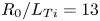 , $R_0 / L_{T{e}} = 17$
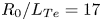 and $R_0 / L_{n} = 9.3$
 . The ITG modes (triangles) dominate below $\beta _{\rm crit}^{\rm KBM}$
 and KBMs (diamonds) dominate above $\beta _{\rm crit}^{\rm KBM}$
 . Note that $\beta _{\rm crit}^{\rm KBM} = 0.14\,\%$
 , shown in red, is comparable to that for HSX for the same binormal wavenumber.

A shifted-circle tokamak geometry with a low negative average magnetic shear $\hat {s} \approx -0.05$ also exhibits $\beta _{\rm crit}^{\rm KBM}$
 spectra and eigenvalue characteristics similar to those for HSX, as shown in figure 18. Note the similarities in the $\beta _{\rm crit}^{\rm KBM}$
 spectrum between HSX and the circular tokamak with low negative average magnetic shear. Both curves are non-monotonic and have a minimum at $k_y = 0.1$
 with a very small critical $\beta _{\rm crit}^{\rm KBM} \approx 0.1\,\%$
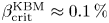 , as shown in figure 18(a). It is also worth noting that the low-$k_y$
 behaviour of $\beta _{\rm crit}^{\rm KBM}$
 in $s$
 –$\alpha$
 is insensitive to the use of a self-consistent equilibrium relative to the high-$k_y$
 behaviour. The subdominant mode landscape for the circular tokamak is also qualitatively consistent with the HSX results, as two distinct clouds of modes are present, an ITG and a KBM branch, as shown in figure 18. However, one key difference between the subdominant mode spectra for HSX and the circular tokamak is the presence of only a single ballooning-parity and tearing-parity KBM branch for the circular tokamak case. The single KBM branch in the axisymmetric case resembles the branch of KBMs centred at the outboard midplane for HSX.
The $\beta _{\rm crit}^{\rm KBM}$ spectrum (a) and the subdominant mode spectrum at $k_y = 0.2$
 and $\beta = 0.8\,\%$
 (b) for an $\hat {s} = -0.052$
 circular tokamak ($s$
 –$\alpha$
 ) geometry. (a) There are two curves: one for the case when $\alpha _{\rm MHD} = 0$
 (red squares), where the equilibrium and Gene $\beta$
 are not self-consistent; and a second for the case when $\alpha _{\rm MHD}$
 is such that both the equilibrium and Gene $\beta$
 are the same (black triangles). (b) The two distinct subdominant ITG (crosses) and KBM (diamonds) clouds are also present in the circular tokamak case. However, there is only a single KBM branch in this case versus the two that were present in HSX.

In summary, both H-J and a circular axisymmetric geometry with $\hat {s} \approx -0.05$ exhibit KBM behaviour similar to that in HSX, providing strong evidence that the relatively weak averaged magnetic shear is an important factor in determining the KBM dynamics.
5. Conclusions
Gyrokinetic electromagnetic simulations of HSX, H-J and a circular tokamak have been presented, showing that KBMs can be excited at a critical $\beta _{\rm crit}^{\rm KBM}$ that is considerably smaller than the critical $\beta$
 for ideal MHD ballooning. This difference is associated with the relatively low average magnetic shear of these configurations. While one might expect this to bode poorly for the performance of low-average-shear magnetic equilibria, nonlinear simulations of HSX show that saturation is achievable with $\beta _{\rm crit}^{\rm KBM} < \beta < \beta _{\rm crit}^{\rm MHD}$
 and that a significant reduction in transport is observed relative to the $\beta \approx 0$
 case. However, saturation only occurs when the minimum binormal wavenumber $k_y^{\rm min} \rho _{s}$
 of the system is stable to KBMs. One possible explanation of this result is that the nonlinear transfer of energy from the strongly driven KBMs in the binormal wavenumber range $0.1 < k_y \rho _{s} < 0.2$
 to stable modes with $k_y \rho _{s} < 0.1$
 in Fourier space is possible and allows for saturation when the condition that $k_y^{\rm min} \rho _{s}$
 is stable to KBMs is met.
The KBM subdominant mode spectrum of HSX is qualitatively different from what one would observe in an $\hat {s} \sim 1$ tokamak, as HSX exhibits two families of unstable KBMs, whereas there is generally only a single unstable KBM in the high-$\hat {s}$
 tokamak case. With low $\hat {s}$
 , KBMs are more extended along the field line, allowing such modes to access free energy in the gradients via the bad curvature regions away from the outboard midplane of a given field line. As a consequence, KBMs can peak at finite ballooning angle, and even tearing-parity KBMs (TKBMs in the nomenclature of Pueschel et al. (Reference Pueschel, Hatch, Ernst, Guttenfelder, Terry, Citrin and Connor2019)) are found. With respect to $\hat {s}$
 , $\beta _{\rm crit}^{\rm KBM}$
 increases monotonically, regardless of the sign of the average magnetic shear. This is consistent with the fact that stronger magnetic shear tends to stabilize drift waves.
A number of nonlinear analyses have also been conducted here which highlight the importance of KBMs in the nonlinear dynamics. Heat flux spectra shown in figure 7 highlight that KBM transport dominates the dynamics when KBMs are destabilized linearly, even if KBM growth rates are subdominant to ITG growth rates. A comparison of dominant linear KBM real frequencies and nonlinear frequencies shows good agreement in the KBM-dominated $k_y$ range. This constitutes evidence that KBMs are significantly contributing to the nonlinear state. Additionally, an analysis of nonlinear energy transfer shows that KBMs play an integral role in the energy transfer dynamics, even more so than zonal modes, further highlighting the fact that the nonlinear state indeed shows signs of both ITG and KBM drive. An investigation of how the electrostatic ion heat flux changes as a function of $\beta$
 shows a decrease in heat flux as $\beta$
 increases until $\beta$
 is sufficiently close to $\beta _{\rm crit}^{\rm KBM}(k_y = k_y^{\rm min})$
 , showing both the improved nonlinear behaviour relative to linear $\beta _{\rm crit}^{\rm KBM}$
 predictions and the steep increase in fluxes at large values of $\beta \gg \beta ^{\rm KBM}_{\rm crit}$
 .
The linear characteristics of the low-average-magnetic-shear equilibria presented in this work raise questions regarding the utility of such configurations at the $\beta$ values required for an efficient fusion reactor concept. However, as the nonlinear calculations presented here show, nonlinear dynamics can overcome poor linear KBM properties such as the increase in total heat flux generally associated with $\beta > \beta _{\rm crit}^{\rm KBM}$
 , and nonlinear fluxes in HSX even decrease as $\beta$
 increases above $\beta _{\rm crit}^{\rm KBM}(k_y = 0.1)$
 , as shown in figure 13, until $\beta \approx 0.6\,\%$
 . It is important to keep such KBM saturation physics in mind during efforts to optimize stellarator equilibria at reactor-relevant $\beta$
 values. Lastly, the fact that in the present simulations achieving saturation depends critically on $\beta _{\rm crit}^{\rm KBM}(k_y=k_y^{\rm min})$
 , it is possible that the value of $\rho ^\star = \rho _{s} / a$
 – and thus the KBM threshold at $n = 1$
 – of a low-magnetic-shear confinement device may affect the achievable plasma $\beta$
 . However, future investigation will need to determine whether this effect survives in more realistic simulation frameworks, in particular when retaining global profile effects.
Acknowledgements
The authors thank K. Aleynikova, M. Kotschenreuther and T.B. Cote for fruitful discussions.
Editor Paolo Ricci thanks the referees for their advice in evaluating this article.
Funding
This work was supported by the US Department of Energy, Office of Science, Fusion Energy Sciences (award numbers DE-FG02-93ER54222, DE-FG02-04ER54742, DE-FG02-89ER53291 and DE-FG02-99ER54546). Computing time was provided through the National Energy Research Scientific Computing Center, a DOE Office of Science User Facility (grant number DE-AC02-05CH11231).
Declaration of interests
The authors report no conflict of interest.



