1 Introduction
The fluid motion in a porous medium in the absence of inertia can be described by the incompressible Brinkman equations (Brinkman Reference Brinkman1949)
 $$\begin{eqnarray}0=\unicode[STIX]{x1D735}\boldsymbol{\cdot }\boldsymbol{u},\quad \frac{\unicode[STIX]{x1D707}}{k}\boldsymbol{u}=-\unicode[STIX]{x1D735}p+\frac{\unicode[STIX]{x1D707}}{\unicode[STIX]{x1D719}}\unicode[STIX]{x0394}\boldsymbol{u}+\boldsymbol{g},\end{eqnarray}$$
where
 $\boldsymbol{u}$
is the average fluid velocity,
 $p$
is the averaged pressure,
 $\unicode[STIX]{x1D707}$
is the fluid viscosity,
 $k$
is the permeability of the porous medium,
 $\unicode[STIX]{x1D719}$
is a dimensionless porosity and
 $\boldsymbol{g}$
is an external force per unit volume. The equations were originally written in terms of an effective viscosity as a coefficient in the viscous term. Since then it has been shown (Chandesris & Jamet Reference Chandesris and Jamet2006) that using volume averaging and assuming a homogeneous porous region results in an effective viscosity equal to the fluid viscosity divided by the porosity,
 $\unicode[STIX]{x1D707}/\unicode[STIX]{x1D719}$
, so we use this formulation here. When the permeability of the medium is small,
 $k\ll 1$
, the viscous term can be neglected and the equation reduces to Darcy’s law. On the other hand, in the limit of large permeability,
 $k\rightarrow \infty$
, the Brinkman equations reduce to the Stokes equations for a fluid without microscopic obstructions.
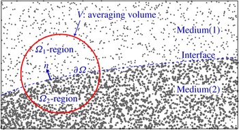
The focus of this work is to derive the boundary integral formulation for the flow in a domain where a porous region described by
 $(k_{1},\unicode[STIX]{x1D719}_{1})$
surrounds another porous region described by
 $(k_{2},\unicode[STIX]{x1D719}_{2})$
, where the flow in the media is described by the Brinkman equations. In this case the interface does not move or deform since a porous medium is formed of fixed solid particles with pores in between. In addition, the viscosities in both porous media must be the same, since the same fluid is passing through the pores of both media. While there is much work on the flow through a porous medium surrounded by a viscous fluid described by the Stokes equation, to our knowledge the boundary integral formulation for the Brinkman–Brinkman problem is new.
Structures composed of a porous medium adjacent to a fluid flow are often seen in industrial processes (wastewater treatment, filtration, thermal insulation), environmental phenomena (groundwater pollution, sea water flow above coral reefs) and biological settings (bacterial biofilms) (Manem & Rittmann Reference Manem and Rittmann1992; Costerton, Stewart & Greenberg Reference Costerton, Stewart and Greenberg1999; Goyeau et al. Reference Goyeau, Lhuillier, Gobin and Velarde2003; Lowe et al. Reference Lowe, Shavit, Falter, Koseff and Monismith2008; Bear & Cheng Reference Bear and Cheng2010). This case of a porous medium surrounded by a Stokes flow has been a topic of active investigation with the main goal of deriving appropriate boundary conditions at the interface (Beavers & Joseph Reference Beavers and Joseph1967; Beavers, Sparrow & Magnuson Reference Beavers, Sparrow and Magnuson1970; Richardson Reference Richardson1971; Saffman Reference Saffman1971; Taylor Reference Taylor1971; Neale & Nader Reference Neale and Nader1974; Howes & Whitaker Reference Howes and Whitaker1985; Ochoa-Tapia Reference Ochoa-Tapia1995; Goyeau et al. Reference Goyeau, Lhuillier, Gobin and Velarde2003; Chandesris & Jamet Reference Chandesris and Jamet2006; Valdés-Parada, Goyeau & Ochoa-Tapia Reference Valdés-Parada, Goyeau and Ochoa-Tapia2007; Tlupova & Cortez Reference Tlupova and Cortez2009; Valdés-Parada et al. Reference Valdés-Parada, Alvarez-Ramirez, Goyeau and Ochoa-Tapia2009, Reference Valdés-Parada, Aguliar-Madera, Ochoa-Tapia and Goyeau2013).
Not all of these models use the Brinkman equation; some use Darcy’s law in the porous medium. Based on the equations used in the porous domain, an appropriate set of boundary conditions has to be imposed at the fluid–porous interface. One interface condition that follows from the incompressibility property of the flow is the continuity of the normal velocity. Beavers and Joseph applied Darcy’s law in a porous domain where a viscous fluid flows in a horizontal channel bounded by a wall on the top and a porous layer on the bottom, with a planar dividing interface between the fluid and porous regions. They used experimental data to propose a semi-empirical slip boundary condition (Beavers & Joseph Reference Beavers and Joseph1967)
 $$\begin{eqnarray}\frac{\unicode[STIX]{x2202}u_{\unicode[STIX]{x1D70F}}^{\,f}}{\unicode[STIX]{x2202}\boldsymbol{n}}=\frac{\unicode[STIX]{x1D709}}{\sqrt{k}}(u_{\unicode[STIX]{x1D70F}}^{\,f}-u_{\unicode[STIX]{x1D70F}}^{\,p})\end{eqnarray}$$
at the interface, where the subscript
 $\unicode[STIX]{x1D70F}$
indicates the tangential component of the interface velocity and
 $\unicode[STIX]{x1D709}$
is a dimensionless adjustable slip coefficient, which can be chosen to match results with the experimental data. The superscripts
 $f$
and
 $p$
refer to the fluid and the porous medium, respectively. Later, condition (1.2) was justified theoretically (Saffman Reference Saffman1971). It was discovered that the value of the slip coefficient
 $\unicode[STIX]{x1D709}$
is strongly dependent on the local geometry of the interface (Beavers et al.
Reference Beavers, Sparrow and Magnuson1970; Richardson Reference Richardson1971; Taylor Reference Taylor1971).
When describing a porous medium flow by the Brinkman equations instead of Darcy’s law, more boundary conditions are required at the interface due to the spatial derivatives of the velocity. Continuity of both the velocity and the stress have been used at the interface (Neale & Nader Reference Neale and Nader1974; Kohr, Wendland & Sekhar Reference Kohr, Wendland and Sekhar2009; Chen, Gunzburger & Wang Reference Chen, Gunzburger and Wang2010). The approach taken by Ochoa-Tapia & Whitaker (Reference Ochoa-Tapia and Whitaker1995) is to impose a jump condition on the tangential components of the stress using the volume-averaged method on the Stokes equation at the interface:
 $$\begin{eqnarray}(\unicode[STIX]{x1D64F}^{\,p}\boldsymbol{n})\boldsymbol{\cdot }\unicode[STIX]{x1D749}-(\unicode[STIX]{x1D64F}^{\,f}\boldsymbol{n})\boldsymbol{\cdot }\unicode[STIX]{x1D749}=\unicode[STIX]{x1D6FD}\frac{\unicode[STIX]{x1D707}}{\sqrt{k}}(\boldsymbol{u}^{\,p}\boldsymbol{\cdot }\unicode[STIX]{x1D749}),\end{eqnarray}$$
where
 $$\begin{eqnarray}\displaystyle & \unicode[STIX]{x1D64F}^{\,f}=-p^{\,f}\unicode[STIX]{x1D644}+\unicode[STIX]{x1D707}([\unicode[STIX]{x1D735}\boldsymbol{u}^{\,f}]+[\unicode[STIX]{x1D735}\boldsymbol{u}^{\,f}]^{t}), & \displaystyle\end{eqnarray}$$
 $$\begin{eqnarray}\displaystyle & \displaystyle \unicode[STIX]{x1D64F}^{\,p}=-p^{\,p}\unicode[STIX]{x1D644}+\frac{\unicode[STIX]{x1D707}}{\unicode[STIX]{x1D719}}([\unicode[STIX]{x1D735}\boldsymbol{u}^{\,p}]+[\unicode[STIX]{x1D735}\boldsymbol{u}^{\,p}]^{t}) & \displaystyle\end{eqnarray}$$
and
 $\unicode[STIX]{x1D6FD}$
is an adjustable stress jump coefficient. The superscript
 $t$
in (1.5) denotes the transpose operator. The jump condition (1.3) becomes
 $$\begin{eqnarray}\displaystyle \frac{\unicode[STIX]{x1D707}}{\unicode[STIX]{x1D719}}\frac{\unicode[STIX]{x2202}u_{\unicode[STIX]{x1D70F}}^{\,p}}{\unicode[STIX]{x2202}\boldsymbol{n}}-\frac{\unicode[STIX]{x2202}u_{\unicode[STIX]{x1D70F}}^{\,f}}{\unicode[STIX]{x2202}\boldsymbol{n}}=\unicode[STIX]{x1D6FD}\frac{\unicode[STIX]{x1D707}}{\sqrt{k}}u_{\unicode[STIX]{x1D70F}}^{\,p}. & & \displaystyle\end{eqnarray}$$
The determination of the parameter
 $\unicode[STIX]{x1D6FD}$
remains the subject of intense research activity. Introducing a thin transition layer between the fluid and porous regions, an expression for
 $\unicode[STIX]{x1D6FD}$
was derived based on the variation in velocity, the geometry of the interface and the variations of the porous material properties (Goyeau et al.
Reference Goyeau, Lhuillier, Gobin and Velarde2003). One difficulty with this expression lies on the fact that the expression for
 $\unicode[STIX]{x1D6FD}$
depends on the velocity, which is an unknown of the problem. To reduce the complexity in determining
 $\unicode[STIX]{x1D6FD}$
, Chandesris & Jamet (Reference Chandesris and Jamet2006) used matched asymptotics to derive the interface jump condition
 $$\begin{eqnarray}\displaystyle & u_{\unicode[STIX]{x1D70F}}^{\,f}=u_{\unicode[STIX]{x1D70F}}^{\,p}, & \displaystyle\end{eqnarray}$$
 $$\begin{eqnarray}\displaystyle & \displaystyle \frac{\unicode[STIX]{x2202}u_{\unicode[STIX]{x1D70F}}^{\,p}}{\unicode[STIX]{x2202}\boldsymbol{n}}-\frac{\unicode[STIX]{x2202}u_{\unicode[STIX]{x1D70F}}^{\,f}}{\unicode[STIX]{x2202}\boldsymbol{n}}=\frac{\unicode[STIX]{x1D6FD}}{\sqrt{k}}u_{\unicode[STIX]{x1D70F}}^{\,p}, & \displaystyle\end{eqnarray}$$
where
 $\unicode[STIX]{x1D6FD}$
is given by (Chandesris & Jamet Reference Chandesris and Jamet2006)
 $$\begin{eqnarray}\unicode[STIX]{x1D6FD}=\frac{\unicode[STIX]{x1D6FF}}{\sqrt{k}}\left(\unicode[STIX]{x1D6FE}-\unicode[STIX]{x1D706}\frac{2(1+\unicode[STIX]{x1D70E}\sqrt{\unicode[STIX]{x1D719}})}{\unicode[STIX]{x1D70E}(\unicode[STIX]{x1D70E}+2\sqrt{\unicode[STIX]{x1D719}})}\right).\end{eqnarray}$$
The expression involves the transition layer thickness
 $\unicode[STIX]{x1D6FF}$
and
 $\unicode[STIX]{x1D70E}=1/\sqrt{Da}$
where
 $Da=k/L^{2}$
is the Darcy number which relates the permeability
 $k$
and the length scale
 $L$
of the problem. The quantities
 $\unicode[STIX]{x1D6FE}$
and
 $\unicode[STIX]{x1D706}$
depend on
 $k$
and
 $\unicode[STIX]{x1D719}$
in the transition region. For example, if we assume
 $\unicode[STIX]{x1D719}$
and
 $1/k$
transition linearly, then (Chandesris & Jamet Reference Chandesris and Jamet2006)
 $$\begin{eqnarray}\unicode[STIX]{x1D6FE}=\frac{1-\unicode[STIX]{x1D719}}{6},\quad \unicode[STIX]{x1D706}=0,\end{eqnarray}$$
or if those variations are following a hyperbolic tangent, then
 $$\begin{eqnarray}\unicode[STIX]{x1D6FE}=\frac{1-\unicode[STIX]{x1D719}}{2},\quad \unicode[STIX]{x1D706}=0.\end{eqnarray}$$
In any case, the parameters
 $\unicode[STIX]{x1D6FF}$
,
 $\unicode[STIX]{x1D6FE}$
and
 $\unicode[STIX]{x1D706}$
must be determined for each particular problem.
Valdés-Parada et al. (Reference Valdés-Parada, Goyeau and Ochoa-Tapia2007) provided an interface stress jump condition that does not include the parameter
 $\unicode[STIX]{x1D6FD}$
. They predicted
 $\unicode[STIX]{x1D6FD}$
in terms of other variables by assuming a functional form for
 $\unicode[STIX]{x1D719}$
and estimating empirically the permeability in the porous region. Finally, they presented an expression for the mixed stress tensor in terms of porosity and length scale of the problem, approximating
 $\unicode[STIX]{x1D6FD}$
as
 $$\begin{eqnarray}\displaystyle \unicode[STIX]{x1D6FD}=\frac{2\unicode[STIX]{x1D719}^{3/2}}{3\sqrt{\unicode[STIX]{x1D6FE}}(1+\unicode[STIX]{x1D719})^{3}} & & \displaystyle\end{eqnarray}$$
assuming that the porous medium was composed of equally spaced spheres or cylinders of a fixed diameter. The parameter
 $\unicode[STIX]{x1D6FE}$
assumes different expressions based on the permeability estimate and experimental data. Therefore, equation (1.12) provides an expression for
 $\unicode[STIX]{x1D6FD}$
that is only related to the porosity
 $\unicode[STIX]{x1D719}$
and not to the characteristics of the microstructure (Valdés-Parada et al.
Reference Valdés-Parada, Goyeau and Ochoa-Tapia2007). Generally, for the Stokes–Brinkman case, it is most common to assume continuity of the velocity at the interface (no slip) (Alazmi & Vafai Reference Alazmi and Vafai2000).
Larson & Higdon (Reference Larson and Higdon1986, Reference Larson and Higdon1987) investigated the case of a porous medium in a viscous fluid at a microscopic level by considering semi-infinite lattice of cylinders in various arrangements. The boundary integral method was used to solve the Stokes equation around the cylinders. They conclude that the small-scale flow near the surface of the porous particle is sensitive to changes in the porous medium structure. Later Sahraoui & Kaviany (Reference Sahraoui and Kaviany1992) performed a related study focused on the appropriate location of the interface when modelling the detailed flows around particles. They also discuss the slip velocity interface condition in the context of Darcy’s law and the velocity continuity in the context of the Brinkman equation.
In the next sections we derive the boundary integral formulation for the case of a porous medium surrounded by another porous medium with different properties where the fluid flow in both media are described by the Brinkman equations. Accounting for the possibility of a jump in the tangential stress at the interface, we develop interface conditions in a form similar to (1.3), which can also be used with
 $\unicode[STIX]{x1D6FD}=0$
to include the assumption of continuous stress. The final expressions generalize the known case of a porous medium surrounded by a Stokes flow in the limit of infinite permeability in the outside medium. The final section shows simulated flows in two dimensions that exemplify the results of the formulation.
2 Mathematical background
In the regime of highly viscous flows or very small length scales, an appropriate description of the fluid motion in the porous region is given by the Brinkman equations (1.1), where the permeability
 $k$
is a measure of the ability of the porous medium to allow fluid to pass through the pores. Considering a control volume,
 $V$
, in the porous medium,
 $\unicode[STIX]{x1D719}$
is defined as the fraction of the volume of the void space filled by the fluid,
 $V_{f}$
, to the control volume,
 $V$
, i.e.
 $\unicode[STIX]{x1D719}=V_{f}/V$
. Therefore, it is a number between 0 and 1.
If we denote the non-dimensional operators and quantities by an asterisk superscript, and use
 $L$
and
 $U$
as representative length and velocity scales of the problem, then the dimensionless form of the equations is
 $$\begin{eqnarray}\displaystyle & 0=\unicode[STIX]{x1D735}\boldsymbol{\cdot }\boldsymbol{u}^{\ast }, & \displaystyle\end{eqnarray}$$
 $$\begin{eqnarray}\displaystyle & \displaystyle \frac{\unicode[STIX]{x1D6FC}^{2}}{\unicode[STIX]{x1D719}}\boldsymbol{u}^{\ast }=-\unicode[STIX]{x1D735}p^{\ast }+\frac{1}{\unicode[STIX]{x1D719}}\unicode[STIX]{x0394}\boldsymbol{u}^{\ast }+\boldsymbol{g}^{\ast }, & \displaystyle\end{eqnarray}$$
where the dimensionless pressure and force density are
 $p^{\ast }=L/\unicode[STIX]{x1D707}Up$
and
 $\boldsymbol{g}^{\ast }=L^{2}/\unicode[STIX]{x1D707}U\boldsymbol{g}$
. The parameter
 $\unicode[STIX]{x1D6FC}^{2}$
is defined as
 $\unicode[STIX]{x1D6FC}^{2}=\unicode[STIX]{x1D719}L^{2}/k=\unicode[STIX]{x1D719}/Da$
where the dimensionless number
 $Da$
is the Darcy number defined as
 $$\begin{eqnarray}Da=\frac{k}{L^{2}}.\end{eqnarray}$$
From (2.2), it is clear that when the permeability
 $k$
approaches infinity, the entire volume is occupied by the fluid so that
 $(\unicode[STIX]{x1D6FC},\unicode[STIX]{x1D719})\rightarrow (0,1)$
and the Brinkman equation reduces to the Stokes equation. We will consider the flow in a domain consisting of a porous medium
 $\unicode[STIX]{x1D6FA}_{2}$
with properties
 $(\unicode[STIX]{x1D6FC}_{2},\unicode[STIX]{x1D719}_{2})$
surrounded by another porous medium
 $\unicode[STIX]{x1D6FA}_{1}$
with properties
 $(\unicode[STIX]{x1D6FC}_{1},\unicode[STIX]{x1D719}_{1})$
, as shown in figure 1.
Schematic of the Brinkman–Brinkman problem.

3 Boundary integral formulation
To derive the boundary integral formulas, we apply the following Brinkman reciprocal identity
 $$\begin{eqnarray}u_{j}(\boldsymbol{x})\unicode[STIX]{x1D6FF}(\boldsymbol{x}-\boldsymbol{x}_{0})=\frac{\unicode[STIX]{x2202}}{\unicode[STIX]{x2202}x_{k}}[\unicode[STIX]{x1D719}\unicode[STIX]{x1D61A}_{ij}(\boldsymbol{x},\boldsymbol{x}_{0};\unicode[STIX]{x1D6FC})\unicode[STIX]{x1D70E}_{ik}(\boldsymbol{x})-u_{i}(\boldsymbol{x})\unicode[STIX]{x1D61B}_{ijk}(\boldsymbol{x},\boldsymbol{x}_{0};\unicode[STIX]{x1D6FC})],\end{eqnarray}$$
where
 $\unicode[STIX]{x1D61A}_{ij}$
and
 $\unicode[STIX]{x1D61B}_{ijk}$
are the fundamental solution of the Brinkman equation (referred to as a Brinkmanlet) and the Brinkman stress tensor defined as
 $$\begin{eqnarray}\unicode[STIX]{x1D61A}_{ij}(\boldsymbol{x},\boldsymbol{x}_{0};\unicode[STIX]{x1D6FC})=H_{1}^{b}(r)\unicode[STIX]{x1D6FF}_{ij}+H_{2}^{b}(r)(x_{i}-x_{0i})(x_{j}-x_{0j}),\end{eqnarray}$$
 $$\begin{eqnarray}\displaystyle \unicode[STIX]{x1D61B}_{ijk}(\boldsymbol{x},\boldsymbol{x}_{0};\unicode[STIX]{x1D6FC}) & = & \displaystyle W_{1}^{b}(r)\;(x_{j}-x_{0j})\unicode[STIX]{x1D6FF}_{ik}+W_{2}^{b}(r)[(x_{k}-x_{0k})\unicode[STIX]{x1D6FF}_{ij}+(x_{i}-x_{0i})\unicode[STIX]{x1D6FF}_{jk}]\nonumber\\ \displaystyle & & \displaystyle +\,W_{3}^{b}(r)(x_{i}-x_{0i})(x_{j}-x_{0j})(x_{k}-x_{0k}).\end{eqnarray}$$
Here,
 $r=|\boldsymbol{x}-\boldsymbol{x}_{0}|$
and the relevant functions in
 $\mathbb{R}^{3}$
are
 $$\begin{eqnarray}\displaystyle & \displaystyle H_{1}^{b}(r)=\frac{\text{e}^{(-\unicode[STIX]{x1D6FC}r)}[\unicode[STIX]{x1D6FC}r(\unicode[STIX]{x1D6FC}r+1)+1]-1}{4\unicode[STIX]{x03C0}\unicode[STIX]{x1D6FC}^{2}r^{3}}, & \displaystyle\end{eqnarray}$$
 $$\begin{eqnarray}\displaystyle & \displaystyle H_{2}^{b}(r)=\frac{\text{e}^{(-\unicode[STIX]{x1D6FC}r)}[-\unicode[STIX]{x1D6FC}r(\unicode[STIX]{x1D6FC}r+3)-3]+3}{4\unicode[STIX]{x03C0}\unicode[STIX]{x1D6FC}^{2}r^{5}}, & \displaystyle\end{eqnarray}$$
 $$\begin{eqnarray}\displaystyle & \displaystyle W_{1}^{b}(r)=-\frac{\unicode[STIX]{x1D6FC}^{2}r^{2}+\text{e}^{-\unicode[STIX]{x1D6FC}r}(2\unicode[STIX]{x1D6FC}r(\unicode[STIX]{x1D6FC}r+3)-6\text{e}^{\unicode[STIX]{x1D6FC}r}+6)}{4\unicode[STIX]{x03C0}\unicode[STIX]{x1D6FC}^{2}r^{5}}, & \displaystyle\end{eqnarray}$$
 $$\begin{eqnarray}\displaystyle & \displaystyle W_{2}^{b}(r)=\frac{\text{e}^{-\unicode[STIX]{x1D6FC}r}(-\unicode[STIX]{x1D6FC}r(\unicode[STIX]{x1D6FC}r(\unicode[STIX]{x1D6FC}r+3)+6)+6\text{e}^{\unicode[STIX]{x1D6FC}r}-6)}{4\unicode[STIX]{x03C0}\unicode[STIX]{x1D6FC}^{2}r^{5}}, & \displaystyle\end{eqnarray}$$
 $$\begin{eqnarray}\displaystyle & \displaystyle W_{3}^{b}(r)=\frac{\text{e}^{-\unicode[STIX]{x1D6FC}r}(\unicode[STIX]{x1D6FC}r(\unicode[STIX]{x1D6FC}r(\unicode[STIX]{x1D6FC}r+6)+15)-15\text{e}^{\unicode[STIX]{x1D6FC}r}+15)}{2\unicode[STIX]{x03C0}\unicode[STIX]{x1D6FC}^{2}r^{7}}, & \displaystyle\end{eqnarray}$$
and in
 $\mathbb{R}^{2}$
the functions are
 $$\begin{eqnarray}\displaystyle & \displaystyle H_{1}^{b}(r)=\frac{-2+\unicode[STIX]{x1D6FC}^{2}r^{2}(K_{0}(r\unicode[STIX]{x1D6FC})+K_{2}(r\unicode[STIX]{x1D6FC}))}{4\unicode[STIX]{x03C0}\unicode[STIX]{x1D6FC}^{2}r^{2}}-C_{0}(\unicode[STIX]{x1D6FC}), & \displaystyle\end{eqnarray}$$
 $$\begin{eqnarray}\displaystyle & \displaystyle H_{2}^{b}(r)=\frac{2-\unicode[STIX]{x1D6FC}^{2}r^{2}K_{2}(\unicode[STIX]{x1D6FC}r)}{2\unicode[STIX]{x03C0}\unicode[STIX]{x1D6FC}^{2}r^{4}}, & \displaystyle\end{eqnarray}$$
 $$\begin{eqnarray}\displaystyle & \displaystyle W_{1}^{b}(r)=\frac{4-2\unicode[STIX]{x1D6FC}^{2}r^{2}K_{2}(r\unicode[STIX]{x1D6FC})-\unicode[STIX]{x1D6FC}^{2}r^{2}}{2\unicode[STIX]{x03C0}\unicode[STIX]{x1D6FC}^{2}r^{4}}, & \displaystyle\end{eqnarray}$$
 $$\begin{eqnarray}\displaystyle & \displaystyle W_{2}^{b}(r)=\frac{4-\unicode[STIX]{x1D6FC}^{2}r^{2}[\unicode[STIX]{x1D6FC}rK_{1}(r\unicode[STIX]{x1D6FC})+2K_{2}(r\unicode[STIX]{x1D6FC})]}{2\unicode[STIX]{x03C0}\unicode[STIX]{x1D6FC}^{2}r^{4}}, & \displaystyle\end{eqnarray}$$
 $$\begin{eqnarray}\displaystyle & \displaystyle W_{3}^{b}(r)=\frac{\unicode[STIX]{x1D6FC}^{3}r^{3}K_{3}(r\unicode[STIX]{x1D6FC})-8}{\unicode[STIX]{x03C0}\unicode[STIX]{x1D6FC}^{2}r^{6}}, & \displaystyle\end{eqnarray}$$
where
 $K_{j}$
is the modified Bessel function of the second kind of order
 $j$
. The constant in the expression for
 $H_{1}^{b}(r)$
is
 $C_{0}(\unicode[STIX]{x1D6FC})=(-1-\ln (\unicode[STIX]{x1D6FC}^{2})-2\unicode[STIX]{x1D6FE}+\ln (4))/8\unicode[STIX]{x03C0}$
and is included so that as
 $\unicode[STIX]{x1D6FC}$
vanishes,
 $\unicode[STIX]{x1D61A}_{ij}(\boldsymbol{x},\boldsymbol{x}_{0};\unicode[STIX]{x1D6FC})$
converges to the fundamental solution of Stokes equations. Since
 $C_{0}(\unicode[STIX]{x1D6FC})$
only appears in
 $H_{1}^{b}(r)$
, equation (3.2) shows that its effect is to produce a constant flow that can be subtracted. In situations where a set of forces that drive the fluid motion have zero net force, the constant
 $C_{0}(\unicode[STIX]{x1D6FC})$
does not have any effect.
Referring to figure 1, let
 $\boldsymbol{x}_{0}\in \unicode[STIX]{x1D6FA}_{1}$
, integrate (3.1) over the domain
 $\unicode[STIX]{x1D6FA}_{1}$
and apply the divergence theorem to obtain
 $$\begin{eqnarray}\displaystyle u_{j}^{(1)}(\boldsymbol{x}_{0}) & = & \displaystyle -\int _{\unicode[STIX]{x2202}\unicode[STIX]{x1D6FA}}\unicode[STIX]{x1D719}_{1}\unicode[STIX]{x1D61A}_{ij}(\boldsymbol{x},\boldsymbol{x}_{0};\unicode[STIX]{x1D6FC}_{1})\unicode[STIX]{x1D70E}_{ik}^{(1)}(\boldsymbol{x})n_{k}(\boldsymbol{x})\,\text{d}\ell (\boldsymbol{x})\nonumber\\ \displaystyle & & \displaystyle +\,\int _{\unicode[STIX]{x2202}\unicode[STIX]{x1D6FA}}u_{i}(\boldsymbol{x})\unicode[STIX]{x1D61B}_{ijk}(\boldsymbol{x},\boldsymbol{x}_{0};\unicode[STIX]{x1D6FC}_{1})n_{k}(\boldsymbol{x})\text{d}\ell (\boldsymbol{x}),\end{eqnarray}$$
where
 $\boldsymbol{n}$
is the unit outward normal vector pointing from the domain
 $\unicode[STIX]{x1D6FA}_{2}$
into the domain
 $\unicode[STIX]{x1D6FA}_{1}$
. Integrating (3.1) over the domain
 $\unicode[STIX]{x1D6FA}_{2}$
while
 $\boldsymbol{x}_{0}\in \unicode[STIX]{x1D6FA}_{1}$
gives
 $$\begin{eqnarray}\displaystyle 0=\int _{\unicode[STIX]{x2202}\unicode[STIX]{x1D6FA}}\unicode[STIX]{x1D719}_{2}\unicode[STIX]{x1D61A}_{ij}(\boldsymbol{x},\boldsymbol{x}_{0};\unicode[STIX]{x1D6FC}_{2})\unicode[STIX]{x1D70E}_{ik}^{(2)}(\boldsymbol{x})n_{k}(\boldsymbol{x})\,\text{d}\ell (\boldsymbol{x})-\int _{\unicode[STIX]{x2202}\unicode[STIX]{x1D6FA}}u_{i}(\boldsymbol{x})\unicode[STIX]{x1D61B}_{ijk}(\boldsymbol{x},\boldsymbol{x}_{0};\unicode[STIX]{x1D6FC}_{2})n_{k}(\boldsymbol{x})\,\text{d}\ell (\boldsymbol{x}).\qquad & & \displaystyle\end{eqnarray}$$
If we define
 $f_{i}^{(1)}=\unicode[STIX]{x1D70E}_{ik}^{(1)}n_{k}$
,
 $f_{i}^{(2)}=\unicode[STIX]{x1D70E}_{ik}^{(2)}n_{k}$
and
 $\unicode[STIX]{x1D706}=\unicode[STIX]{x1D719}_{1}/\unicode[STIX]{x1D719}_{2}$
, then multiplying (3.15) by
 $\unicode[STIX]{x1D706}$
and adding the result to (3.14) gives
 $$\begin{eqnarray}\displaystyle u_{j}^{(1)}(\boldsymbol{x}_{0}) & = & \displaystyle -\unicode[STIX]{x1D719}_{1}\int _{\unicode[STIX]{x2202}\unicode[STIX]{x1D6FA}}[\unicode[STIX]{x1D61A}_{ij}(\boldsymbol{x},\boldsymbol{x}_{0};\unicode[STIX]{x1D6FC}_{1})f_{i}^{(1)}-\unicode[STIX]{x1D61A}_{ij}(\boldsymbol{x},\boldsymbol{x}_{0};\unicode[STIX]{x1D6FC}_{2})f_{i}^{(2)}]\,\text{d}\ell (\boldsymbol{x})\nonumber\\ \displaystyle & & \displaystyle +\,\int _{\unicode[STIX]{x2202}\unicode[STIX]{x1D6FA}}u_{i}(\boldsymbol{x})[\unicode[STIX]{x1D61B}_{ijk}(\boldsymbol{x},\boldsymbol{x}_{0};\unicode[STIX]{x1D6FC}_{1})-\unicode[STIX]{x1D706}\unicode[STIX]{x1D61B}_{ijk}(\boldsymbol{x},\boldsymbol{x}_{0};\unicode[STIX]{x1D6FC}_{2})]n_{k}(\boldsymbol{x})\,\text{d}\ell (\boldsymbol{x}).\end{eqnarray}$$
Following a similar procedure starting with
 $\boldsymbol{x}_{0}\in \unicode[STIX]{x1D6FA}_{2}$
, we can derive a boundary integral representation for the internal flow. The result is
 $$\begin{eqnarray}\displaystyle u_{j}^{(2)}(\boldsymbol{x}_{0}) & = & \displaystyle -\unicode[STIX]{x1D719}_{2}\int _{\unicode[STIX]{x2202}\unicode[STIX]{x1D6FA}}[\unicode[STIX]{x1D61A}_{ij}(\boldsymbol{x},\boldsymbol{x}_{0};\unicode[STIX]{x1D6FC}_{1})f_{i}^{(1)}-\unicode[STIX]{x1D61A}_{ij}(\boldsymbol{x},\boldsymbol{x}_{0};\unicode[STIX]{x1D6FC}_{2})f_{i}^{(2)}]\,\text{d}\ell (\boldsymbol{x})\nonumber\\ \displaystyle & & \displaystyle +\,\int _{\unicode[STIX]{x2202}\unicode[STIX]{x1D6FA}}u_{i}(\boldsymbol{x})\left[\frac{1}{\unicode[STIX]{x1D706}}\unicode[STIX]{x1D61B}_{ijk}(\boldsymbol{x},\boldsymbol{x}_{0};\unicode[STIX]{x1D6FC}_{1})-\unicode[STIX]{x1D61B}_{ijk}(\boldsymbol{x},\boldsymbol{x}_{0};\unicode[STIX]{x1D6FC}_{2})\right]n_{k}(\boldsymbol{x})\,\text{d}\ell (\boldsymbol{x}).\end{eqnarray}$$
Given equations for the fluid velocities in
 $\unicode[STIX]{x1D6FA}_{1}$
and
 $\unicode[STIX]{x1D6FA}_{2}$
respectively, we derive a boundary integral formula for the velocity at the interface by taking the limits of (3.16)–(3.17) as
 $\boldsymbol{x}_{0}\rightarrow \unicode[STIX]{x2202}\unicode[STIX]{x1D6FA}$
from both sides of the interface while imposing the continuity of the velocity. The Brinkman double layer potential
 $$\begin{eqnarray}\int _{\unicode[STIX]{x2202}S}u_{i}(\boldsymbol{x})\unicode[STIX]{x1D61B}_{ijk}(\boldsymbol{x},\boldsymbol{x}_{0};\unicode[STIX]{x1D6FC})n_{k}(\boldsymbol{x})\,\text{d}S(\boldsymbol{x})\end{eqnarray}$$
undergoes a discontinuity across the boundary. In fact
 $$\begin{eqnarray}\displaystyle & & \displaystyle \lim _{\boldsymbol{x}_{0}\rightarrow \unicode[STIX]{x2202}S}\int _{\unicode[STIX]{x2202}S}u_{i}(\boldsymbol{x})\unicode[STIX]{x1D61B}_{ijk}(\boldsymbol{x},\boldsymbol{x}_{0};\unicode[STIX]{x1D6FC})n_{k}(\boldsymbol{x})\,\text{d}S(\boldsymbol{x})\nonumber\\ \displaystyle & & \displaystyle \quad =\pm \frac{1}{2}u_{j}(\boldsymbol{x}_{0})+\int _{\unicode[STIX]{x2202}S}^{\,pv}u_{i}(\boldsymbol{x})\unicode[STIX]{x1D61B}_{ijk}(\boldsymbol{x},\boldsymbol{x}_{0};\unicode[STIX]{x1D6FC})n_{k}(\boldsymbol{x})\,\text{d}S(\boldsymbol{x})\end{eqnarray}$$
(see appendix A for the proof) where the superscript ‘
 $pv$
’ denotes the principal value of the double layer potential (Pozrikidis Reference Pozrikidis1992). The plus sign is applied when the evaluation point
 $\boldsymbol{x}_{0}$
is approaching the boundary from
 $\unicode[STIX]{x1D6FA}_{1}$
, whereas the minus sign is applied when the evaluation point
 $\boldsymbol{x}_{0}$
is approaching the boundary from
 $\unicode[STIX]{x1D6FA}_{2}$
.
Therefore, approaching the interface from outside, equation (3.16) gives
 $$\begin{eqnarray}\displaystyle u_{j}(\boldsymbol{x}_{0}) & = & \displaystyle -\unicode[STIX]{x1D719}_{1}\int _{\unicode[STIX]{x2202}\unicode[STIX]{x1D6FA}}[\unicode[STIX]{x1D61A}_{ij}(\boldsymbol{x},\boldsymbol{x}_{0};\unicode[STIX]{x1D6FC}_{1})f_{i}^{(1)}-\unicode[STIX]{x1D61A}_{ij}(\boldsymbol{x},\boldsymbol{x}_{0};\unicode[STIX]{x1D6FC}_{2})f_{i}^{(2)}]\,\text{d}\ell (\boldsymbol{x})\nonumber\\ \displaystyle & & \displaystyle +\,\int _{\unicode[STIX]{x2202}\unicode[STIX]{x1D6FA}}^{\,pv}u_{i}(\boldsymbol{x})[\unicode[STIX]{x1D61B}_{ijk}(\boldsymbol{x},\boldsymbol{x}_{0};\unicode[STIX]{x1D6FC}_{1})-\unicode[STIX]{x1D706}\unicode[STIX]{x1D61B}_{ijk}(\boldsymbol{x},\boldsymbol{x}_{0};\unicode[STIX]{x1D6FC}_{2})]n_{k}(\boldsymbol{x})\,\text{d}\ell (\boldsymbol{x})\nonumber\\ \displaystyle & & \displaystyle +\,\frac{1}{2}(1-\unicode[STIX]{x1D706})u_{j}(\boldsymbol{x}_{0})\end{eqnarray}$$
and approaching the interface from inside, equation (3.17) gives us
 $$\begin{eqnarray}\displaystyle u_{j}(\boldsymbol{x}_{0}) & = & \displaystyle -\unicode[STIX]{x1D719}_{2}\int _{\unicode[STIX]{x2202}\unicode[STIX]{x1D6FA}}[\unicode[STIX]{x1D61A}_{ij}(\boldsymbol{x},\boldsymbol{x}_{0};\unicode[STIX]{x1D6FC}_{1})\;f_{i}^{(1)}-\unicode[STIX]{x1D61A}_{ij}(\boldsymbol{x},\boldsymbol{x}_{0};\unicode[STIX]{x1D6FC}_{2})f_{i}^{(2)}]\,\text{d}\ell (\boldsymbol{x})\nonumber\\ \displaystyle & & \displaystyle +\int _{\unicode[STIX]{x2202}\unicode[STIX]{x1D6FA}}^{\,pv}u_{i}(\boldsymbol{x})\left[\frac{1}{\unicode[STIX]{x1D706}}\unicode[STIX]{x1D61B}_{ijk}(\boldsymbol{x},\boldsymbol{x}_{0};\unicode[STIX]{x1D6FC}_{1})-\unicode[STIX]{x1D61B}_{ijk}(\boldsymbol{x},\boldsymbol{x}_{0};\unicode[STIX]{x1D6FC}_{2})\right]n_{k}(\boldsymbol{x})\,\text{d}\ell (\boldsymbol{x})\nonumber\\ \displaystyle & & \displaystyle -\,\frac{1}{2}\left(\frac{1}{\unicode[STIX]{x1D706}}-1\right)u_{j}(\boldsymbol{x}_{0}).\end{eqnarray}$$
Thus, multiplying (3.21) by
 $\unicode[STIX]{x1D706}$
and adding the result to (3.20) leads to
 $$\begin{eqnarray}\displaystyle u_{j}(\boldsymbol{x}_{0}) & = & \displaystyle \frac{2}{1+\unicode[STIX]{x1D706}}\left[-\unicode[STIX]{x1D719}_{1}\int _{\unicode[STIX]{x2202}\unicode[STIX]{x1D6FA}}[\unicode[STIX]{x1D61A}_{ij}(\boldsymbol{x},\boldsymbol{x}_{0};\unicode[STIX]{x1D6FC}_{1})f_{i}^{(1)}-\unicode[STIX]{x1D61A}_{ij}(\boldsymbol{x},\boldsymbol{x}_{0};\unicode[STIX]{x1D6FC}_{2})f_{i}^{(2)}]\,\text{d}\ell (\boldsymbol{x})\right.\nonumber\\ \displaystyle & & \displaystyle +\left.\int _{\unicode[STIX]{x2202}\unicode[STIX]{x1D6FA}}^{\,pv}u_{i}(\boldsymbol{x})[\unicode[STIX]{x1D61B}_{ijk}(\boldsymbol{x},\boldsymbol{x}_{0};\unicode[STIX]{x1D6FC}_{1})-\unicode[STIX]{x1D706}\unicode[STIX]{x1D61B}_{ijk}(\boldsymbol{x},\boldsymbol{x}_{0};\unicode[STIX]{x1D6FC}_{2})]n_{k}(\boldsymbol{x})\,\text{d}\ell (\boldsymbol{x})\right].\end{eqnarray}$$
Equations (3.16), (3.17) and (3.22) can be modified to include a uniformly constant ambient flow as follows
 $$\begin{eqnarray}\displaystyle u_{j}^{(1)}(\boldsymbol{x}_{0}) & = & \displaystyle u_{j}^{\infty }-u_{i}^{\infty }\int _{\unicode[STIX]{x2202}\unicode[STIX]{x1D6FA}}[\unicode[STIX]{x1D61B}_{ijk}(\boldsymbol{x},\boldsymbol{x}_{0};\unicode[STIX]{x1D6FC}_{1})-\tilde{\unicode[STIX]{x1D6FC}}^{2}\unicode[STIX]{x1D61B}_{ijk}(\boldsymbol{x},\boldsymbol{x}_{0};\unicode[STIX]{x1D6FC}_{2})]n_{k}(\boldsymbol{x})\,\text{d}\ell (\boldsymbol{x})\nonumber\\ \displaystyle & & \displaystyle -\,\unicode[STIX]{x1D719}_{1}\int _{\unicode[STIX]{x2202}\unicode[STIX]{x1D6FA}}[\unicode[STIX]{x1D61A}_{ij}(\boldsymbol{x},\boldsymbol{x}_{0};\unicode[STIX]{x1D6FC}_{1})f_{i}^{(1)}-\unicode[STIX]{x1D61A}_{ij}(\boldsymbol{x},\boldsymbol{x}_{0};\unicode[STIX]{x1D6FC}_{2})f_{i}^{(2)}]\,\text{d}\ell (\boldsymbol{x})\nonumber\\ \displaystyle & & \displaystyle +\,\int _{\unicode[STIX]{x2202}\unicode[STIX]{x1D6FA}}u_{i}(\boldsymbol{x})[\unicode[STIX]{x1D61B}_{ijk}(\boldsymbol{x},\boldsymbol{x}_{0};\unicode[STIX]{x1D6FC}_{1})-\unicode[STIX]{x1D706}\unicode[STIX]{x1D61B}_{ijk}(\boldsymbol{x},\boldsymbol{x}_{0};\unicode[STIX]{x1D6FC}_{2})]n_{k}(\boldsymbol{x})\;\text{d}\ell (\boldsymbol{x}),\end{eqnarray}$$
 $$\begin{eqnarray}\displaystyle u_{j}^{(2)}(\boldsymbol{x}_{0}) & = & \displaystyle \frac{1}{\unicode[STIX]{x1D706}}\left(\tilde{\unicode[STIX]{x1D6FC}}^{2}u_{j}^{\infty }-u_{i}^{\infty }\int _{\unicode[STIX]{x2202}\unicode[STIX]{x1D6FA}}[\unicode[STIX]{x1D61B}_{ijk}(\boldsymbol{x},\boldsymbol{x}_{0};\unicode[STIX]{x1D6FC}_{1})-\tilde{\unicode[STIX]{x1D6FC}}^{2}\unicode[STIX]{x1D61B}_{ijk}(\boldsymbol{x},\boldsymbol{x}_{0};\unicode[STIX]{x1D6FC}_{2})]n_{k}(\boldsymbol{x})\,\text{d}\ell (\boldsymbol{x})\right.\nonumber\\ \displaystyle & & \displaystyle -\,\unicode[STIX]{x1D719}_{1}\int _{\unicode[STIX]{x2202}\unicode[STIX]{x1D6FA}}[\unicode[STIX]{x1D61A}_{ij}(\boldsymbol{x},\boldsymbol{x}_{0};\unicode[STIX]{x1D6FC}_{1})f_{i}^{(1)}-\unicode[STIX]{x1D61A}_{ij}(\boldsymbol{x},\boldsymbol{x}_{0};\unicode[STIX]{x1D6FC}_{2})f_{i}^{(2)}]\,\text{d}\ell (\boldsymbol{x})\nonumber\\ \displaystyle & & \displaystyle +\left.\int _{\unicode[STIX]{x2202}\unicode[STIX]{x1D6FA}}u_{i}(\boldsymbol{x})[\unicode[STIX]{x1D61B}_{ijk}(\boldsymbol{x},\boldsymbol{x}_{0};\unicode[STIX]{x1D6FC}_{1})-\unicode[STIX]{x1D706}\unicode[STIX]{x1D61B}_{ijk}(\boldsymbol{x},\boldsymbol{x}_{0};\unicode[STIX]{x1D6FC}_{2})]n_{k}(\boldsymbol{x})\,\text{d}\ell (\boldsymbol{x})\right),\end{eqnarray}$$
 $$\begin{eqnarray}\displaystyle u_{j}(\boldsymbol{x}_{0}) & = & \displaystyle \frac{1+\tilde{\unicode[STIX]{x1D6FC}}^{2}}{1+\unicode[STIX]{x1D706}}u_{j}^{\infty }-\frac{2u_{i}^{\infty }}{1+\unicode[STIX]{x1D706}}\int _{\unicode[STIX]{x2202}\unicode[STIX]{x1D6FA}}^{\,pv}[\unicode[STIX]{x1D61B}_{ijk}(\boldsymbol{x},\boldsymbol{x}_{0};\unicode[STIX]{x1D6FC}_{1})-\tilde{\unicode[STIX]{x1D6FC}}^{2}\unicode[STIX]{x1D61B}_{ijk}(\boldsymbol{x},\boldsymbol{x}_{0};\unicode[STIX]{x1D6FC}_{2})]n_{k}(\boldsymbol{x})\,\text{d}\ell (\boldsymbol{x})\nonumber\\ \displaystyle & & \displaystyle +\,\frac{2}{1+\unicode[STIX]{x1D706}}\left(-\unicode[STIX]{x1D719}_{1}\int _{\unicode[STIX]{x2202}\unicode[STIX]{x1D6FA}}[\unicode[STIX]{x1D61A}_{ij}(\boldsymbol{x},\boldsymbol{x}_{0};\unicode[STIX]{x1D6FC}_{1})f_{i}^{(1)}-\unicode[STIX]{x1D61A}_{ij}(\boldsymbol{x},\boldsymbol{x}_{0};\unicode[STIX]{x1D6FC}_{2})f_{i}^{(2)}]\,\text{d}\ell (\boldsymbol{x})\right.\nonumber\\ \displaystyle & & \displaystyle +\left.\int _{\unicode[STIX]{x2202}\unicode[STIX]{x1D6FA}}^{\,pv}u_{i}(\boldsymbol{x})[\unicode[STIX]{x1D61B}_{ijk}(\boldsymbol{x},\boldsymbol{x}_{0};\unicode[STIX]{x1D6FC}_{1})-\unicode[STIX]{x1D706}\unicode[STIX]{x1D61B}_{ijk}(\boldsymbol{x},\boldsymbol{x}_{0};\unicode[STIX]{x1D6FC}_{2})]n_{k}(\boldsymbol{x})\,\text{d}\ell (\boldsymbol{x})\right),\end{eqnarray}$$
where
 $\unicode[STIX]{x1D706}=\unicode[STIX]{x1D719}_{1}/\unicode[STIX]{x1D719}_{2}$
and
 $\tilde{\unicode[STIX]{x1D6FC}}=\unicode[STIX]{x1D6FC}_{1}/\unicode[STIX]{x1D6FC}_{2}$
(see appendix B for the derivation).
Equations (3.23)–(3.25) complete the boundary integral formulation. If the forces
 $\boldsymbol{f}^{(1)}$
and
 $\boldsymbol{f}^{(2)}$
are known, equation (3.25) is a Fredholm integral equation of the second kind that can be solved for the interface velocity. Once this is known, equations (3.23)–(3.24) are used to compute the fluid flow in the regions
 $\unicode[STIX]{x1D6FA}_{1}$
and
 $\unicode[STIX]{x1D6FA}_{2}$
.
3.1 Evaluation of the singular integrals
The principal value integral in (3.19) is computed using the method of singularity subtraction (Anselone Reference Anselone1981; Pozrikidis Reference Pozrikidis2001) as in the case of Stokes flows
 $$\begin{eqnarray}\displaystyle \int _{\unicode[STIX]{x2202}S}^{\,pv}u_{i}(\boldsymbol{x})\unicode[STIX]{x1D61B}_{ijk}(\boldsymbol{x},\boldsymbol{x}_{0};\unicode[STIX]{x1D6FC})n_{k}(\boldsymbol{x})\,\text{d}\ell (\boldsymbol{x}) & = & \displaystyle \int _{\unicode[STIX]{x2202}S}[u_{i}(\boldsymbol{x})-u_{i}(\boldsymbol{x}_{0})]\unicode[STIX]{x1D61B}_{ijk}(\boldsymbol{x},\boldsymbol{x}_{0};\unicode[STIX]{x1D6FC})n_{k}(\boldsymbol{x})\,\text{d}S(\boldsymbol{x})\nonumber\\ \displaystyle & & \displaystyle +\,u_{i}(\boldsymbol{x}_{0})\int _{\unicode[STIX]{x2202}S}\unicode[STIX]{x1D61B}_{ijk}(\boldsymbol{x},\boldsymbol{x}_{0};\unicode[STIX]{x1D6FC})n_{k}(\boldsymbol{x})\,\text{d}S(\boldsymbol{x}).\end{eqnarray}$$
Since
 $\boldsymbol{x}_{0}$
is a point on the boundary, the first integral on the right-hand side of (3.26) is regular, and the second integral has a jump discontinuity across the boundary when
 $i=j$
.
In two dimensions, performing an expansion of
 $\unicode[STIX]{x1D61B}_{ijk}(\boldsymbol{x},\boldsymbol{x}_{0};\unicode[STIX]{x1D6FC})n_{k}(\boldsymbol{x})$
about
 $\boldsymbol{x}=\boldsymbol{x}_{0}$
we find that the singularity is of the same order as in Stokes equation. In particular
 $$\begin{eqnarray}\lim _{\boldsymbol{x}\rightarrow \boldsymbol{x}_{0}}\unicode[STIX]{x1D61B}_{ijk}(\boldsymbol{x},\boldsymbol{x}_{0};\unicode[STIX]{x1D6FC})n_{k}(\boldsymbol{x})=-\frac{1}{2\unicode[STIX]{x03C0}}\unicode[STIX]{x1D70F}_{i}\unicode[STIX]{x1D70F}_{j}\unicode[STIX]{x1D705}_{0},\end{eqnarray}$$
where
 $\unicode[STIX]{x1D70F}_{i}$
is the
 $i$
component of the unit tangent vector at
 $\boldsymbol{x}_{0}$
and
 $\unicode[STIX]{x1D705}_{0}$
is the curvature at that point. Therefore, in the computation of the integral with the trapezoid rule we use this limit as the integrand value at the singular point. Similarly, the single layer potential requires evaluating the surface integral of
 $\unicode[STIX]{x1D61A}_{ij}(\boldsymbol{x},\boldsymbol{x}_{0};\unicode[STIX]{x1D6FC})$
, where for
 $r=|\boldsymbol{x}-\boldsymbol{x}_{0}|\ll 1$
 $$\begin{eqnarray}\unicode[STIX]{x1D61A}_{ij}(\boldsymbol{x},\boldsymbol{x}_{0};\unicode[STIX]{x1D6FC})=-\unicode[STIX]{x1D6FF}_{ij}\frac{\ln (r)}{4\unicode[STIX]{x03C0}}+\frac{1}{4\unicode[STIX]{x03C0}}\unicode[STIX]{x1D70F}_{i}\unicode[STIX]{x1D70F}_{j}+O(\unicode[STIX]{x1D6FC}^{2}r^{2}\ln (\unicode[STIX]{x1D6FC}r))\end{eqnarray}$$
so we use the trapezoid rule and replace the contributions from the two trapezoids next to the singularity by the integral of the leading-order function above.
One can derive the expression (appendix A)
 $$\begin{eqnarray}\displaystyle \int _{\unicode[STIX]{x2202}\unicode[STIX]{x1D6FA}}\unicode[STIX]{x1D61B}_{ijk}(\boldsymbol{x},\boldsymbol{x}_{0};\unicode[STIX]{x1D6FC})n_{k}(\boldsymbol{x})\,\text{d}S=\unicode[STIX]{x1D6FC}^{2}\int _{\unicode[STIX]{x1D6FA}}\unicode[STIX]{x1D61A}_{ij}(\boldsymbol{x},\boldsymbol{x}_{0};\unicode[STIX]{x1D6FC})\,\text{d}\boldsymbol{x}-{\mathcal{A}}\unicode[STIX]{x1D6FF}_{ij}, & & \displaystyle\end{eqnarray}$$
where for a smooth boundary
 $$\begin{eqnarray}{\mathcal{A}}=\left\{\begin{array}{@{}ll@{}}1\quad & \text{if }\boldsymbol{x}_{0}\in \unicode[STIX]{x1D6FA}\\ 1/2\quad & \text{if }\boldsymbol{x}_{0}\in \unicode[STIX]{x2202}\unicode[STIX]{x1D6FA}\\ 0\quad & \text{if }\boldsymbol{x}_{0}\notin \unicode[STIX]{x1D6FA},\end{array}\right.\end{eqnarray}$$
which shows that the double layer potential on the left-hand side of (3.29) has the same jump across the interface as the case of Stokes flow but that, in contrast to the Stokes flow case, the value of the integral on either side of the interface is a function of
 $\unicode[STIX]{x1D6FC}$
and the evaluation point
 $\boldsymbol{x}_{0}$
.
3.2 Brinkman–Brinkman stress jump condition
So far, we have introduced the boundary integral formulas for the flow in a porous–porous structure which are in terms of the interface velocity
 $\boldsymbol{u}$
and the surface traction
 $\boldsymbol{f}^{(1)}$
and
 $\boldsymbol{f}^{(2)}$
, while imposing the continuity of the velocity at the dividing interface. When the surface tractions are known, we can first solve for the interfacial velocity and then solve for the velocity everywhere else. In the case where the surface forces are unknown, appropriate conditions at the interface must be imposed in order to complete the formulation. For instance, Merrikh & Mohamad (Reference Merrikh and Mohamad2002) used the no-slip condition for
 $Da\geqslant 10^{-5}$
and Grosan, PosteInicu & Pop (Reference Grosan, Posteinicu and Pop2010) applied continuity of the velocity and the stress at the interface between two porous layers. In this section we propose a jump condition on the tangential stress for the general case of Brinkman
 $^{(\unicode[STIX]{x1D6FC}_{1})}$
-Brinkman
 $^{(\unicode[STIX]{x1D6FC}_{2})}$
system.
We consider the situation in figure 1 where a control volume
 $V$
contains both fluid and solid particles. For some quantity
 $\unicode[STIX]{x1D713}$
associated with the fluid phase, the volume average is defined as
 $$\begin{eqnarray}\langle \unicode[STIX]{x1D713}\rangle =\frac{1}{V}\int _{V_{f}}\unicode[STIX]{x1D713}\,\text{d}V,\end{eqnarray}$$
where
 $V_{f}$
is the volume of the fluid portion of
 $V$
. We also define
 $$\begin{eqnarray}\langle \unicode[STIX]{x1D713}\rangle _{f}=\frac{1}{V_{f}}\int _{V_{f}}\unicode[STIX]{x1D713}\,\text{d}V\end{eqnarray}$$
as the intrinsic volume average (Whitaker Reference Whitaker1969), which is an average within the fluid phase embedded in the control volume. Given the porosity
 $\unicode[STIX]{x1D719}=V_{f}/V$
, the averages
 $\langle \unicode[STIX]{x1D713}\rangle$
and
 $\langle \unicode[STIX]{x1D713}\rangle _{f}$
are related by
 $\langle \unicode[STIX]{x1D713}\rangle =\unicode[STIX]{x1D719}\langle \unicode[STIX]{x1D713}\rangle _{f}$
. The spatial averaging theorem (Howes & Whitaker Reference Howes and Whitaker1985) implies that
 $$\begin{eqnarray}\displaystyle & \displaystyle \langle \unicode[STIX]{x1D735}\boldsymbol{\cdot }\unicode[STIX]{x1D74D}\rangle =\unicode[STIX]{x1D735}\boldsymbol{\cdot }\langle \unicode[STIX]{x1D74D}\rangle +\frac{1}{V}\int _{A_{s}}\boldsymbol{n}_{s}\boldsymbol{\cdot }\unicode[STIX]{x1D74D}\,\text{d}A, & \displaystyle\end{eqnarray}$$
 $$\begin{eqnarray}\displaystyle & \displaystyle \langle \unicode[STIX]{x1D735}\unicode[STIX]{x1D713}\rangle =\unicode[STIX]{x1D735}\langle \unicode[STIX]{x1D713}\rangle +\frac{1}{V}\int _{A_{s}}\boldsymbol{n}_{s}\unicode[STIX]{x1D713}\,\text{d}A & \displaystyle\end{eqnarray}$$
for some vector and scalar quantities
 $\unicode[STIX]{x1D74D}$
and
 $\unicode[STIX]{x1D713}$
, respectively, where
 $A_{s}$
is the fluid–solid interfacial area and
 $\boldsymbol{n}_{s}$
is the unit normal to the surface
 $A_{s}$
, oriented outward from the fluid into the solid phase.
With this notation, the (dimensional) volume-averaged Brinkman equation in either
 $\unicode[STIX]{x1D6FA}_{1}$
or
 $\unicode[STIX]{x1D6FA}_{2}$
is
 $$\begin{eqnarray}\frac{\unicode[STIX]{x1D707}}{k}\langle \boldsymbol{u}\rangle =-\unicode[STIX]{x1D735}\langle p\rangle _{f}+\frac{1}{\unicode[STIX]{x1D719}}\unicode[STIX]{x1D735}\boldsymbol{\cdot }[\unicode[STIX]{x1D707}\unicode[STIX]{x1D735}\langle \boldsymbol{u}\rangle +\unicode[STIX]{x1D707}(\unicode[STIX]{x1D735}\langle \boldsymbol{u}\rangle )^{t}]+\langle \boldsymbol{g}\rangle _{f}.\end{eqnarray}$$
3.3 Assumptions at the interface
We assume that the tangential stress balances with the tangential force per area on the interface plane, which is associated with the drag force of solid particles in the porous media. The Stokes drag of a particle in a volume
 $V$
can be approximated by
 $\boldsymbol{f}_{s}\sim -\ell \unicode[STIX]{x1D707}\langle \boldsymbol{u}\rangle _{f}$
where
 $\ell$
is a representative particle length scale and
 $\langle \boldsymbol{u}\rangle _{f}$
is the intrinsic average of the velocity. Assuming that there are
 $N$
particles in a volume
 $V$
, the force density in fluid region equals the Darcy’s drag
 $$\begin{eqnarray}\langle \,\boldsymbol{f}_{s}\rangle _{f}=\frac{N\boldsymbol{f}_{s}}{V_{f}}\sim -\frac{N}{V_{f}}\ell \unicode[STIX]{x1D707}\langle \boldsymbol{u}\rangle _{f}\sim -\frac{\unicode[STIX]{x1D707}}{k}\langle \boldsymbol{u}\rangle ,\end{eqnarray}$$
which implies that
 $k\sim \ell ^{2}\unicode[STIX]{x1D719}^{2}/(1-\unicode[STIX]{x1D719})$
has units of length squared. Near the interface in the domain
 $\unicode[STIX]{x1D6FA}_{1}$
, we assume there is a thin layer of
 $\unicode[STIX]{x1D6FF}_{1}$
just inside the medium over which the transition in velocity takes place. If we let
 $\boldsymbol{n}_{21}$
be the unit normal vector to the interface, pointing from
 $\unicode[STIX]{x1D6FA}_{2}$
to
 $\unicode[STIX]{x1D6FA}_{1}$
, then since the operator
 $\unicode[STIX]{x1D644}-\boldsymbol{n}_{21}\boldsymbol{n}_{21}^{t}$
projects a vector to the interface tangent plane, near the interface in the domain
 $\unicode[STIX]{x1D6FA}_{1}$
, the balance of tangential stress with the stress within
 $\unicode[STIX]{x1D6FF}_{1}$
in the domain
 $\unicode[STIX]{x1D6FA}_{1}$
is
 $$\begin{eqnarray}(\unicode[STIX]{x1D644}-\boldsymbol{n}_{21}\boldsymbol{n}_{21}^{t})\left\{-\langle p\rangle _{f}^{\unicode[STIX]{x1D6FA}_{1}}\unicode[STIX]{x1D644}+\frac{\unicode[STIX]{x1D707}}{\unicode[STIX]{x1D719}_{1}}[\unicode[STIX]{x1D735}\langle \boldsymbol{u}\rangle ^{\unicode[STIX]{x1D6FA}_{1}}+(\unicode[STIX]{x1D735}\langle \boldsymbol{u}\rangle ^{\unicode[STIX]{x1D6FA}_{1}})^{t}]\right\}\boldsymbol{n}_{21}\approx \unicode[STIX]{x1D6FF}_{1}\frac{\unicode[STIX]{x1D707}}{k_{1}}(\unicode[STIX]{x1D644}-\boldsymbol{n}_{21}\boldsymbol{n}_{21}^{t})\langle \boldsymbol{u}\rangle |_{\unicode[STIX]{x2202}\unicode[STIX]{x1D6FA}}.\end{eqnarray}$$
Scaling the thickness of the transition regions as
 $\unicode[STIX]{x1D6FF}_{1}=O(\sqrt{k_{1}})$
(Ochoa-Tapia & Whitaker Reference Ochoa-Tapia and Whitaker1995) we have
 $$\begin{eqnarray}(\unicode[STIX]{x1D644}-\boldsymbol{n}_{21}\boldsymbol{n}_{21}^{t})\left\{-\langle p\rangle _{f}^{\unicode[STIX]{x1D6FA}_{1}}\unicode[STIX]{x1D644}+\frac{\unicode[STIX]{x1D707}}{\unicode[STIX]{x1D719}_{1}}[\unicode[STIX]{x1D735}\langle \boldsymbol{u}\rangle ^{\unicode[STIX]{x1D6FA}_{1}}+(\unicode[STIX]{x1D735}\langle \boldsymbol{u}\rangle ^{\unicode[STIX]{x1D6FA}_{1}})^{t}]\right\}\boldsymbol{n}_{21}\approx \frac{\unicode[STIX]{x1D707}}{\sqrt{k_{1}}}(\unicode[STIX]{x1D644}-\boldsymbol{n}_{21}\boldsymbol{n}_{21}^{t})\langle \boldsymbol{u}\rangle |_{\unicode[STIX]{x2202}\unicode[STIX]{x1D6FA}}.\end{eqnarray}$$
Similarly, near the interface in the domain
 $\unicode[STIX]{x1D6FA}_{2}$
, the balance of tangential stress and the drag force within a region of the order of the particle length
 $\unicode[STIX]{x1D6FF}_{2}=O(\sqrt{k_{2}})$
is
 $$\begin{eqnarray}(\unicode[STIX]{x1D644}-\boldsymbol{n}_{21}\boldsymbol{n}_{21}^{t})\left\{-\langle p\rangle _{f}^{\unicode[STIX]{x1D6FA}_{2}}\unicode[STIX]{x1D644}+\frac{\unicode[STIX]{x1D707}}{\unicode[STIX]{x1D719}_{2}}[\unicode[STIX]{x1D735}\langle \boldsymbol{u}\rangle ^{\unicode[STIX]{x1D6FA}_{2}}+(\unicode[STIX]{x1D735}\langle \boldsymbol{u}\rangle ^{\unicode[STIX]{x1D6FA}_{2}})^{t}]\right\}\boldsymbol{n}_{21}\approx \frac{\unicode[STIX]{x1D707}}{\sqrt{k_{2}}}(\unicode[STIX]{x1D644}-\boldsymbol{n}_{21}\boldsymbol{n}_{21}^{t})\langle \boldsymbol{u}\rangle |_{\unicode[STIX]{x2202}\unicode[STIX]{x1D6FA}}.\end{eqnarray}$$
Therefore, the jump in the tangential stress can be expressed as
 $$\begin{eqnarray}(\unicode[STIX]{x1D644}-\boldsymbol{n}_{21}\boldsymbol{n}_{21}^{t})\boldsymbol{m}_{b}=\unicode[STIX]{x1D6FD}\left(-\frac{\unicode[STIX]{x1D707}}{\sqrt{k}_{1}}+\frac{\unicode[STIX]{x1D707}}{\sqrt{k}_{2}}\right)(\unicode[STIX]{x1D644}-\boldsymbol{n}_{21}\boldsymbol{n}_{21}^{t})\langle \boldsymbol{u}\rangle |_{\unicode[STIX]{x2202}\unicode[STIX]{x1D6FA}},\end{eqnarray}$$
where
 $\unicode[STIX]{x1D6FD}$
is the stress jump coefficient and
 $\boldsymbol{m}_{b}$
is defined in (3.41) and
 $\boldsymbol{m}_{b}$
is shorthand for
 $$\begin{eqnarray}\displaystyle \boldsymbol{m}_{b} & = & \displaystyle -\left\{-\langle p\rangle _{f}^{\unicode[STIX]{x1D6FA}_{1}}\unicode[STIX]{x1D644}+\frac{\unicode[STIX]{x1D707}}{\unicode[STIX]{x1D719}_{1}}[\unicode[STIX]{x1D735}\langle \boldsymbol{u}\rangle ^{\unicode[STIX]{x1D6FA}_{1}}+(\unicode[STIX]{x1D735}\langle \boldsymbol{u}\rangle ^{\unicode[STIX]{x1D6FA}_{1}})^{t}]\right\}\boldsymbol{n}_{21}\nonumber\\ \displaystyle & & \displaystyle +\,\left\{-\langle p\rangle _{f}^{\unicode[STIX]{x1D6FA}_{2}}\unicode[STIX]{x1D644}+\frac{\unicode[STIX]{x1D707}}{\unicode[STIX]{x1D719}_{2}}[\unicode[STIX]{x1D735}\langle \boldsymbol{u}\rangle ^{\unicode[STIX]{x1D6FA}_{2}}+(\unicode[STIX]{x1D735}\langle \boldsymbol{u}\rangle ^{\unicode[STIX]{x1D6FA}_{2}})^{t}]\right\}\boldsymbol{n}_{21}.\end{eqnarray}$$
The continuity of the velocity and normal stress complete the interface conditions, which are summarized here in dimensionless form
 $$\begin{eqnarray}\displaystyle & \displaystyle \langle \boldsymbol{u}\rangle ^{\unicode[STIX]{x1D6FA}_{1}}|_{\unicode[STIX]{x2202}\unicode[STIX]{x1D6FA}}=\langle \boldsymbol{u}\rangle ^{\unicode[STIX]{x1D6FA}_{2}}|_{\unicode[STIX]{x2202}\unicode[STIX]{x1D6FA}}, & \displaystyle\end{eqnarray}$$
 $$\begin{eqnarray}\displaystyle & \displaystyle 0=\boldsymbol{n}_{21}\boldsymbol{\cdot }\boldsymbol{m}_{b}|_{\unicode[STIX]{x2202}\unicode[STIX]{x1D6FA}}, & \displaystyle\end{eqnarray}$$
 $$\begin{eqnarray}\displaystyle & \displaystyle (\unicode[STIX]{x1D644}-\boldsymbol{n}_{21}\boldsymbol{n}_{21}^{t})\boldsymbol{m}_{b}|_{\unicode[STIX]{x2202}\unicode[STIX]{x1D6FA}}=\unicode[STIX]{x1D6FD}\left(-\frac{\unicode[STIX]{x1D6FC}_{1}}{\sqrt{\unicode[STIX]{x1D719}}_{1}}+\frac{\unicode[STIX]{x1D6FC}_{2}}{\sqrt{\unicode[STIX]{x1D719}}_{2}}\right)(\unicode[STIX]{x1D644}-\boldsymbol{n}_{21}\boldsymbol{n}_{21}^{t})\langle \boldsymbol{u}\rangle |_{\unicode[STIX]{x2202}\unicode[STIX]{x1D6FA}}. & \displaystyle\end{eqnarray}$$
We note that if both porous regions have the same porosity and permeability, the jump in all stresses is zero, indicating continuity of stresses in the case of no interface. In addition, the Ochoa-Tapia and Whitaker jump condition (1.3) for the Stokes–Brinkman system can be recovered in the limit as
 $k_{1}\rightarrow \infty ~(\unicode[STIX]{x1D6FC}_{1}\rightarrow 0)$
, which identifies region
 $\unicode[STIX]{x1D6FA}_{1}$
with a Stokes flow domain. To simplify the notation, from now on we do not write the brackets indicating average quantities.
4 Numerical results
We present two-dimensional flows computed based on the boundary integral formulation derived in § 3. In all examples, the background flow is set to
 $\boldsymbol{u}^{\infty }=(20,0)^{t}$
and
 $\boldsymbol{f}^{(1)}=\mathbf{0}$
. Then
 $\boldsymbol{f}^{(2)}$
is related to the interface fluid velocity through the stress interface jump condition. For instance, if the continuity of the normal and tangential stresses are assumed then
 $\boldsymbol{f}^{(2)}=\boldsymbol{f}^{(1)}$
. If the continuity of the normal stress and the jump condition on the tangential stress are assumed then
 $\boldsymbol{f}^{(2)}=\boldsymbol{f}^{(1)}+\unicode[STIX]{x1D6FD}(-\unicode[STIX]{x1D6FC}_{1}/\sqrt{\unicode[STIX]{x1D719}_{1}}+\unicode[STIX]{x1D6FC}_{2}/\sqrt{\unicode[STIX]{x1D719}_{2}})(\unicode[STIX]{x1D644}-\boldsymbol{n}\boldsymbol{n}^{t})\boldsymbol{u}$
. We first compute the fluid velocity at the interface with (3.25) and then compute the velocities in domains
 $\unicode[STIX]{x1D6FA}_{1}$
and
 $\unicode[STIX]{x1D6FA}_{2}$
using (3.23)–(3.24). In all cases, the integrals were approximated using the trapezoidal rule with 2000 points equally spaced along the interface.
4.1 Stokes–Brinkman problem
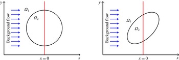
The first example is Stokes flow around a circular or elliptical porous region in the presence of a uniform constant background flow. The schematic plot of the problem is shown in figure 2 for two different cases. The figure illustrates the background flow from left to right and a vertical line where the velocity profile will be computed. Since
 $\unicode[STIX]{x1D6FA}_{1}$
is a Stokes flow region, we set
 $(\unicode[STIX]{x1D6FC}_{1},\unicode[STIX]{x1D719}_{1})=(0,1)$
. We impose the jump conditions in (3.42)–(3.44), which are the Ochoa-Tapia–Whitaker (OTW) conditions in this case.
Schematic plot of the problem where a porous region described by the Brinkman equations is surrounded by a viscous fluid. The regions in the examples in this section are either circular or elliptical. The background flow is uniformly constant and equal to
 $\boldsymbol{u}^{\infty }=(20,0)^{t}$
. The velocity profiles will be shown across the vertical lines.

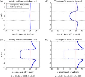
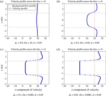
Figure 3 shows the velocity profiles across the vertical line
 $x=0$
, for different values of
 $(\unicode[STIX]{x1D6FC}_{2},\unicode[STIX]{x1D719}_{2})$
. Note that the interval
 $y\in (-1,1)$
corresponds to the region inside the circle. Figure 3(a) shows a case with porosity
 $\unicode[STIX]{x1D719}_{2}=0.9$
so that the porous medium region is 90 % fluid, resulting in a very small disturbance relative to the background flow. Figure 3(b–d) shows the velocity profiles for decreasing values of
 $\unicode[STIX]{x1D719}_{2}$
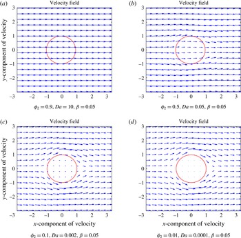
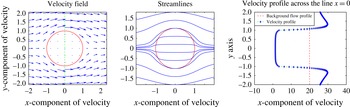
. For the circular region in figure 3(d), where the porous medium is nearly solid and the resistance to the external flow is high, the velocity inside the circle is negligible. Figure 4 shows the flow through and around the porous region.
Velocity profiles: effects of porosity on the velocity field in a domain with circular interface. Continuity of the velocity and the normal stress along with ‘OTW’ jump condition on the tangential stress are imposed at the interface. On the vertical axes,
 $\unicode[STIX]{x1D6FA}_{2}$
corresponds to
 $-1\leqslant y\leqslant 1$
. The parameter
 $\unicode[STIX]{x1D6FC}$
is defined by
 $\unicode[STIX]{x1D6FC}=\sqrt{\unicode[STIX]{x1D719}/Da}$
.

Velocity fields for various values of porosity
 $\unicode[STIX]{x1D719}$
and
 $Da$
. The parameter
 $\unicode[STIX]{x1D6FC}$
is defined by
 $\unicode[STIX]{x1D6FC}=\sqrt{\unicode[STIX]{x1D719}/Da}$
.

Results for an elliptical interface rotated
 $45^{\circ }$
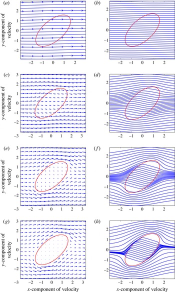
with respect to the background flow are shown in figures 5 and 6. As the parameter values change, similar behaviour as the circular case can be seen in the velocity profiles, i.e. they also show more resistance to the flow inside the ellipse as porosity and permeability decreases. The velocity field and associated streamlines are shown in figure 6. The streamlines inside the porous ellipse evolve as
 $\unicode[STIX]{x1D719}\rightarrow 0$
. The flow when
 $\unicode[STIX]{x1D719}_{2}=0.9$
is approximately undisturbed; as
 $\unicode[STIX]{x1D719}_{2}$
decreases, the outer flow tends to penetrate less the porous medium and go around it. The orientation of the ellipse causes the streamlines inside the porous region to tilt relative to the background flow. Similar streamline patterns have been observed and discussed before for the case of flow around and through a porous sphere (Bhattacharyya Reference Bhattacharyya2010).
A
 $45^{\circ }$
rotated elliptical interface: velocity profiles associated with different values of the porosity and the permeability across the line
 $x=0$
are plotted. On the vertical axes,
 $\unicode[STIX]{x1D6FA}_{2}$
corresponds to
 $-1.265\leqslant y\leqslant 1.265$
. The parameter
 $\unicode[STIX]{x1D6FC}$
is defined by
 $\unicode[STIX]{x1D6FC}=\sqrt{\unicode[STIX]{x1D719}/Da}$
.

Velocity fields are shown in (a,c,e,g) and their corresponding streamlines in (b,d,f,h). The parameter
 $\unicode[STIX]{x1D6FC}$
is defined by
 $\unicode[STIX]{x1D6FC}=\sqrt{\unicode[STIX]{x1D719}/Da}$
. (a,b)
 $\unicode[STIX]{x1D719}_{2}=0.9$
,
 $Da=10$
,
 $\unicode[STIX]{x1D6FD}=0.05$
, (c,d)
 $\unicode[STIX]{x1D719}_{2}=0.5$
,
 $Da=0.05$
,
 $\unicode[STIX]{x1D6FD}=0.05$
, (e,f)
 $\unicode[STIX]{x1D719}_{2}=0.1$
,
 $Da=0.002$
,
 $\unicode[STIX]{x1D6FD}=0.05$
, (g,h)
 $\unicode[STIX]{x1D719}_{2}=0.01$
,
 $Da=0.0001$
,
 $\unicode[STIX]{x1D6FD}=0.05$
.

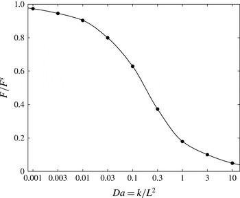
We also compute the variation of the force on the stationary porous disc in a viscous fluid moving with constant speed as a function of Darcy number (dimensionless permeability). The force is scaled by the drag magnitude on a solid disc,
 $F^{s}=8\unicode[STIX]{x03C0}\unicode[STIX]{x1D707}U^{\infty }/(2a\ln (a)-a)$
, with
 $a=1$
. We set
 $\boldsymbol{f}^{(1)}$
and
 $\boldsymbol{f}^{(2)}$
is related to the interface fluid velocity through the stress interface jump condition. The force on the porous disc is the integral of
 $\boldsymbol{f}^{(2)}$
over the disc surface. The value of
 $\unicode[STIX]{x1D6FD}$
was set as in (1.12) with
 $\unicode[STIX]{x1D6FE}=0.002/(1-\unicode[STIX]{x1D719})^{2/3}$
(Valdés-Parada et al.
Reference Valdés-Parada, Goyeau and Ochoa-Tapia2007). The results are shown in figure 7. The values of the porosity are chosen independently and the results are sensitive to those values. Here the values were increasing from
 $\unicode[STIX]{x1D719}=0.1105$
for the smallest value of
 $Da$
to
 $\unicode[STIX]{x1D719}=0.99$
for the largest
 $Da$
. The results are similar to corresponding ones in three dimensions by Higdon & Kojima (Reference Higdon and Kojima1981).
Hydrodynamic force on a porous disc as a function of dimensionless permeability.

4.2 Brinkman–Brinkman problem
In this section we illustrate the results of our model for the general case of a Brinkman medium with parameters
 $(\unicode[STIX]{x1D6FC}_{1},\unicode[STIX]{x1D719}_{1})$
surrounding a different Brinkman medium with parameters
 $(\unicode[STIX]{x1D6FC}_{2},\unicode[STIX]{x1D719}_{2})$
. The fluid is assumed to have viscosity
 $\unicode[STIX]{x1D707}$
and there is a uniform background flow from left to right. We use (3.23)–(3.25) and compute the velocity field associated with the flow around and through a circular porous disc.
We first investigate the effect of the jump coefficient
 $\unicode[STIX]{x1D6FD}$
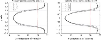
in the tangential stress condition (3.44). Figure 8 shows the horizontal velocity profile along a vertical line through the centre of the disc when the parameters are
 $(\unicode[STIX]{x1D6FC}_{1},\unicode[STIX]{x1D719}_{1})=(2.45,0.6)$
and
 $(\unicode[STIX]{x1D6FC}_{2},\unicode[STIX]{x1D719}_{2})=(2.83,0.4)$
. As before, the fluid velocity at the interface is first computed with (3.25) and the velocities in domains
 $\unicode[STIX]{x1D6FA}_{1}$
and
 $\unicode[STIX]{x1D6FA}_{2}$
are then computed using (3.23)–(3.24). The interface conditions in (3.42)–(3.44) are used. Figure 8 shows a comparison between the flows when
 $\unicode[STIX]{x1D6FD}$
ranges from
 $-2$
to
 $2$
, including the value
 $\unicode[STIX]{x1D6FD}=0$
(continuity of all stresses). The velocity profiles on the left side of figure 8 show that as
 $\unicode[STIX]{x1D6FD}$
becomes more negative, the velocity profile inside the disc exhibits less variation compared to the
 $\unicode[STIX]{x1D6FD}=0$
case. On the other hand, when
 $\unicode[STIX]{x1D6FD}>0$
the velocity profiles inside the disc develop larger gradients as
 $\unicode[STIX]{x1D6FD}$
increases. These results point to the sensitivity of the velocity field to the jump coefficient
 $\unicode[STIX]{x1D6FD}$
and the importance of imposing appropriate values based on the physical problem under consideration.
Horizontal velocity profiles corresponding to a circular porous region
 $\unicode[STIX]{x1D6FA}_{2}$
surrounded by a different porous region
 $\unicode[STIX]{x1D6FA}_{1}$
. The parameters used are
 $\unicode[STIX]{x1D719}_{1}=0.6$
,
 $\unicode[STIX]{x1D6FC}_{1}=2.45$
and
 $\unicode[STIX]{x1D719}_{2}=0.4$
,
 $\unicode[STIX]{x1D6FC}_{2}=2.83$
. The panels show the profiles obtained by using different values of the jump coefficient
 $\unicode[STIX]{x1D6FD}$
.

Figures 9 and 10 show the velocity field, its corresponding streamlines and the velocity profile across the vertical line
 $x=0$
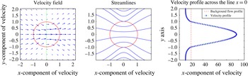
for different parameter values. In figure 9 the porosity of the circular disc is smaller than the exterior region so that the flow experiences a sufficiently high resistance within the disc that much of the fluid goes around the disc. Figure 9 can be compared with figure 3(d), where the flow parameters inside the disc are the same but they differ outside. In the latter, the outer region contains a Stokes flow so the exterior flow is faster in general while inside it is slightly slower. Also the general shape of the velocity profile is smoother when the point crosses the interface in Brinkman–Brinkman flow compared to the Stokes–Brinkman flow. A final example shows the case of two porous media where the inner circular region has higher porosity (less resistance), see figure 10. In this case the flow in the disc is faster than in the exterior, which was observed by Yano, Kieda & Mizuno (Reference Yano, Kieda and Mizuno1991) in the case of a viscous droplet surrounded by a porous medium in two dimensions.
Brinkman–Brinkman system with
 $(\unicode[STIX]{x1D6FC}_{1},\unicode[STIX]{x1D719}_{1})=(3.16,0.2)$
,
 $(\unicode[STIX]{x1D6FC}_{2},\unicode[STIX]{x1D719}_{2})=(10,0.01)$
and
 $\unicode[STIX]{x1D6FD}=0.4$
.

Brinkman–Brinkman system with
 $(\unicode[STIX]{x1D6FC}_{1},\unicode[STIX]{x1D719}_{1})=(3.16,0.2)$
,
 $(\unicode[STIX]{x1D6FC}_{2},\unicode[STIX]{x1D719}_{2})=(0.85,0.8)$
and
 $\unicode[STIX]{x1D6FD}=0.9$
.

5 Conclusion
We have presented a boundary integral formulation for the flow in a domain where a porous medium is surrounded by another porous medium of different permeability, which had not been presented before. Previous work had focused on a porous particle within a viscous environment described by the Stokes equations. We used the Brinkman equation coupled with the incompressibility of the fluid to model the flow in the porous media. The derivation of the boundary integral formulation relies on the continuity of the velocity across the interface between the two media and on the jump in the double layer potential in (3.29), which we showed to be equal to the jump in the Stokes–Stokes case. The formulation includes the effect of a uniform background flow.
The Brinkman–Brinkman integral formulation depends on
 $f_{i}^{(1)}=\unicode[STIX]{x1D70E}_{ik}^{(1)}n_{k}$
and
 $f_{i}^{(2)}=\unicode[STIX]{x1D70E}_{ik}^{(2)}n_{k}$
in a way that cannot be written simply as a function of the difference between the surface traction on either side of the interface,
 $\unicode[STIX]{x0394}f_{i}=f_{i}^{(1)}-f_{i}^{(2)}$
as in the case of a droplet in Stokes flow. Moreover, the double layer potential on the left side of (3.29) depends on the evaluation point
 $\boldsymbol{x}_{0}$
and the dimensionless parameter
 $\unicode[STIX]{x1D6FC}$
of each region in such a way that the jump is the same at every point of the interface.
When the surface tractions are not known independently, additional relations between surface tractions are needed. These relations depend on the microscopic quantities of the porous media and on the specific characteristics of the interface in the physical problem under consideration (Pozrikidis Reference Pozrikidis1992). Using the Ochoa-Tapia–Whitaker jump condition for a porous medium in a Stokes flow as a guide, a general jump condition for the tangential stresses was derived for the Brinkman–Brinkman case. The condition has the properties that the jump vanishes when the properties of the two media are equal and that it reduces to the Ochoa-Tapia–Whitaker jump condition when the permeability of the outside medium is infinite. As part of the formulation, the stress jump coefficient can also be set to zero to enforce continuity of stress.
Examples were presented to illustrate the effect of the interface conditions in two-dimensional flows. As discussed in the Introduction, the choice of jump coefficient
 $\unicode[STIX]{x1D6FD}$
remains under investigation. In the case of two porous media with a common closed interface, figure 8 shows differences in the first component of velocity for different values of
 $\unicode[STIX]{x1D6FD}$
. The panels illustrate that the flow is sensitive to this parameter and that a reasonably accurate value of
 $\unicode[STIX]{x1D6FD}$
is required in simulations. For specific applications, such as flow through bacterial biofilms (Cogan, Cortez & Fauci Reference Cogan, Cortez and Fauci2005; Klapper & Dockery Reference Klapper and Dockery2010), we expect the parameter
 $\unicode[STIX]{x1D6FD}$
to be chosen based on experimental data.
Acknowledgement
This work was funded in part by National Science Foundation grant DMS-1217223.
Appendix A
We consider an incompressible Brinkman flow due to a single point force
 $\boldsymbol{g}$
located at
 $\boldsymbol{x}_{0}$
in a domain,
 $\unicode[STIX]{x1D6FA}$
, bounded by a closed smooth surface, denoted by
 $\unicode[STIX]{x2202}\unicode[STIX]{x1D6FA}$
. Then the flow in this domain is described by
 $$\begin{eqnarray}\displaystyle & \displaystyle \unicode[STIX]{x1D6FC}^{2}\frac{\unicode[STIX]{x1D702}}{\unicode[STIX]{x1D719}}\boldsymbol{u}=-\unicode[STIX]{x1D735}p+\frac{\unicode[STIX]{x1D702}}{\unicode[STIX]{x1D719}}\unicode[STIX]{x0394}\boldsymbol{u}+\boldsymbol{g}\unicode[STIX]{x1D6FF}(\boldsymbol{x}-\boldsymbol{x}_{0}), & \displaystyle\end{eqnarray}$$
 $$\begin{eqnarray}\displaystyle & \displaystyle \unicode[STIX]{x1D735}\boldsymbol{\cdot }\boldsymbol{u}=0. & \displaystyle\end{eqnarray}$$
We will use the notation
 $$\begin{eqnarray}\displaystyle & \displaystyle u_{i}(\boldsymbol{x}_{0})=\frac{\unicode[STIX]{x1D719}}{\unicode[STIX]{x1D702}}\unicode[STIX]{x1D61A}_{ij}(\boldsymbol{x},\boldsymbol{x}_{0};\unicode[STIX]{x1D6FC})g_{j}, & \displaystyle\end{eqnarray}$$
 $$\begin{eqnarray}\displaystyle & \displaystyle p=P_{j}(\boldsymbol{x},\boldsymbol{x}_{0})g_{j}, & \displaystyle\end{eqnarray}$$
 $$\begin{eqnarray}\displaystyle & \displaystyle \unicode[STIX]{x1D70E}_{ik}=\unicode[STIX]{x1D61B}_{ijk}(\boldsymbol{x},\boldsymbol{x}_{0})g_{j}=-P_{j}g_{j}\unicode[STIX]{x1D6FF}_{ik}+\left[\frac{\unicode[STIX]{x2202}\unicode[STIX]{x1D61A}_{ij}}{\unicode[STIX]{x2202}x_{k}}+\frac{\unicode[STIX]{x2202}S_{kj}}{\unicode[STIX]{x2202}x_{i}}\right]g_{j} & \displaystyle\end{eqnarray}$$
for the velocity, pressure and stress tensor. Note that
 $\unicode[STIX]{x1D61B}_{ijk}=\unicode[STIX]{x1D61B}_{kji}$
.
Then, the Brinkman equation (A 1) can be expressed as
 $$\begin{eqnarray}\unicode[STIX]{x1D6FC}^{2}\unicode[STIX]{x1D61A}_{ij}(\boldsymbol{x},\boldsymbol{x}_{0})=-\frac{\unicode[STIX]{x2202}P_{j}}{\unicode[STIX]{x2202}x_{i}}+\unicode[STIX]{x0394}\unicode[STIX]{x1D61A}_{ij}(\boldsymbol{x},\boldsymbol{x}_{0};\unicode[STIX]{x1D6FC})+\unicode[STIX]{x1D6FF}_{ij}\unicode[STIX]{x1D6FF}(\boldsymbol{x}-\boldsymbol{x}_{0}),\end{eqnarray}$$
where
 $\unicode[STIX]{x1D6FF}_{ij}$
is the Kronecker delta and
 $\unicode[STIX]{x1D6FF}(\boldsymbol{x})$
is the Dirac delta function. On the other hand,
 $$\begin{eqnarray}\frac{\unicode[STIX]{x2202}\unicode[STIX]{x1D61B}_{ijk}}{\unicode[STIX]{x2202}x_{k}}=-\frac{\unicode[STIX]{x2202}P_{j}}{\unicode[STIX]{x2202}x_{k}}\unicode[STIX]{x1D6FF}_{ik}+\left[\frac{\unicode[STIX]{x2202}^{2}\unicode[STIX]{x1D61A}_{ij}}{\unicode[STIX]{x2202}x_{k}\unicode[STIX]{x2202}x_{k}}+\frac{\unicode[STIX]{x2202}^{2}S_{kj}}{\unicode[STIX]{x2202}x_{k}\unicode[STIX]{x2202}x_{i}}\right]=-\frac{\unicode[STIX]{x2202}P_{j}}{\unicode[STIX]{x2202}x_{i}}+\frac{\unicode[STIX]{x2202}^{2}\unicode[STIX]{x1D61A}_{ij}}{\unicode[STIX]{x2202}x_{k}\unicode[STIX]{x2202}x_{k}},\end{eqnarray}$$
where the last equality in (A 7) follows from the incompressibility condition (A 2). Plugging (A 6) into (A 7) we obtain
 $$\begin{eqnarray}\displaystyle \frac{\unicode[STIX]{x2202}\unicode[STIX]{x1D61B}_{ijk}}{\unicode[STIX]{x2202}x_{k}}=\unicode[STIX]{x1D6FC}^{2}\unicode[STIX]{x1D61A}_{ij}(\boldsymbol{x},\boldsymbol{x}_{0};\unicode[STIX]{x1D6FC})-\unicode[STIX]{x1D6FF}_{ij}\unicode[STIX]{x1D6FF}(\boldsymbol{x}-\boldsymbol{x}_{0}). & & \displaystyle\end{eqnarray}$$
Integrating this last equation over the domain
 $\unicode[STIX]{x1D6FA}$
and using the divergence theorem we obtain
 $$\begin{eqnarray}\displaystyle \int _{\unicode[STIX]{x2202}\unicode[STIX]{x1D6FA}}\unicode[STIX]{x1D61B}_{ijk}(\boldsymbol{x},\boldsymbol{x}_{0};\unicode[STIX]{x1D6FC})n_{k}(\boldsymbol{x})\,\text{d}S & = & \displaystyle \int _{\unicode[STIX]{x2202}\unicode[STIX]{x1D6FA}}\unicode[STIX]{x1D61B}_{kji}(\boldsymbol{x},\boldsymbol{x}_{0};\unicode[STIX]{x1D6FC})n_{k}(\boldsymbol{x})\,\text{d}S\nonumber\\ \displaystyle & = & \displaystyle \unicode[STIX]{x1D6FC}^{2}\int _{\unicode[STIX]{x1D6FA}}\unicode[STIX]{x1D61A}_{ij}(\boldsymbol{x},\boldsymbol{x}_{0};\unicode[STIX]{x1D6FC})\,\text{d}\boldsymbol{x}-{\mathcal{A}}\unicode[STIX]{x1D6FF}_{ij},\end{eqnarray}$$
where for a smooth boundary
 $$\begin{eqnarray}{\mathcal{A}}=\left\{\begin{array}{@{}ll@{}}1\quad & \text{if }\boldsymbol{x}_{0}\in \unicode[STIX]{x1D6FA}\\ 1/2\quad & \text{if }\boldsymbol{x}_{0}\in \unicode[STIX]{x2202}\unicode[STIX]{x1D6FA}\\ 0\quad & \text{if }\boldsymbol{x}_{0}\notin \unicode[STIX]{x1D6FA}.\end{array}\right.\end{eqnarray}$$
Note that if
 $\unicode[STIX]{x1D6FC}\rightarrow 0$
, equation (A 9) reduces to the known jump in the double layer potential for Stokes flows (Pozrikidis Reference Pozrikidis1992).
Appendix B
We consider a closed porous–porous interface where a constant background flow was present in the porous medium 1 region,
 $\unicode[STIX]{x1D6FA}_{1}$
. The fluid velocity and pressure in the domain
 $\unicode[STIX]{x1D6FA}_{1}$
,
 $\boldsymbol{u}^{(1)}$
and
 $p^{(1)}$
, satisfy
 $$\begin{eqnarray}\unicode[STIX]{x1D735}\boldsymbol{\cdot }\boldsymbol{u}^{(1)}=0,\quad \frac{\unicode[STIX]{x1D6FC}_{1}^{2}}{\unicode[STIX]{x1D719}_{1}}\boldsymbol{u}^{(1)}=-\unicode[STIX]{x1D735}p^{(1)}+\frac{1}{\unicode[STIX]{x1D719}_{1}}\unicode[STIX]{x0394}\boldsymbol{u}^{(1)}.\end{eqnarray}$$
In the domain
 $\unicode[STIX]{x1D6FA}_{2}$
,
 $\boldsymbol{u}^{(2)}$
and
 $p^{(2)}$
satisfy
 $$\begin{eqnarray}\unicode[STIX]{x1D735}\boldsymbol{\cdot }\boldsymbol{u}^{(2)}=0,\quad \frac{\unicode[STIX]{x1D702}_{2}\unicode[STIX]{x1D6FC}_{2}^{2}}{\unicode[STIX]{x1D719}_{2}}\boldsymbol{u}^{(2)}=-\unicode[STIX]{x1D735}p^{(2)}+\frac{\unicode[STIX]{x1D702}_{2}}{\unicode[STIX]{x1D719}_{2}}\unicode[STIX]{x0394}\boldsymbol{u}^{(2)},\end{eqnarray}$$
where
 $\unicode[STIX]{x1D702}_{2}=\unicode[STIX]{x1D707}_{2}/\unicode[STIX]{x1D707}_{1}$
. Consider a constant background flow
 $\boldsymbol{u}^{\infty }$
in
 $\unicode[STIX]{x1D6FA}_{1}$
, then
 $$\begin{eqnarray}\unicode[STIX]{x1D735}\boldsymbol{\cdot }\boldsymbol{u}^{\infty }=0,\quad \frac{\unicode[STIX]{x1D6FC}_{1}^{2}}{\unicode[STIX]{x1D719}_{1}}\boldsymbol{u}^{\infty }=-\unicode[STIX]{x1D735}p^{\infty }.\end{eqnarray}$$
The boundary conditions are
 $\boldsymbol{u}^{(1)}=\boldsymbol{u}^{(2)}$
at the interface and
 $\boldsymbol{u}^{(1)}\rightarrow \boldsymbol{u}^{\infty }$
as
 $r\rightarrow \infty$
.
Next we define the disturbance flows
 $\tilde{\boldsymbol{u}}^{(1)}=\boldsymbol{u}^{(1)}-\boldsymbol{u}^{\infty }$
,
 $\tilde{p}^{(1)}=p^{(1)}-p^{\infty }$
,
 $\tilde{\boldsymbol{u}}^{(2)}=\boldsymbol{u}^{(2)}-c\boldsymbol{u}^{\infty }$
and
 $\tilde{p}^{(2)}=p^{(2)}-p^{\infty }$
, where
 $c=(\unicode[STIX]{x1D719}_{2}\unicode[STIX]{x1D6FC}_{1}^{2})/(\unicode[STIX]{x1D719}_{1}\unicode[STIX]{x1D702}_{2}\unicode[STIX]{x1D6FC}_{2}^{2})$
. With these definitions, the disturbance velocities satisfy
 $$\begin{eqnarray}\unicode[STIX]{x1D735}\boldsymbol{\cdot }\tilde{\boldsymbol{u}}^{(1)}=0,\quad \frac{\unicode[STIX]{x1D6FC}_{1}^{2}}{\unicode[STIX]{x1D719}_{1}}\tilde{\boldsymbol{u}}^{(1)}=-\unicode[STIX]{x1D735}\tilde{p}^{(1)}+\frac{1}{\unicode[STIX]{x1D719}_{1}}\unicode[STIX]{x0394}\tilde{\boldsymbol{u}}^{(1)}\end{eqnarray}$$
and
 $$\begin{eqnarray}\unicode[STIX]{x1D735}\boldsymbol{\cdot }\tilde{\boldsymbol{u}}^{(2)}=0,\quad \frac{\unicode[STIX]{x1D702}_{2}\unicode[STIX]{x1D6FC}_{2}^{2}}{\unicode[STIX]{x1D719}_{2}}\tilde{\boldsymbol{u}}^{(2)}=-\unicode[STIX]{x1D735}\tilde{p}^{(2)}+\frac{\unicode[STIX]{x1D702}_{2}}{\unicode[STIX]{x1D719}_{2}}\unicode[STIX]{x0394}\tilde{\boldsymbol{u}}^{(2)}.\end{eqnarray}$$
The continuity of the fluid velocity implies that the disturbance velocities satisfy
 $\tilde{\boldsymbol{u}}^{(1)}+\boldsymbol{u}^{\infty }=\tilde{\boldsymbol{u}}^{(2)}+c\boldsymbol{u}^{\infty }$
and
 $\tilde{\boldsymbol{u}}^{(1)}\rightarrow 0$
as
 $r\rightarrow \infty$
. Also, the stress tensors are
 $$\begin{eqnarray}\displaystyle & \displaystyle \tilde{\unicode[STIX]{x1D70E}}_{ik}^{(1)}=-(p^{(1)}-p^{\infty })\unicode[STIX]{x1D6FF}_{ik}+\frac{1}{\unicode[STIX]{x1D719}_{1}}\left(\frac{\unicode[STIX]{x2202}u_{i}^{(1)}}{\unicode[STIX]{x2202}x_{k}}+\frac{\unicode[STIX]{x2202}u_{k}^{(1)}}{\unicode[STIX]{x2202}x_{i}}\right), & \displaystyle\end{eqnarray}$$
 $$\begin{eqnarray}\displaystyle & \displaystyle \tilde{\unicode[STIX]{x1D70E}}_{ik}^{(2)}=-(p^{(2)}-p^{\infty })\unicode[STIX]{x1D6FF}_{ik}+\frac{\unicode[STIX]{x1D702}_{2}}{\unicode[STIX]{x1D719}_{2}}\left(\frac{\unicode[STIX]{x2202}u_{i}^{(2)}}{\unicode[STIX]{x2202}x_{k}}+\frac{\unicode[STIX]{x2202}u_{k}^{(2)}}{\unicode[STIX]{x2202}x_{i}}\right), & \displaystyle\end{eqnarray}$$
which implies that
 $\tilde{f}_{i}^{(1)}=f_{i}^{(1)}+p^{\infty }n_{i}$
and
 $\tilde{f}_{i}^{(2)}=f_{i}^{(2)}+p^{\infty }n_{i}$
.
Let
 $\boldsymbol{x}_{0}\in \unicode[STIX]{x1D6FA}_{1}$
, then use (3.14) and (3.15) to obtain
 $$\begin{eqnarray}\displaystyle \tilde{u} _{j}^{(1)}(\boldsymbol{x}_{0}) & = & \displaystyle -\unicode[STIX]{x1D719}_{1}\int _{\unicode[STIX]{x2202}\unicode[STIX]{x1D6FA}}\unicode[STIX]{x1D61A}_{ij}(\boldsymbol{x},\boldsymbol{x}_{0};\unicode[STIX]{x1D6FC}_{1})[f_{i}^{(1)}+p^{\infty }n_{i}]\,\text{d}\ell (\boldsymbol{x})\nonumber\\ \displaystyle & & \displaystyle +\,\int _{\unicode[STIX]{x2202}\unicode[STIX]{x1D6FA}}\tilde{u} _{i}^{(1)}(\boldsymbol{x})\unicode[STIX]{x1D61B}_{ijk}(\boldsymbol{x},\boldsymbol{x}_{0};\unicode[STIX]{x1D6FC}_{1})n_{k}(\boldsymbol{x})\,\text{d}\ell (\boldsymbol{x}),\end{eqnarray}$$
and
 $$\begin{eqnarray}0=\frac{\unicode[STIX]{x1D719}_{2}}{\unicode[STIX]{x1D702}_{2}}\int _{\unicode[STIX]{x2202}\unicode[STIX]{x1D6FA}}\unicode[STIX]{x1D61A}_{ij}(\boldsymbol{x},\boldsymbol{x}_{0};\unicode[STIX]{x1D6FC}_{2})[f_{i}^{(2)}+p^{\infty }n_{i}]\,\text{d}\ell (\boldsymbol{x})-\int _{\unicode[STIX]{x2202}\unicode[STIX]{x1D6FA}}\tilde{u} _{i}^{(2)}(\boldsymbol{x})\unicode[STIX]{x1D61B}_{ijk}(\boldsymbol{x},\boldsymbol{x}_{0};\unicode[STIX]{x1D6FC}_{2})n_{k}(\boldsymbol{x})\,\text{d}\ell (\boldsymbol{x}).\end{eqnarray}$$
Therefore, adding (B 8)
 $+$
 $\unicode[STIX]{x1D719}_{1}\unicode[STIX]{x1D702}_{2}/\unicode[STIX]{x1D719}_{2}$
(B 9) eliminates
 $p^{\infty }$
and gives
 $$\begin{eqnarray}\displaystyle \tilde{u} _{j}^{(1)}(\boldsymbol{x}_{0}) & = & \displaystyle -\unicode[STIX]{x1D719}_{1}\int _{\unicode[STIX]{x2202}\unicode[STIX]{x1D6FA}}[\unicode[STIX]{x1D61A}_{ij}(\boldsymbol{x},\boldsymbol{x}_{0};\unicode[STIX]{x1D6FC}_{1})f_{i}^{(1)}-\unicode[STIX]{x1D61A}_{ij}(\boldsymbol{x},\boldsymbol{x}_{0};\unicode[STIX]{x1D6FC}_{2})f_{i}^{(2)}]\,\text{d}\ell (\boldsymbol{x})\nonumber\\ \displaystyle & & \displaystyle +\,\int _{\unicode[STIX]{x2202}\unicode[STIX]{x1D6FA}}\left[\tilde{u} _{i}^{(1)}\unicode[STIX]{x1D61B}_{ijk}(\boldsymbol{x},\boldsymbol{x}_{0};\unicode[STIX]{x1D6FC}_{1})-\frac{\unicode[STIX]{x1D719}_{1}\unicode[STIX]{x1D702}_{2}}{\unicode[STIX]{x1D719}_{2}}\tilde{u} _{i}^{(2)}\unicode[STIX]{x1D61B}_{ijk}(\boldsymbol{x},\boldsymbol{x}_{0};\unicode[STIX]{x1D6FC}_{2})\right]n_{k}(\boldsymbol{x})\,\text{d}\ell (\boldsymbol{x}).\qquad\end{eqnarray}$$
Since
 $\tilde{\boldsymbol{u}}^{(1)}=\boldsymbol{u}^{(1)}-\boldsymbol{u}^{\infty }$
and
 $\tilde{\boldsymbol{u}}^{(2)}=\boldsymbol{u}^{(2)}-(\unicode[STIX]{x1D719}_{2}\unicode[STIX]{x1D6FC}_{1}^{2}/\unicode[STIX]{x1D719}_{1}\unicode[STIX]{x1D702}_{2}\unicode[STIX]{x1D6FC}_{2}^{2})\boldsymbol{u}^{\infty }$
, or equivalently
 $(\unicode[STIX]{x1D719}_{1}\unicode[STIX]{x1D702}_{2}/\unicode[STIX]{x1D719}_{2})\tilde{\boldsymbol{u}}^{(2)}=(\unicode[STIX]{x1D719}_{1}\unicode[STIX]{x1D702}_{2}/\unicode[STIX]{x1D719}_{2})\boldsymbol{u}^{(2)}-(\unicode[STIX]{x1D6FC}_{1}/\unicode[STIX]{x1D6FC}_{2})^{2}\boldsymbol{u}^{\infty }$
, equation (B 10) can be expressed as
 $$\begin{eqnarray}\displaystyle u_{j}^{(1)}(\boldsymbol{x}_{0}) & = & \displaystyle u_{j}^{\infty }(\boldsymbol{x}_{0})-\int _{\unicode[STIX]{x2202}\unicode[STIX]{x1D6FA}}u_{i}^{\infty }(\boldsymbol{x})\left[\unicode[STIX]{x1D61B}_{ijk}(\boldsymbol{x},\boldsymbol{x}_{0};\unicode[STIX]{x1D6FC}_{1})-\frac{\unicode[STIX]{x1D6FC}_{1}^{2}}{\unicode[STIX]{x1D6FC}_{2}^{2}}\unicode[STIX]{x1D61B}_{ijk}(\boldsymbol{x},\boldsymbol{x}_{0};\unicode[STIX]{x1D6FC}_{2})\right]n_{k}(\boldsymbol{x})\,\text{d}\ell (\boldsymbol{x})\nonumber\\ \displaystyle & & \displaystyle -\,\unicode[STIX]{x1D719}_{1}\int _{\unicode[STIX]{x2202}\unicode[STIX]{x1D6FA}}[\unicode[STIX]{x1D61A}_{ij}(\boldsymbol{x},\boldsymbol{x}_{0};\unicode[STIX]{x1D6FC}_{1})f_{i}^{(1)}-\unicode[STIX]{x1D61A}_{ij}(\boldsymbol{x},\boldsymbol{x}_{0};\unicode[STIX]{x1D6FC}_{2})f_{i}^{(2)}]\,\text{d}\ell (\boldsymbol{x})\nonumber\\ \displaystyle & & \displaystyle +\,\int _{\unicode[STIX]{x2202}\unicode[STIX]{x1D6FA}}u_{i}(\boldsymbol{x})[\unicode[STIX]{x1D61B}_{ijk}(\boldsymbol{x},\boldsymbol{x}_{0};\unicode[STIX]{x1D6FC}_{1})-\unicode[STIX]{x1D706}\unicode[STIX]{x1D61B}_{ijk}(\boldsymbol{x},\boldsymbol{x}_{0};\unicode[STIX]{x1D6FC}_{2})]n_{k}(\boldsymbol{x})\;\text{d}\ell (\boldsymbol{x}),\end{eqnarray}$$
where
 $\unicode[STIX]{x1D706}=\unicode[STIX]{x1D719}_{1}\unicode[STIX]{x1D702}_{2}/\unicode[STIX]{x1D719}_{2}$
. Equation (B 11) is the boundary integral representation of the flow in the domain
 $\unicode[STIX]{x1D6FA}_{1}$
, in the presence of a constant background flow.
Using a similar calculation when
 $\boldsymbol{x}_{0}\in \unicode[STIX]{x1D6FA}_{2}$
, we arrive at
 $$\begin{eqnarray}\displaystyle u_{j}^{(2)}(\boldsymbol{x}_{0}) & = & \displaystyle \frac{1}{\unicode[STIX]{x1D706}}\left(\frac{\unicode[STIX]{x1D6FC}_{1}^{2}}{\unicode[STIX]{x1D6FC}_{2}^{2}}u_{j}^{\infty }-u_{i}^{\infty }\int _{\unicode[STIX]{x2202}\unicode[STIX]{x1D6FA}}\left[\unicode[STIX]{x1D61B}_{ijk}(\boldsymbol{x},\boldsymbol{x}_{0};\unicode[STIX]{x1D6FC}_{1})-\frac{\unicode[STIX]{x1D6FC}_{1}^{2}}{\unicode[STIX]{x1D6FC}_{2}^{2}}\unicode[STIX]{x1D61B}_{ijk}(\boldsymbol{x},\boldsymbol{x}_{0};\unicode[STIX]{x1D6FC}_{2})\right]n_{k}(\boldsymbol{x})\,\text{d}\ell (\boldsymbol{x})\right.\nonumber\\ \displaystyle & & \displaystyle -\,\frac{\unicode[STIX]{x1D719}_{1}}{\unicode[STIX]{x1D702}_{1}}\int _{\unicode[STIX]{x2202}\unicode[STIX]{x1D6FA}}[\unicode[STIX]{x1D61A}_{ij}(\boldsymbol{x},\boldsymbol{x}_{0};\unicode[STIX]{x1D6FC}_{1})f_{i}^{(1)}-\unicode[STIX]{x1D61A}_{ij}(\boldsymbol{x},\boldsymbol{x}_{0};\unicode[STIX]{x1D6FC}_{2})f_{i}^{(2)}]\,\text{d}\ell (\boldsymbol{x})\nonumber\\ \displaystyle & & \displaystyle +\left.\int _{\unicode[STIX]{x2202}\unicode[STIX]{x1D6FA}}u_{i}(\boldsymbol{x})[\unicode[STIX]{x1D61B}_{ijk}(\boldsymbol{x},\boldsymbol{x}_{0};\unicode[STIX]{x1D6FC}_{1})-\unicode[STIX]{x1D706}\unicode[STIX]{x1D61B}_{ijk}(\boldsymbol{x},\boldsymbol{x}_{0};\unicode[STIX]{x1D6FC}_{2})]n_{k}(\boldsymbol{x})\,\text{d}\ell (\boldsymbol{x})\right),\end{eqnarray}$$
which is the boundary integral representation of the flow in the domain
 $\unicode[STIX]{x1D6FA}_{2}$
, in presence of a constant background flow
 $\boldsymbol{u}^{\infty }$
.
Next, in (B 11) and (B 12), let
 $\boldsymbol{x}_{0}\rightarrow \unicode[STIX]{x2202}\unicode[STIX]{x1D6FA}$
from both sides of the interface to obtain
 $$\begin{eqnarray}\displaystyle u_{j}(\boldsymbol{x}_{0}) & = & \displaystyle \frac{1}{2}\left[1+\frac{\unicode[STIX]{x1D6FC}_{1}^{2}}{\unicode[STIX]{x1D6FC}_{2}^{2}}\right]u_{j}^{\infty }-\int _{\unicode[STIX]{x2202}\unicode[STIX]{x1D6FA}}^{\,pv}u_{i}^{\infty }\left[\unicode[STIX]{x1D61B}_{ijk}(\boldsymbol{x},\boldsymbol{x}_{0};\unicode[STIX]{x1D6FC}_{1})-\frac{\unicode[STIX]{x1D6FC}_{1}^{2}}{\unicode[STIX]{x1D6FC}_{2}^{2}}\unicode[STIX]{x1D61B}_{ijk}(\boldsymbol{x},\boldsymbol{x}_{0};\unicode[STIX]{x1D6FC}_{2})\right]n_{k}(\boldsymbol{x})\,\text{d}\ell (\boldsymbol{x})\nonumber\\ \displaystyle & & \displaystyle -\,\unicode[STIX]{x1D719}_{1}\int _{\unicode[STIX]{x2202}\unicode[STIX]{x1D6FA}}[\unicode[STIX]{x1D61A}_{ij}(\boldsymbol{x},\boldsymbol{x}_{0};\unicode[STIX]{x1D6FC}_{1})f_{i}^{(1)}-\unicode[STIX]{x1D61A}_{ij}(\boldsymbol{x},\boldsymbol{x}_{0};\unicode[STIX]{x1D6FC}_{2})f_{i}^{(2)}]\,\text{d}\ell (\boldsymbol{x})\nonumber\\ \displaystyle & & \displaystyle +\,\int _{\unicode[STIX]{x2202}\unicode[STIX]{x1D6FA}}^{\,pv}u_{i}(\boldsymbol{x})[\unicode[STIX]{x1D61B}_{ijk}(\boldsymbol{x},\boldsymbol{x}_{0};\unicode[STIX]{x1D6FC}_{1})-\unicode[STIX]{x1D706}\unicode[STIX]{x1D61B}_{ijk}(\boldsymbol{x},\boldsymbol{x}_{0};\unicode[STIX]{x1D6FC}_{2})]n_{k}(\boldsymbol{x})\,\text{d}\ell (\boldsymbol{x})\nonumber\\ \displaystyle & & \displaystyle +\,\frac{1}{2}(1-\unicode[STIX]{x1D706})u_{j}(\boldsymbol{x}_{0}),\end{eqnarray}$$
and
 $$\begin{eqnarray}\displaystyle u_{j}(\boldsymbol{x}_{0}) & = & \displaystyle \frac{1}{\unicode[STIX]{x1D706}}\left(\frac{1}{2}\left[1+\frac{\unicode[STIX]{x1D6FC}_{1}^{2}}{\unicode[STIX]{x1D6FC}_{2}^{2}}\right]u_{j}^{\infty }-\!\int _{\unicode[STIX]{x2202}\unicode[STIX]{x1D6FA}}^{\,pv}u_{i}^{\infty }\left[\unicode[STIX]{x1D61B}_{ijk}(\boldsymbol{x},\boldsymbol{x}_{0};\unicode[STIX]{x1D6FC}_{1})-\frac{\unicode[STIX]{x1D6FC}_{1}^{2}}{\unicode[STIX]{x1D6FC}_{2}^{2}}\unicode[STIX]{x1D61B}_{ijk}(\boldsymbol{x},\boldsymbol{x}_{0};\unicode[STIX]{x1D6FC}_{2})\right]\!n_{k}(\boldsymbol{x})\,\text{d}\ell (\boldsymbol{x})\right.\nonumber\\ \displaystyle & & \displaystyle -\,\unicode[STIX]{x1D719}_{1}\int _{\unicode[STIX]{x2202}\unicode[STIX]{x1D6FA}}[\unicode[STIX]{x1D61A}_{ij}(\boldsymbol{x},\boldsymbol{x}_{0};\unicode[STIX]{x1D6FC}_{1})f_{i}^{(1)}-\unicode[STIX]{x1D61A}_{ij}(\boldsymbol{x},\boldsymbol{x}_{0};\unicode[STIX]{x1D6FC}_{2})f_{i}^{(2)}]\,\text{d}\ell (\boldsymbol{x})\nonumber\\ \displaystyle & & \displaystyle +\,\int _{\unicode[STIX]{x2202}\unicode[STIX]{x1D6FA}}u_{i}(\boldsymbol{x})[\unicode[STIX]{x1D61B}_{ijk}(\boldsymbol{x},\boldsymbol{x}_{0};\unicode[STIX]{x1D6FC}_{1})-\unicode[STIX]{x1D706}\unicode[STIX]{x1D61B}_{ijk}(\boldsymbol{x},\boldsymbol{x}_{0};\unicode[STIX]{x1D6FC}_{2})]n_{k}(\boldsymbol{x})\,\text{d}\ell (\boldsymbol{x})\nonumber\\ \displaystyle & & \displaystyle -\left.\frac{1}{2}(1-\unicode[STIX]{x1D706})u_{j}(\boldsymbol{x}_{0})\right).\end{eqnarray}$$
Then (B 13)
 $+$
 $\unicode[STIX]{x1D706}$
(B 14) gives us
 $$\begin{eqnarray}\displaystyle u_{j}(\boldsymbol{x}_{0}) & = & \displaystyle \frac{2}{1+\unicode[STIX]{x1D706}}\left(\frac{1}{2}\left[1+\frac{\unicode[STIX]{x1D6FC}_{1}^{2}}{\unicode[STIX]{x1D6FC}_{2}^{2}}\right]u_{j}^{\infty }\right.\nonumber\\ \displaystyle & & \displaystyle -\,u_{i}^{\infty }\int _{\unicode[STIX]{x2202}\unicode[STIX]{x1D6FA}}^{\,pv}\left[\unicode[STIX]{x1D61B}_{ijk}(\boldsymbol{x},\boldsymbol{x}_{0};\unicode[STIX]{x1D6FC}_{1})-\frac{\unicode[STIX]{x1D6FC}_{1}^{2}}{\unicode[STIX]{x1D6FC}_{2}^{2}}\unicode[STIX]{x1D61B}_{ijk}(\boldsymbol{x},\boldsymbol{x}_{0};\unicode[STIX]{x1D6FC}_{2})\right]n_{k}(\boldsymbol{x})\,\text{d}\ell (\boldsymbol{x})\nonumber\\ \displaystyle & & \displaystyle -\,\unicode[STIX]{x1D719}_{1}\int _{\unicode[STIX]{x2202}\unicode[STIX]{x1D6FA}}[\unicode[STIX]{x1D61A}_{ij}(\boldsymbol{x},\boldsymbol{x}_{0};\unicode[STIX]{x1D6FC}_{1})f_{i}^{(1)}-\unicode[STIX]{x1D61A}_{ij}(\boldsymbol{x},\boldsymbol{x}_{0};\unicode[STIX]{x1D6FC}_{2})f_{i}^{(2)}]\,\text{d}\ell (\boldsymbol{x})\nonumber\\ \displaystyle & & \displaystyle +\left.\int _{\unicode[STIX]{x2202}\unicode[STIX]{x1D6FA}}^{\,pv}u_{i}(\boldsymbol{x})[\unicode[STIX]{x1D61B}_{ijk}(\boldsymbol{x},\boldsymbol{x}_{0};\unicode[STIX]{x1D6FC}_{1})-\unicode[STIX]{x1D706}\unicode[STIX]{x1D61B}_{ijk}(\boldsymbol{x},\boldsymbol{x}_{0};\unicode[STIX]{x1D6FC}_{2})]n_{k}(\boldsymbol{x})\,\text{d}\ell (\boldsymbol{x})\right),\end{eqnarray}$$
which is the boundary integral representation of the flow at the interface, in the presence of a constant background flow
 $\boldsymbol{u}^{\infty }$
.