1 Introduction
The automatisation of text data analysis in insurance is a promising and challenging field, due to the importance of reports and analysis in the treatment of claims or contracts. In this paper, we focus on data coming from expert reports on a claim, but textual informations may be found also in declarations filled by policyholders themselves, or in medical questionaries used in credit insurance. Our aim is to process these reports and develop an automatic way to categorise the corresponding claims and to identify, soon after their occurrence, which one will lead to a heavy loss. Apart from the complexity of the input information, a particular difficulty is caused by the rareness of such claims (a few percent of the total database).
The rise of deep learning techniques introduces the possibility of developing an automated treatment of these data, with potential reduced costs – and, ideally, a more accurate analysis – for the insurance company, hence a potential increase of rentability. Text mining has received a lot of attention in the past decades in the machine learning literature, with many spectacular examples. Many examples can be found, for example, in Aggarwal & Zhai (Reference Aggarwal and Zhai2012) or Berry & Castellanos (Reference Berry and Castellanos2004), with applications to insurance such as Ellingsworth & Sullivan (Reference Ellingsworth and Sullivan2003) or Kolyshkina & van Rooyen (Reference Kolyshkina and van Rooyen2006).
As we already mentioned, our main difficulty is to focus on the prediction of relatively rare events, which is a classical specificity of the insurance business compared to other fields. Indeed, while typical claims and behaviour are usually easy to understand and measure, the tail of the distribution of the losses is much more delicate, since there are quite few events in the database to evaluate it properly. Of course, these so-called “extreme” events may, in some cases, constitute an important part of the total losses at a portfolio level.
In this paper, we consider the case of text data coming from experts in view of clustering some claims depending on their severity. Typically, the insurance company wants to separate “benign” claims from the heaviest ones in order to perform a different treatment of these two types of claims. Indeed, in terms of reserving, a different model can be used on these two types of events. Moreover, a particular attention can then be devoted to the most serious claims during their development. As described above, the difficulty is that the proportion of heavy claims is quite low compared to the other class. This imbalance is present in other potential applications, such as fraud detection. We rely on deep neural networks methodologies. Neural networks have already demonstrated to be valuable tools when it comes to evaluating claims, see, for example, Saputro et al. (Reference Saputro, Murfi and Nurrohmah2019) or Wüthrich (Reference Wüthrich2018). The network architectures that we use – Convolutional Neural Networks (CNNs), see Aloysius & Geetha (Reference Aloysius and Geetha2017), and Recurrent Neural Networks (RNNs) (such as Long Short-Term Memory (LSTM) networks introduced by Hochreiter & Schmidhuber (Reference Hochreiter and Schmidhuber1997)) – are powerful tools to perform such text analysis, see, for example, Mikolov et al. (Reference Mikolov, Karafiát, Burget, Černocky and Khudanpur2010) and Cheng et al. (Reference Cheng, Dong and Lapata2016). The specificity of our approach is twofold:
We introduce a bias correction in order to deal with the fact that claim development time may be long: indeed, our models are calibrated on a database made of claims that are closed, but also from unsettled ones. Calibrating the model on the closed claims solely would introduce some bias due to the over-representation of claims with small development time (this is a classical problem linked to the concept of censoring in survival analysis, see, for example, Lopez, Reference Lopez2019; Gerber et al., Reference Gerber, Faou, Lopez and Trupin2020).
Once this bias correction has been done, a re-equilibration of the database is required to compensate the rareness of the events we focus on. For this, we use Bagging methodologies (for Bootstrap Aggregating, see Breiman, Reference Breiman1996), introducing constraints in the resampling methodology which is at the core of Bagging.
The contribution of this paper is to show how performing these two tasks (censoring correction and re-equilibration) can improve existing deep learning methods to analyse a corpus of texts which is very specific: indeed, apart from the rareness of the event that are considered, the reports on car insurance claims that we study in our applications, are characterised by a very specific vocabulary and a particular syntax that makes text classification more challenging.
The rest of the paper is organised as follows. In section 2, we describe the general framework and the general methodology to address these two points. A particular focus on processing text data is shown in section 3, where we explain the process of embedding such data (this means to perform an adapted dimension reduction to represent efficiently such complex unstructured data). The deep neural networks architectures that we use are then described in section 4. In section 5, a real example on a database coming from a French insurer gives indications on the performance of the methodology.
2 Framework and Neural Network Predictors
In this section, we describe the generic structure of our data. Our data are subject to random censoring, as a time variable (time of settlements of the claims) is present in the database. The correction of this phenomenon, via classical methodologies from survival analysis, is described in section 2.1. Next, the general framework of neural networks is defined in section 2.2. The imbalance in the data, caused by the fact that we focus on predicting rare events, is described in section 2.3, along with methodologies to improve the performance of our machine learning approaches under this constraint.
2.1 The censoring framework
Our aim is to predict a 0–1 random response I, which depends on a time variable T and covariates  $\textbf{X}\in \mathcal{X}\subset \mathbb{R}^d.$ In our practical application, I is an indicator of the severity of a claim (
 $I=1$ if the claim is considered as “extreme”, 0 otherwise). The definition of what we refer to as an extreme claim depends on management conventions that will be described in the real data section. The variable T represents the total length of the claim (i.e. the time between the claim occurence and its final settlement), and
 $\textbf{X}$ some characteristics.
In our setting, the variables I and T are not observed directly. Since T is a duration variable, it is subject to right censoring. This means that, for the claims that are still not settled, T is unknown. On the other hand, I is known only if the claim is closed. This leads to the following observations  $(J_i, Y_i, \delta_i, \textbf{X}_i)_{1\leq i \leq n}$ assumed to be i.i.d. replications of
 $(J,Y,\delta,\textbf{X})$ where
 \begin{equation*}\left\{\begin{array}{c@{\hspace*{2pt}}c@{\hspace*{2pt}}l} Y &=& \inf(T,C), \\[4pt]\delta&=& \textbf{1}_{T\leq C}, \\[5pt]J &=& \delta I\end{array}\right.\end{equation*}
and  $\textbf{X}$ represents some covariates that are fully observed (in our case,
 $\textbf{X}$ is text data coming from reports, hence it can be understood as a vector in
 $\mathbb{R}^{d}$ with d being huge: more precisely,
 $\textbf{X}$ can be understood as a matrix, each column representing an appropriate coding of a word, see section 3, the number of columns being the total number of words). The variable C is called the censoring variable and is assumed to be random. The censoring variable corresponds to the time after which the claim stops to be observed for any other reason than its settlement (either because the observation period ends before settlement, or because there has been a retrocession of the claim). This setting is similar to the one developed by Lopez et al. (Reference Lopez, Milhaud and Thérond2016) or Lopez (Reference Lopez2019) in the case of claim reserving, with a variable I that may not be binary in the general case. In the following, we assume that T and C have continuous distributions so that these variables are perfectly symmetric, which means that one has the same level of information on the distribution of T as on the distribution of T (otherwise, a dissymmetry can appear due to ties, since one could have
 $\mathbb{P}(T=C)\neq 0,$ leading to potential inconsistencies, see Stute & Wang, Reference Stute and Wang1993).
Considering only the complete data (i.e. with  $\delta_i=1,$ which corresponds to the case where the claim is settled) would introduce some bias: amongst the complete of observations, there is an overrepresentation of claims associated with a small value of
 $T_i.$ Since T and I are dependent (in practice, one often observes a positive correlation between T and the corresponding amount of the claim), neglecting censoring would imbalance the sample, modifying the proportion of values of i for which
 $I_i=1.$
Our aim is to estimate the function  $\pi(\textbf{x})=\mathbb{P}(I=1|\textbf{X}=\textbf{x}),$ in a context where the dimension d of
 $\textbf{x}$ is large. Typically, how an estimated function fits data is quantified by minimising some loss function. If we were dealing with complete data, a natural choice would be the logistic loss function (also called “cross entropy” in the neural network literature, see, for example, Kline & Berardi, Reference Kline and Berardi2005), that is
 \begin{equation*}L^*_n(p)=-\frac{1}{n}\sum_{i=1}^n \left\{I_i \log p +(1-I_i)\log(1-p)\right\}\end{equation*}
which is a consistent estimator of
 \begin{equation*}L(p)=-E\left[I \log p+(1-I)\log (1-p)\right]\end{equation*}
As stated before, computation of  $L_n^*$ is impossible in presence of censoring due to the lack of information, and an adaptation is required to determine a consistent estimator of L.
A simple way to correct the bias caused by censoring is to rely on the Inverse Probability of Censoring Weighting (IPCW) strategy, see, for example, Rotnitzky & Robins (Reference Rotnitzky and Robins2014). The idea of this approach is to find a function  $y\rightarrow W(y)$ such that, for all positive function
 $\psi$ with finite expectation,
 \begin{align}E \left[ \delta W(Y)\psi (J,Y,\textbf{X})\right]=E \left[ \psi (I,T,\textbf{X})\right]\end{align}
and to try to estimate this function W (in full generality, this function can also depend on  $\textbf{X}$). The function W depends on the identifiability assumptions that are required to be able to retrieve the distribution of I and T from the data. In the following, we assume that
1. C is independent from (J,T)
2.
 $\mathbb{P}(T\leq C | I,T,\textbf{X})=\mathbb{P}(T\leq C | T),$

as in Lopez (Reference Lopez2019), and is similar to the one used, for example, in Stute (Reference Stute1996) or Stute (Reference Stute1999) in a censored regression framework. These two conditions ensure that (1) holds to  $W(y)=S_C(y)^{-1}=\mathbb{P}(C\geq y)^{-1},$ provided that
 $\inf\{t:S_C(t)=0\}\geq \inf\{t:\mathbb{P}(T\geq t)=0\},$ which will be assumed throughout this paper. These assumptions are identifiability assumptions that can not be tested statistically, see Andersen et al. (Reference Andersen, Borgan, Gill and Keiding1998), section III.2.2.3 p. 148. Alternative assumptions can be found, for example, in Van Keilegom & Akritas (Reference Van Keilegom and Akritas1999), and the procedure we develop can be modified to address this more complex situation, in the same spirit as Gerber et al. (Reference Gerber, Faou, Lopez and Trupin2020). In the real data application that we consider in section 5 below, censoring is mainly caused by administrative issues (the claim is not closed at the date of extraction of the database), which makes these more classical identifiability assumptions reasonable. This also ensures that W is strictly positive and finite.
 $S_C$ can then be consistently estimated by the Kaplan–Meier estimator (see Kaplan & Meier, Reference Kaplan and Meier1958), that is
 \begin{equation*}\hat{S}_C(t)=\prod_{Y_i\leq t} \left(1- \frac{\delta_i}{\sum_{j=1}^n\mathds{1}_{Y_j\geq Y_i}}\right)\end{equation*}
Consistency of Kaplan–Meier estimator has been derived by Stute (Reference Stute1995) and Akritas et al. (Reference Akritas2000).
Hence, each quantity of the type  $E \left[ \psi (I,T,\textbf{X})\right]$ can be estimated by
 $\sum_{i=1}^n W_{i,n}\psi(J_i,Y_i,\textbf{X}_i)$ where
 \begin{equation}W_{i,n}=\delta_in^{-1}\hat{S}_C(Y_i)^{-1}\end{equation}
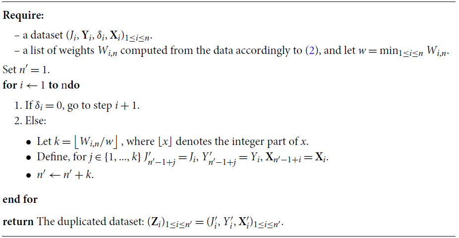
In other words, a way to correct the bias caused by the censoring consists in attributing the weight  $W_{i,n}$ at observation i. This weight is 0 for censored observations, and the missing mass is attributed to complete observations with an appropriate rule. A convenient way to apply this weight once and for all is to duplicate the complete observations in the original data accordingly to their weight. This is a way to artificially (but consistently) compensate the lack of complete observations associated with a large value of
 $Y_i$ (let us observe that
 $W_{i,n}$ is an increasing function of
 $Y_i$). This leads to the following duplication algorithm.
Duplication algorithm for censored observations

The cross-entropy that we want to minimise is then computed from the duplicated dataset, defining
 \begin{equation}L_{n^{\prime}}(p)=-\frac{1}{n^{\prime}}\sum_{i=1}^{n^{\prime}} \left\{J^{\prime}_i \log p +(1-J^{\prime}_i)\log (1-p)\right\}\end{equation}
Remark. In the experimental part of the paper, we will also introduce two alternative loss functions, which can be seen as modifications of cross-entropy. The focal-loss (see Lin et al., Reference Lin, Goyal, Girshick, He and Dollár2017) is defined as
 \begin{equation}\tilde{L}_{n^{\prime}}(p)=-\frac{1}{n^{\prime}}\sum_{i=1}^{n^{\prime}} \left\{{J^{\prime}}_{i^{\gamma}} \log p +(1-J^{\prime}_i)^\gamma\log (1-p)\right\}\end{equation}
where  $\gamma \geq 0.$ The parameter
 $\gamma$ helps to focus on “hard” examples, by avoiding attributing too much weights at easily well-predicted observations. The Weighted Cross-Entropy (see Panchapagesan et al., Reference Panchapagesan, Sun, Khare, Matsoukas, Mandal, Hoffmeister and Vitaladevuni2016) is a weighted version of (3). Introducing a weight
 $\alpha\in (0,1),$ define
 \begin{equation}\bar{L}_{n^{\prime}}(p)=-\frac{1}{n^{\prime}}\sum_{i=1}^{n^{\prime}} \left\{J^{\prime}_i \alpha \log p +(1-\alpha)(1-J^{\prime}_i)\log (1-p)\right\}\end{equation}
The parameter  $\alpha$ can be used to increase the importance of good prediction for one of the two classes, or to reflect its under-representation in the sample.
2.2 Neural network under censoring
A neural network (see, for example, Hastie et al., Reference Hastie, Tibshirani and Friedman2009, Chapter 11) is an over-parametrised function  $\textbf{x}\rightarrow p(\textbf{x},\theta),$ that we will use in the following to estimate function
 $\pi.$ By over-parametrised, we mean that
 $\theta \in \mathbb{R}^k,$ with k usually much larger than d (the dimension of
 $\textbf{x}$). The function
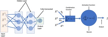
 $p(\cdot,\theta)$ can also have a complex structure depending on the architecture of the network, that we present in more details in section 4. Typically, a neural network is a function that can be represented as shown in Figure 1. Following the notations of Figure 1, each neuron is described by a vector of weights
 $\textbf{w}$ (of the same size as
 $\textbf{x}$), a bias term b (one-dimensional), and an activation function f used to introduce some non-linearity. Typical choices of functions f are described in Table A.1. Following our notations,
 $\theta$ represents the list of the weights and bias parameters corresponding to all neurons of the network. For a given value of
 $\theta$ and an input
 $\textbf{x},$ the computation of
 $p(\textbf{x},\theta)$ is usually called “forward propagation”.
Left-hand side: representation of a simple neural network (multilayer perceptron). Each unit of the network (represented by a circle), is called a neuron (a neuron is represented on the right-hand side).  $X^{(j)}$ represents the jth component of the covariate vector
 $\textbf{X}.$

On the other hand, “backward propagation” (see Rumelhart et al., Reference Rumelhart, Hinton and Williams1986) is the algorithmic procedure used to optimise the value of the parameter  $\theta.$ Since our aim is to estimate the function
 $\pi,$ fitting the neural network consists of trying to determine
 \begin{equation*}\theta^*=\arg \min_{\theta} L_{n^{\prime}}(p(\cdot,\theta))\end{equation*}
where we recall that  $L_n$ has been defined in equation (3) (or, alternatively, using
 $\tilde{L}_{n^{\prime}}$ or
 $\bar{L}_{n^{\prime}}$ from (4) and (5)), and is adapted to the presence of censoring since computed on the duplicated dataset obtained from Algorithm 1.
2.3 Bagging for imbalanced data
Bagging (for bootstrap aggregating, see Breiman, Reference Breiman1996) is a classical way to stabilise machine learning algorithms. The heuristic behind bagging is to avoid overfitting, and to perform a synthesis (through the aggregation of results) of different calibrations of the models, which stabilises the results. In an ideal situation, one would use aggregation of models calibrated on totally different datasets generated from the same distribution as the one we are targeting through our statistical analysis. This is of course impossible, since generating the observed random sample is an experiment that can not be replicated indefinitely, so pseudo samples are generated by bootstrap, using the empirical distribution of the data instead of the true (unknown) one. Instead, bootstrap resampling is used to create pseudo samples. In our case, a different neural network is fitted from each pseudo sample, before aggregating all the results. Introducing bootstrap is expected to reduce the variance of estimation, while avoiding overfitting.
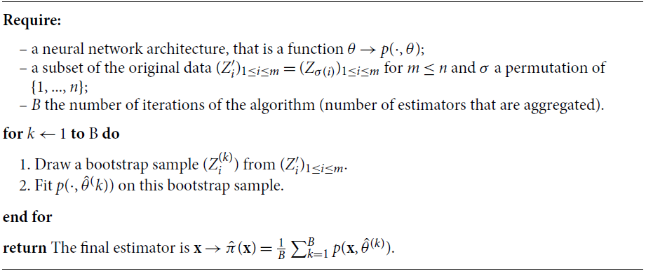
Formally, the procedure can be described in the following way.
Bagging algorithm applied to neural networks

A particular difficulty in applying bagging to our classification problem is that we have a problem in which a class is under-represented amongst our observations. If we were to apply bagging as in Algorithm 2 directly, many bootstrap samples may contain too few observations from the smallest class to produce an accurate prediction. This could limit considerably the performance of the resulting estimator.
For structured data, methods like SMOTE (see Chawla et al., Reference Chawla, Bowyer, Hall and Kegelmeyer2002) can be used to generate new observations to enrich the database. Data augmentation techniques are also available for image analysis, see Ronneberger et al. (Reference Ronneberger, Fischer and Brox2015). These techniques are difficult to adapt to our text analysis framework, since they implicitly rely on the assumption that there is some spatial structure underlying data: typically, if the observations are represented as points in a multi-dimensional space, SMOTE joins two points associated with label 1, and introduce a new pseudo observation somewhere on a segment joining them. In our situation, labels are scattered through this high-dimensional space, and the procedure does not seem adapted.
We here propose two simple ways to perform rebalancing, that we refer to as “Balanced bagging” and “Randomly balanced bagging” respectively.
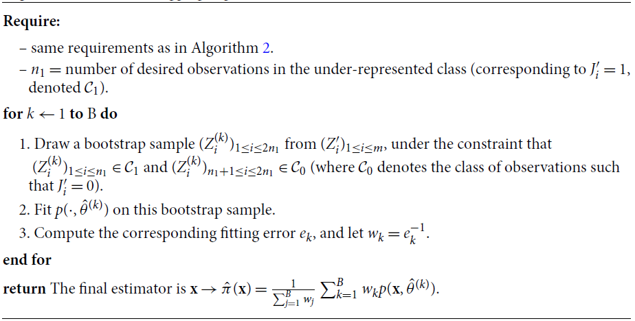
Balanced bagging:
Balanced Bagging Algorithm

Randomly balanced bagging:
Randomly Balanced Bagging Algorithm

In each case, the final aggregated estimator perform the synthesis of each step, giving more importance to step k if its fitting error  $e_k$ is small.
2.4 Summary of our methodology
Let us summarise our methodology, which combines bias correction (censoring correction), and bagging strategies to compute our predictor. First, we compute Kaplan–Meier weights and use them to duplicate data according to these weights as described in Algorithm 1. Then, from a given neural network architecture, we use one of the bagging algorithms of section 2.3 to create pseudo samples, and aggregate the fitted networks to obtain our final estimator  $\hat{\pi}(\textbf{x}).$
The quality of the prediction strongly depends on two aspects that have still not been mentioned in this general description of the method:
Pre-processing of text data: this step consists in finding the proper representation of the words contained in the reports in a continuous space, adapted to defining a proper distance between words.
Architecture: the performance is strongly dependent on the type of neural networks used (number of layers, structure of the cells and connexions).
This two points are developed in sections 3 and 4, respectively.
3 Embedding Methodology
In this section, we discuss the particularity of dealing with text data. To be analysed by neural networks structures, text data first require to be transformed into covariates of large dimension in an appropriate space. After discussing one-hot encoding in section 3.1, we will explain the concept of word embedding in section 3.2. A combination of the standard Fasttext embedding methodology (see Joulin et al., Reference Joulin, Grave, Bojanowski, Douze, Jégou and Mikolov2016a) with our database of text reports is discussed in section 3.2.1.
3.1 One-hot encoding
Since our procedure aims at automatically treating text data and use them to predict the severity of a claim, we need to find a convenient representation of texts so that it can be treated efficiently by our network. The first idea is to rely on one-hot encoding. The set of whole words in the reports forms a dictionary of size V (Vocabulary size), then each word is associated to a number  $1\leq j \leq V.$ A report is then represented as a matrix. If there is l words in the report, we encode it as a matrix
 $\textbf{X}=(x_{a,b})_{1\leq a \leq V, 1\leq b \leq l},$ with V lines and l columns. The kth column represents the kth word of the report, say
 $\textbf{x}_{k}$. If this word is the jth word of the dictionary, then
 $x_{j,k}=1$ and
 $x_{i,k}=0$ for all
 $i\neq j.$ Hence, each column has exactly one non-zero value.
To introduce some context of use of the words, the size of the dictionary can be increased by not considering single words but n-grams. A n-gram is a contiguous sequence of n items from a given sample of text or speech (either a sequence of words, or of letters). The vocabulary size V becomes the total number of n-grams contained in the report.
Using one-hot encoding makes the data ready for machine learning treatment, but it raises at least two difficulties:
− the vocabulary size V is huge.
− It is not adapted to defining a convenient distance between words. Indeed, we want to take into account that there are similarities between words (synonyms, for instance, or even spelling errors).
Hence, there is a need for a more compact representation that would define a proper metric on words.
3.2 Word embedding
This process of compacting the information is called word embedding, see Bojanowski et al. (Reference Bojanowski, Grave, Joulin and Mikolov2016), Joulin et al. (Reference Joulin, Grave, Bojanowski and Mikolov2016b). The idea of embedding is to map each column of a one-hot encoded matrix to a lower dimension vector (whose components are real numbers, not only 0–1 valued).
Embedding consists in defining dense vector representations of the characters. The objectives of these projections are:
− Dimension Reduction: as already mentioned, embedding maps a sparse vector of size V to a lower dense vector of size
$N < V$.− Semantic Similarity: typically, words that are similar or that are often associated, will be close in terms of embedded vectors.

To perform embedding, we will use a linear transform of vectors. This transformation is defined by the embedding matrix W (V columns and N lines). A one-hot encoded report  $\textbf{X}$ is then transformed into
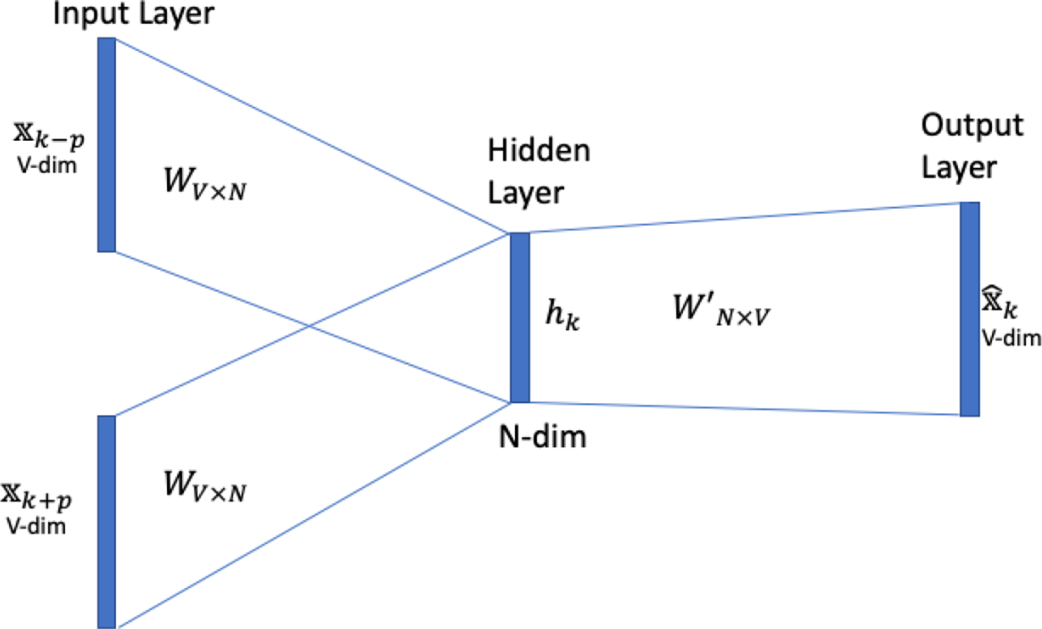
 $\textbf{X}^{\prime}=W\textbf{X}$ (according to the notations of section 2), which becomes the input of our neural network models. How to determine a proper matrix W is described by the diagram of Figure 2. A full description of the steps of the methodology is the following:
a “context window” of size
$c=2p+1$ is centred on the current word $\textbf{x}_k$: this defines a set of c words $(\textbf{x}_{k-j})_{-p \leq j \leq p}$ that are used as inputs of the procedure of Figure 2.The embedding matrix W is applied to each of these words, and an hidden layer, producing, for the kth group of words,
$h_k=C^{-1}\sum_{j=-p}^p W \textbf{x}_k.$The N-dimensional vector
$h_k$ is then sent back to the original V-dimensional space by computing ${\hat{\textbf{x}}}_k=W^{\prime}h_k=(\hat{x}_{j,k})_{1\leq j \leq V},$ where $W’$ denotes the synaptic matrix of the hidden layer also called the “context embedding”.


Summary of the embedding matrix determination.

The error used to measure the quality of the embedding for word k is
 \begin{equation*}-\sum_{j=1}^V \log \left(\frac{\exp\!(x_{j,k}\hat{x}_{j,k})}{\sum_{l=1}^V\exp\!(x_{l,k}\hat{x}_{l,k})}\right)\end{equation*}
A global error is then obtained by summing all the words of the report, and by summing over all the reports. The embedding matrix is the one which minimises this criterion. In this paper, we consider embedding through neural networks, but alternative methodologies such as Pennington et al. (Reference Pennington, Socher and Manning2014) can be used.
3.2.1 FastText
The gist of FastText, see Joulin et al. (Reference Joulin, Grave, Bojanowski, Douze, Jégou and Mikolov2016a), is that instead of directly learning a vector representation for a word (as with Word2vec, see Mikolov et al., Reference Mikolov, Sutskever, Chen, Corrado and Dean2013; Rong, Reference Rong2014), the words are decomposed into small character n-grams (see Bojanowski et al., Reference Bojanowski, Grave, Joulin and Mikolov2017), and one learns a representation for each n-gram. A word is represented as words being represented as the sum of these representations. So even if a word is misspelled, its representation tends to be close to the one of the well-spelled words. Moreover, FastText proposes an efficient algorithm to optimise the choice of the embedding matrix. A pre-trained FastText embedding matrix is available, trained on a huge number of words. Nevertheless, it has not been calibrated from on a vocabulary and a context specific to insurance. Hence, a possibility that we develop in the following is to use the FastText algorithm (not the pre-trained matrix), but training our embedding matrix on the corpus of insurance reports from our database.
In the following, we distinguish between three ways of performing embedding:
the matrix W is determined via FastText’s algorithm once and for all at the beginning of the procedure. The embedded words are sent as inputs into the network architectures described in the following section 4. Only the parameters of these networks are iteratively optimised. We call this method “static” embedding.
The embedding is considered as a first (linear) layer of the network. The values of the embedding matrix W are initialised with FastText’s algorithm, but updated at the same time the other coefficients of the network are optimised. We call this method “non-static”.
For comparison, we also consider the case of a random initialisation of this matrix W, whose coefficients are then updated in the same way as in the non-static method. We refer to it as the “random” method.
4 Network Architectures for Text Data
The architecture of neural networks is a key element that can considerably impact their performance. We consider to types of architectures in the following:
CNNs, described in section 4.1;
LSTM networks which are a particular kind of RNNs, described in section 4.2.
4.1 Convolutional Neural Network
CNNs are nowadays widely used for image processing (image clustering, segmentation, object detection…), see, for example, Krizhevsky et al. (Reference Krizhevsky, Sutskever and Hinton2012). Kim (Reference Kim2014) showed that they can achieve nice performance on text analysis. Compared to the multilayer perceptron, which is the most simple class of neural network and corresponds to the architecture described in Figure 1, CNN are based on a particular spatial structure that prevents overfitting.
A CNN is made of different type of layers composing the network. One may distinguish between:
convolutional layers: each neuron only focus on a localised part of the input, see below;
fully connected layers: every neuron of the layer is connected to every neuron in the following one;
normalisation layers: used to normalise the inputs coming from the previous layer;
padding and pooling layers: the aim is either to expand or to reduce the dimension of the inputs coming from the previous layer through simple operations, see below;
the final output layer that produces a prediction of the label through combination of the results of the previous layer.
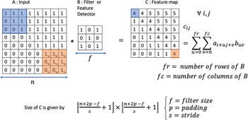
The convolutional layers are at the core of the idea of spatial structure of CNNs. They extract features from the input while preserving the spatial relationship between the coordinates of the embedding matrix. Typically, they operate simple combinations of coefficients whose coordinates are closed to each other, as illustrated in Figure 3.
An example of a convolution layer. Convolution Layer. Each coefficient  $c_{i,j}$ of the output matrix is obtained by a linear combinations of coefficients
 $a_{i,j}$ in a
 $f\times f$ square of the input matrix. The colour code shows which coefficients of the input matrix have been used to compute the corresponding coefficient of C.

In CNN terminology, the matrix B in Figure 3 is called a “filter” (sometimes “kernel” or “feature detector”) and the matrix formed by sliding the filter over the input and computing the dot product is called the “Convolved Feature” (“Activation Map” or “Feature Map”). A filter slides over the input (denoted by A in Figure 3) to produce a feature map. Each coefficient of the output matrix (C in Figure 3) is made of a linear combination of the coefficients of A is a small square of the input matrix. This linear combination is a convolution operation. Each convolution layer aims to capture local dependencies in the original input. Moreover, different filters make appear different features, that is different structures in the input data. In practice, a CNN learns the values of these filters on its own during the training process (although we still need to specify parameters such as number of filters, filter size, architecture of the network before the training process). The higher the number of filters, the more features get extracted, increasing the ability of the network to recognise patterns in unseen inputs.
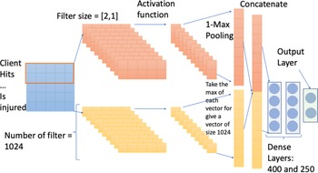
The other types of layers are described in section 7.2. An example of CNN architecture is described in the real data application, see Figure 7.
4.2 Recurrent Neural Networks and Long Short-Term Memory (LSTM) networks
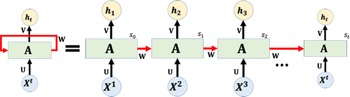
RNN are designed to handle dependent inputs. This is the case when dealing with text, since a change in the order of words induce a change of meaning of a sentence. Therefore, where conventional neural networks consider that input and output data are independent, RNNs consider an information sequence. A representation of a RNN is provided in Figure 4.
A unrolled RNN and the unfolding representation in time of the computation involved in its forward computation.

According to this diagram, the different (embedded) words (or n-grams) constituting a report, pass successively into the network A. The t-h network produces an output (the final one constituting the prediction), but also a memory cell  $c_t$ which is sent to the next block. Hence, each single network uses a regular input (that is an embedded word), plus the information coming from the memory cell. This memory cell is the way to keep track on previous information. The most simple way to keep this information would be to identify the memory cell with the output of each network. Hence, the t-th network uses the information from the past in the sense that it take advantage of the prediction done at the previous step. Nevertheless, this could lead to a fade of the contribution of the first words of the report, while they could be determinant.
To circumvent this issue, one can turn at LSTM networks have been introduced by Hochreiter & Schmidhuber (Reference Hochreiter and Schmidhuber1997). They can be considered as a particular class of RNN with a design which allows to keep track of the information in a more flexible way. The purpose of LSTM is indeed to introduce a properly designed memory cell whose content evolves with t to keep relevant information through time (and “forget” irrelevant).
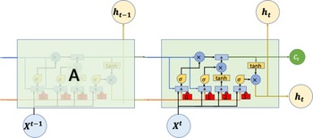
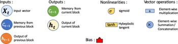
As RNN, LSTM are successive blocks of networks. Each block can be described by Figure 5 (whose notations are summarized in Figure 6). The specificity of LSTM is the presence of a “cell”  $c_t$ which differs from the output
 $h_t, $ and which can be understood as a channel to convey context information that may be relevant to compute the following output
 $h_{t+1}$ in the next block of the network. The information contained in the cell passes through three gates. These so-called gates are simple operations that permit to keep, add or remove information to the memory cell.
Synthetic description of a block of a LSTM network.

LSTM notations.

Following the diagram of Figure 5, the memory cell  $c_t$ first goes through a multiplicative gate. This mean that each component of the vector
 $c_t$ is multiplied by a number between 0 and 1 (contained in a vector
 $f_t$), which allows to keep (value close to 1) or suppress (value close to 0) the information contained in each component of
 $c_t.$ This vector
 $f_t$ is computed from the new input
 $x_t$ and the output of the previous block
 $h_{t-1}.$
Next, the modified memory cell enters an additive gate. This gate is used to add information. The added information is a vector  $\tilde{C}_t,$ again computed from the input
 $x_t$ and the previous output
 $h_{t-1}.$ This produces the updated memory cell that passes through the next block.
Moreover, this memory cell is transformed and combined with  $(x_t,h_{t-1})$ through the third step, to produce a new output.
To summarise, the following set of operations are performed in each unit (here,  $\sigma$ denotes the classical sigmoid function, and
 $[x_t,h_{t-1}]$ the concatenation of the vectors
 $x_t$ and
 $h_t$):
Compute
$u_t=\sigma(\theta_0 [x_t,h_{t-1}]+b_0),$ $v_t=\sigma(\theta_1[x_t,h_{t-1}]+b_1),$ and $w_t=\tanh(\theta_2[x_t,\break h_{t-1}]+b_2).$The updated value of the memory cell is
$c_t=u_t\times c_{t-1}+v_t\times w_t.$The new output is
$h_t=\sigma(\theta_3 [x_t,h_{t-1}]+b_3)\times \tanh(c_t).$


5 Real Data Analysis
This section is devoted to a real data analysis. The aim is to predict a severity indicator of a claim (which is known only when the claim is fully settled) from expert reports. The main difficulty stands in the fact that the proportion of “severe” claims that require a specific response is quite low. In section 5.1, we present the structure of the database and its specificities. Section 5.2 is devoted to the inventory of the different network structures and embedding methods that we use. The performance indicators that can be used to assess the quality of the method are shown in section 5.3. The results and discussion is made in section 5.4. Section 5.5 discusses the use of alternative methods for imbalanced text data.
5.1 Description of the database
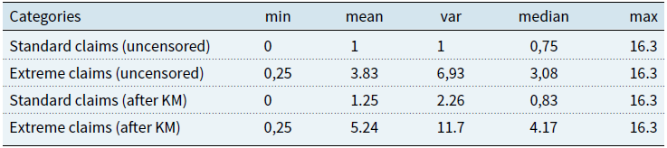
The database we consider gathers 113,072 claims from a French insurer, and corresponding expert reports describing the circumstances. These reports have been established at the opening of the claim, and do not take into account counter-expertises. Amongst these claims, 23% are still open (censored) at the date of extraction. Empirical statistics on the duration of a claim T are shown in Table 1.
Empirical statistics on the variable T, before and after correction by Kaplan–Meier weights (“after KM”). The category “Extreme claims” corresponds to the situation where  $I=1$ for
 $x=3\%$ of the claims, while “Standard claims” refers to the 97% lower part of the distribution of the final amount

For the claims that are closed, different severity indicators are known. These severity indicators have been previously computed from the final amount of the claim:  $I=1$ if the claim amount exceeds some quantile of the distribution of the amount, corresponding to the
 $x\%$ upper part of the distribution. In the situation we consider, this percentage x ranges from
 $1.5$ to 7, which means that we focus on relatively rare events, since
 $I=0$ for the vast majority of the claims.
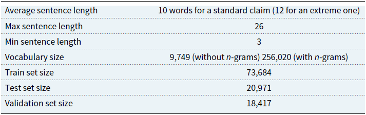
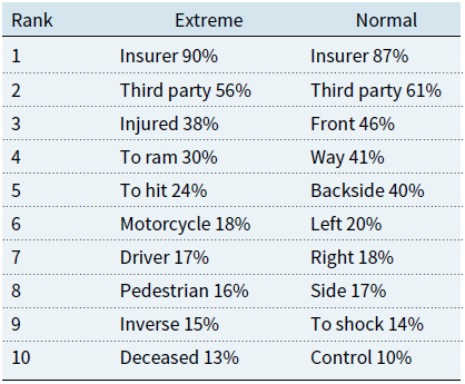
Some elements about the structure of the reports are summarised in Table 2 below. To get a first idea of which terms in the report could indicate severity, Table 3 shows which are the most represented words, distinguishing between claims with  $I=1$ and claims with
 $I=0.$
Summarised characteristics of the reports. The dataset is split into the train set (containing the observations used to fit the parameter of the network), the validation set (used to tune the hyperparameters), and the test set (used to measure the quality of the model). The vocabulary size “with n-grams” is the total of 1-grams, 2-grams and 3-grams

Ranking of the words (translated from French) used in the reports, depending on the category of claims (Extreme corresponds to  $I=1$ and Standard to
 $I=0.$)

In both cases, the two most frequent words are “insurer” and “third party”, which have to be linked with the guarantee involved. For extreme claims, we notice a frequent presence of a term related to a victim, for example, motorcycle or pedestrian. In addition there are also words related to the severity of the condition of a victim, such as injured or deceased. Moreover, two verbs are present in our top, “to ram” (we used this translation of the French verb “percuter”) and “to hit” (in French, “frapper”), which are related to some kind of violence of the event. On the other hand, for “standard” claims, the most frequent words are related to the car. Hence, reports on extreme claims use the lexical field of bodily damage, while the others use the terminology related to material damage.
Let us give two examples of phrases for each category (standard claim and severe claim):
standard claim:
1. pile-up on the road, 58 vehicles involved.
2. Insured gets hit at the rear, shock to the rear bumper.
Extreme claim:
3. insured hits the solid ground of a roundabout and dies during the transfer to emergency.
4. Third party does not stop at a stop sign and hits the insured in the front right, air bag triggered.
As one can see from these example, one of the specificities is that reports are often written in a short way, with a syntax which can sometimes be very brief. The vocabulary is also very specific to car insurance. On the other hand, in the third example, one can see that the conclusion that the claim is severe is obvious, since someone died. But example 4 is less obvious. A shock in the front is reported, but without explicit reference to the state of the victims, identification of such a claim as severe is expected to be much harder.
5.2 Hyperparameters of the networks and type of embedding
Let us recall that our procedure is decomposed into three steps:
A preliminary treatment to correct censoring (Kaplan–Meier weighting);
Embedding (determination of some appropriate metric between words);
Prediction, using the embedded words as inputs of a neural network. Depending on the embedding strategy, the prediction phase is either disconnected from the embedding (static method) or done at the same time (after a FastText initialisation, non-static method, or a random initialisation, random method).
For the last phase, we use LSTM and CNN described in section 4. For each of these architectures, we compare the different variations (static, non-static and random). The static and non-static classes of method are expected to behave better, taking advantage of a pre-training via FastText. For the LSTM networks, we consider two cases: when the words are decomposed into n-grams ( $n=1,2,3$) or without considering n-grams. In each case, the idea is to measure the influence of the different rebalancing strategies.
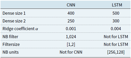
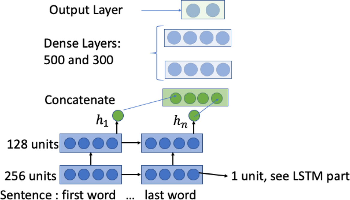
The weights in each of the networks we consider are optimised using the Adagrad optimiser, see Duchi et al. (Reference Duchi, Hazan and Singer2011). Training is done through stochastic gradient descent over shuffled mini batches with the Adagrad update rule. The architecture and hyperparameters of the LSTM and CNN are shown in Table 4 and Figures 7 and 8 below. A ridge regularisation is applied to the layer kernel of the output layer, that is introducing a  $L^2$-penalty multiplied by a penalisation coefficient
 $\alpha$. These parameters are used in every CNN/LSTM model that is considered. The codes are available on https://github.com/isaaccs/Insurance-reports-through-deep-neural-networks.
Hyperparameters of the RNN used in the real data analysis

Representation of the CNN network used in the real data analysis.

Representation of the LSTM network used in the real data analysis. The output of the network is followed by a multilayer perceptron.

Our model is implemented using Tensorflow, see Abadi et al. (Reference Abadi, Agarwal, Barham, Brevdo, Chen, Citro, Corrado, Davis, Dean, Devin, Ghemawat, Goodfellow, Harp, Irving, Isard, Jia, Jozefowicz, Kaiser, Kudlur, Levenberg, Mané, Monga, Moore, Murray, Olah, Schuster, Shlens, Steiner, Sutskever, Talwar, Tucker, Vanhoucke, Vasudevan, Viégas, Vinyals, Warden, Wattenberg, Wicke, Yu and Zheng2015), on Python for deep learning models, and we use sk-learn, see Pedregosa et al. (Reference Pedregosa, Varoquaux, Gramfort, Michel, Thirion, Grisel, Blondel, Prettenhofer, Weiss, Dubourg, Vanderplas, Passos, Cournapeau, Brucher, Perrot and Duchesnay2011), for the Machine Learning models.
5.3 Performance indicators
In this section, we describe the criteria that are used to compare the final results of our models. Due to the small proportion of observations such that  $I=1,$ measuring the performance only by the well-predicted responses would not be adequate, since a model which would systematically predict 0 would be ensured to obtain an almost perfect score according to this criterion. Let us introduce some notations:
TN is the number of negative examples (
$I=0$) correctly classified, that is “True Negatives”.FP is the number of negative examples incorrectly classified as positive (
$I=1$), that is “False Positives”.FN is the number of positive examples incorrectly classified as negative (“False Negatives”).
TP is the number of positive examples correctly classified (“True Positives”).


We then define Recall and Precision as
 \begin{eqnarray}\textrm{Recall} & = & \frac{TP}{TP+FN}, \nonumber \\[5pt]\textrm{Precision} & = & \frac{TP}{TP+FP} \nonumber\end{eqnarray}
So, Recall is the proportion of 1 that have been correctly predicted with respect to the total number of 1. For Precision, the number of correct predictions of 1 is compared to the total of 1-predicted observations.  $F_1$-score (see, for example, Akosa, Reference Akosa2017) is a way to combine these two measures, introducing
 \begin{equation*}F_1=\frac{2\times Recall\times Precision}{Recall+Precision}\end{equation*}
The  $F_1$-score conveys the balance between the precision and recall.
Remark:  $F_1$-score is a particular case of a more general family of measures defined as
 \begin{equation*}F_\beta=\frac{(1+\beta^2)\times Recall\times Precision}{Recall+\beta^2\times Precision}\end{equation*}
where  $\beta$ is a coefficient to adjust the relative importance of precision versus recall, decreasing
 $\beta$ leads a reduction of precision importance. In order to adapt the measure to cost-sensitive learning methods, Chawla et al. (Reference Chawla, Bowyer, Hall and Kegelmeyer2002) proposed to rely on
 \begin{equation} \beta=\frac{c(1,0)}{c(0,1)}\end{equation}
where c(1,0) (resp. c(0,1)) is the cost associated to the prediction of a False Negative (resp. of a False Positive). The rationale behind the introduction of such  $F_{\beta}$ measure is that misclassifying within the minority class is typically more expansive than within the majority class. Hence, considering the definition (6) of
 $\beta,$ improving Recall will more affect
 $F_{\beta}$ than improving Precision. In our practical situation, it was difficult to define a legitimate cost for such bad predictions, which explains why we only considered
 $F_1$-score amongst the family of
 $F_{\beta}$-measures.
5.4 Results
As we have already mentioned,  $I=1$ corresponds to a severe event, that is the loss associated with the claim corresponds to the
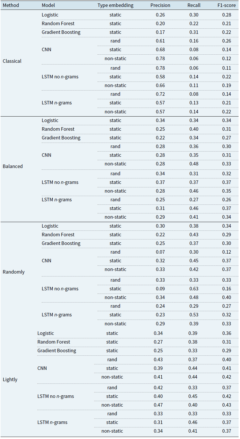
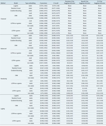
 $x\%$ upper part of the loss distribution. We made this proportion vary from 1.5% to 7% to see the sensitivity to this parameter. Table 5 shows the benefits of using the different resampling algorithms of section 2.3 in the case where the proportion of 1 in the sample is 3% (which is an intermediate scenario considering the range of values for x that we consider). The neural networks methods are benchmarked with a classical logistic predictor, and two other competing machine learning methodology (Gradient Boosting and Random Forests, see Friedman et al., Reference Friedman, Hastie and Tibshirani2001). To make think comparable, all these alternatives methodologies are combined with the FastText embedding (as in the static methods). Moreover, we apply the same resampling algorithms of section 2.3 to these methods. For Algorithm 4, we considered a balanced case, where the proportion of 1 in the bootstrap samples is 50%, and a “lightly” rebalanced case where these proportion is only 10%. This choice of 10% was motivated by Table 1 in Verdikha et al. (Reference Verdikha, Adji and Permanasari2018): it corresponds to a situation that the authors qualify as “moderately imbalanced”, instead of “extremely imbalanced”. In Table 6, confidence intervals (CI) are provided for the performance indicators.
Influence of the constrained bagging algorithms of section 2.3. For “Classical,” no rebalancing algorithm has been used. “Balanced” corresponds to algorithm 2.3 with an equal proportion of 1 and 0 in each sample. “Randomly” corresponds to algorithm 3 with an equal proportion (in average) of 1 and 0 in each sample. “Lightly” corresponds to Algorithm 4 with 10% of 1 (in average) in each sample. In the Random Forest algorithm, we used 200 trees, with a Gini criterion and a maximal depth of 3. In the Gradient Boosting algorithm, 200 trees were used, and a deviance loss with a learning rate of 0.1

CI of the scoring. The CI for Precision and Recall (columns 4 and 5) are computed using a beta distribution following the methodology of Goutte & Gaussier (Reference Goutte and Gaussier2005). For bagging (columns 6–8), the CI is based on percentile bootstrap following Hesterberg (Reference Hesterberg2014)

Let us first observe that the network methodologies lead to a relatively good precision if one does not use rebalancing strategies. This is due to the fact that precision only measures the proportion of true positive amongst all the claims that have been predicted to be 1. Typically, the networks methodologies, in this case, predict correctly the “obviously” severe claims, but miss lots of these severe claims. This explains why recall and  $F_1$-score are much lower.
The rebalancing algorithm mostly benefit the machine learning methodologies. One also observes that the embedding methodologies based on FastText (static and non-static methods) leads to better performances. The performance of all techniques in terms of  $F_1$-score is not spectacular (in the sense that it is not close to 1), but this has to be related with the complexity of the problem (predicting a relatively rare class of events). Compared to the basic logistic method (after embedding), the best network (LSTM without considering n-grams, with the lightly balanced bagging algorithm) leads to an improvement of 20% in terms of
 $F_1$-score.
Let us also observe that the LSTM network architecture, which does not rely on n-grams behaves better than the LSTM which actually uses these n-grams. This may be counterintuitive, since the use of n-grams is motivated by the idea that one could use them to take the context of the use of a word into account. Nevertheless, considering n-grams increases the number of parameters of the network, while context information is already present in the embedding methodologies. On the other hand, CNN methods have lower performance than LSTM ones, but the performances stay in the same range (with a computation time approximatively four times smaller to fit the parameters of the network).
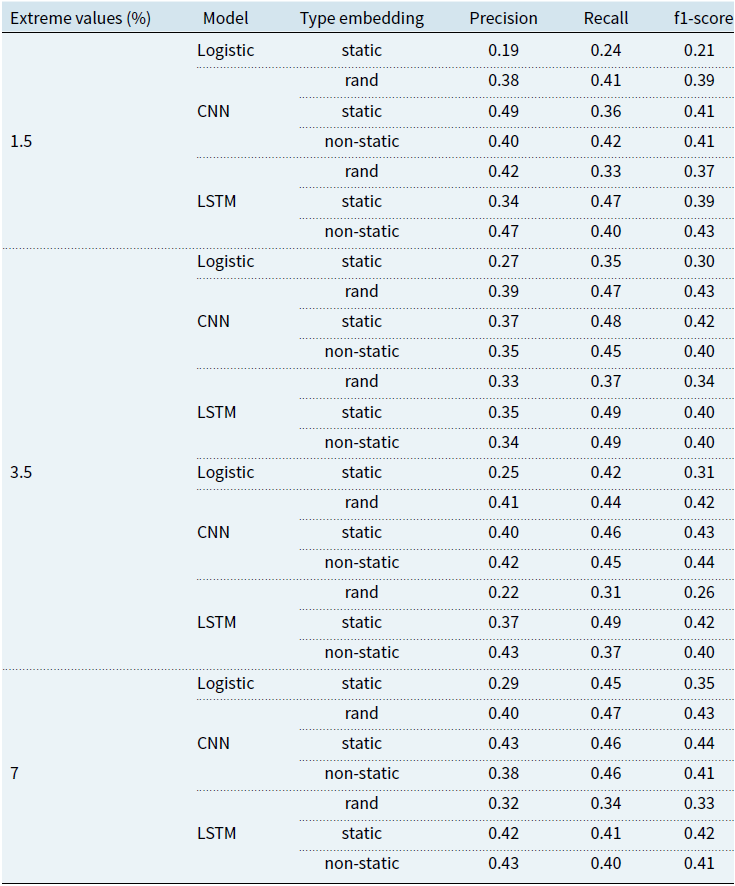
Table 7 shows the influence of the proportion x on the performance (we only report a selected number of methods for the sake of brevity. We observe that the performance of the logistic method decreases with the proportion of 1 contained in the sample. On the other hand, the network-based methods’ performance stay relatively stable.
Performance of the different methodologies (combined with the different embedding technics). The first column indicates the percentage of 1 in the sample

5.5 Alternative methods for text analysis of imbalanced data
Amongst the techniques that are frequently used when it comes to dealing with imbalanced data, SMOTE, see Chawla et al. (Reference Chawla, Bowyer, Hall and Kegelmeyer2002), has not been used in our context, because this approach is designed for image and not adapted to text analysis. ForesTexter, see Wu et al. (Reference Wu, Ye, Zhang, Ng and Ho2014), is an algorithm based on random forests which can be used for text categorisation, with promising results. Therefore, we compared the results of our approach with ForesTexter. Through this method, we obtained a Precision of 0.58, a Recall of 0.07 and a F1-Score of 0.12 (when the percentage of 1 is 3%).
Hence, the Precision is much better for ForesTexter. This means that, when ForesTexter predicts an extreme claims, it tends to be right (at least, more than with our procedure). On the other hand, it has a poor performance in terms of Recall, which means it tends to “under-detect” these extreme claims. In other words, this approach tends to only detect obvious extreme claims. For insurance applications, the F1-Score seems a much adapted metric.
6 Conclusion
In this paper, we proposed a detailed methodology to perform automatic analysis of text reports in insurance, in view of predicting a rare event. In our case, the rare event is a particularly severe claim. This question of clustering such claim is of strategic importance, since it allows to operate a particular treatment of the claims that are identified as “extreme”. Four steps of our method are essential:
correction of censoring via survival analysis techniques;
compensation of the rarity of the severe events via rebalancing bagging techniques;
a proper representation of the words contained in the reports via an appropriate embedding technique;
the choice of a proper neural network architecture.
LSTM networks, associated with a performant embedding method, appear to be promising tools to perform this task. Nevertheless, learning rare events is still a hard task, especially in such insurance problem where the volume of data is limited, especially when dealing with such a specific vocabulary. Insurance is, of course, not the only sector where specific terminologies can influence the behaviour of such techniques, see, for example, Lee et al. (Reference Lee, Yoon, Kim, Kim, Kim, So and Kang2020) for similar biomedical problematics. The integration of additional variables to increase the information on the claims should be essential to improve the prediction. Moreover, let us mention that, in this work, we only considered information available at the opening of the claim to predict its outcome. For long development branches, the incorporation of updated information on the evolution of the claims could be determinant and should be incorporated in the methodology.
Acknowledgements
The author acknowledge the support of Crédit Agricole Assurances and of Agence Nationale de la Recherche et de la Technologie (ANRT).
A Appendix
A.1 Typical choices of activation functions for neural networks
A list of typical activation functions is provided in Table A.1.
Typical choices of activation functions

A.2 Additional type of layers in a CNN
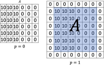
Zero padding. Zero padding is the simplest way to avoid diminishing too much the dimension of the input when going deeper into the network. As we can see above in Figure 3, a convolution step will produce an output C of smaller dimension than A. Moreover, when dealing with our text data, it is useful to control the size of our inputs. Let us recall that we want to automatically analyse reports to predict the severity of a claim. These reports do not all have the same size in terms of words. Zero padding creates a larger matrix by adding zeros on the boundaries, as shown in the example of Figure A.1. Similar issues are present when dealing with images that may not all have the same number of pixels.
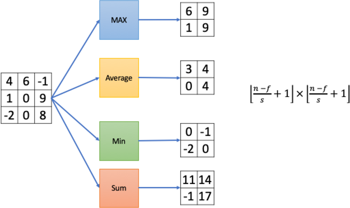
Pooling Step. Pooling steps work similarly as convolution layers, but applying locally a function that may not be linear. An example is shown in Figure A.2.
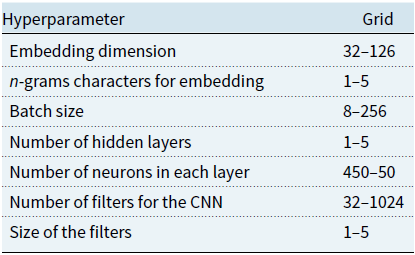
Range of values on which the hyperparameters have been optimised

Let us note that, in the example of Figure A.2, the functions “Average” and “Sum” may be seen as linear filters, as shown in Figure 3 (for example, function “Sum” is related to a filter B whose coefficients are all 1). The only difference is that the parameters of a convolution layer evolves through the calibration process of the network, while the coefficients of a pooling layer are fixed.
A.3 Hyperparameters
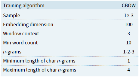
We list below the hyperparameters used in the different networks. A grid search has been used to determine which set of hyperparameters lead to the best performance. Table A.2 lists the range of values on which the optimisation has been done. The embedding dimension denotes the dimension N after reduction of the vocabulary V. Batch size is a parameter used in the Batch Gradient Descent (used in the algorithm of optimisation of the weights of the networks), see Bengio (Reference Bengio2012). The number of hidden layers refer to the final multilayer perceptron block used at the output of LSTM and CNN networks. A separate Table (see Table A.3 is devoted to the parameters involved in the embedding part of the procedure.
Hyperparameters of the embedding matrix used in the real data analysis

Zero padding.

Example of a pooling layer: each function is applied to a moving square of input coefficients of size  $2\times 2$.

All the codes are available at the following url:
https://github.com/isaaccs/Insurance-reports-through-deep-neural-networks.