1. Introduction
Liquid foams are dense dispersions of gas bubbles in a continuous liquid phase containing surfactants to ensure their stability. The bubbles are in contact through thin soap films, supported by an interconnected network of liquid channels (also called Plateau borders). Foams exhibit a peculiar rheology, with finite yield stress and shear modulus, a high effective viscosity and non-Newtonian behaviour. The link between these characteristics of liquid foams, which make them useful in a variety of industrial applications (Stevenson Reference Stevenson2012), and their structure has been thoroughly investigated, both experimentally and theoretically, in the regime of small to intermediate strain rates and frequencies (up to a few tens of Hz) (see Cohen-Addad, Höhler & Pitois Reference Cohen-Addad, Höhler and Pitois2013 and Dollet & Raufaste Reference Dollet and Raufaste2014 for recent reviews).
These shear rates and frequencies remain lower, however, than those achieved in many industrial applications, such as the mitigation of shock and blast waves by aqueous foams (Goldfarb et al.
Reference Goldfarb, Orenbakh, Shreiber and Vafina1997; Britan, Liverts & Ben-Dor Reference Britan, Liverts and Ben-Dor2009; Del Prete et al.
Reference Del Prete, Chinnayya, Domergue, Hadjadj and Haas2013) and the design of new probes of liquid foams based on their acoustic response. A related subject is the propagation of acoustic waves through foams, which surprisingly has been considered only rather recently (Moxon, Torrance & Richardson Reference Moxon, Torrance and Richardson1988; Mujica & Fauve Reference Mujica and Fauve2002; Kann Reference Kann2005; Pierre et al.
Reference Pierre, Guillermic, Elias, Drenckhan and Leroy2013; Pierre, Dollet & Leroy Reference Pierre, Dollet and Leroy2014). Most experimental studies (Mujica & Fauve Reference Mujica and Fauve2002; Pierre et al.
Reference Pierre, Guillermic, Elias, Drenckhan and Leroy2013) report low values for the speed of sound (of the order of 50 m s
 $^{-1}$
), in agreement with mean field models that predict the speed of sound from the average density and compressibility of the foam (Wood Reference Wood1944). However, much higher sound velocities (of the order of 200 m s
 $^{-1}$
) have also been measured (Moxon et al.
Reference Moxon, Torrance and Richardson1988), and dedicated models (Kann Reference Kann2005) have been proposed, describing the sound propagation as occurring in the gas phase only, except for the additional inertia provided by the soap films. These different viewpoints have been unified in a recent study (Pierre et al.
Reference Pierre, Dollet and Leroy2014), which proposed a model based on a description of the vibration of the foam structure in response to the propagation of a pressure wave. It showed that at low frequency and/or small bubble size, the films and Plateau borders vibrate in phase and with the same amplitude, justifying the mean field approach. At high frequency and/or large bubble size, the vibration amplitude of the Plateau borders is negligible compared to that of the soap films, because of the huge difference in their inertias, thereby justifying the model of Kann (Reference Kann2005).
However, although the model of Pierre et al. (Reference Pierre, Dollet and Leroy2014) gives satisfactory agreement with experimental measurements, it is not possible to check in situ whether the vibrational response of the films and Plateau borders agrees with the model, because of the opacity of the foams and the high frequencies involved. To do so requires an experiment where the coupled vibrations of films and Plateau borders in response to an acoustic forcing can be directly visualised and measured.
Film vibration has been investigated by several groups: see, for example, Taylor (Reference Taylor1959), Couder, Chomaz & Rabaud (Reference Couder, Chomaz and Rabaud1989), Afenchenko et al. (Reference Afenchenko, Ezersky, Kiyashko, Rabinovich and Weidman1998), Vega, Higuera & Weidman (Reference Vega, Higuera and Weidman1998), Boudaoud, Couder & Ben Amar (Reference Boudaoud, Couder and Ben Amar1999), Elias, Hutzler & Ferreira (Reference Elias, Hutzler and Ferreira2007) and Kosgodagan Acharige, Elias & Derec (Reference Kosgodagan Acharige, Elias and Derec2014). Taylor (Reference Taylor1959) introduced the possible modes of vibration for a film: a symmetric mode, with thickness modulations, and an asymmetric bending mode, where the film retains a constant thickness. Films usually vibrate in a bending mode that is less dissipative than the symmetric mode. At low frequencies, simple flexural waves are observed; for a circular film, they take the form of circular rings. At higher frequencies, vortical structures develop inside the vibrating films (Couder et al. Reference Couder, Chomaz and Rabaud1989; Afenchenko et al. Reference Afenchenko, Ezersky, Kiyashko, Rabinovich and Weidman1998; Vega et al. Reference Vega, Higuera and Weidman1998; Elias et al. Reference Elias, Hutzler and Ferreira2007). At high amplitudes, nonlinear effects arise, such as self-adaptation of the film thickness to adopt a resonant configuration whatever the frequency (Boudaoud et al. Reference Boudaoud, Couder and Ben Amar1999), which eventually leads to film rupture (Drenckhan et al. Reference Drenckhan, Dollet, Hutzler and Elias2008).
All the aforementioned experiments were done with films tethered to a rigid frame. There are also some scattered observations of the coupled vibrations of films and Plateau borders. As a model system for foam rheology, Besson & Debrégeas (Reference Besson and Debrégeas2007) studied the oscillations of two soap bubbles in contact, forced by a sinusoidal modulation of the distance between their two centres, and quantified the modulation of the contact angle between the two bubbles. However, they did not study the vibration of the film separating the two bubbles. Hutzler et al. (Reference Hutzler, Saadatfar, van der Net, Weaire and Cox2008) studied a Plateau border created following a topological rearrangement between adjacent films. They showed that the new Plateau border grows and displays free oscillations with a characteristic frequency and damping, and suggested that air inertia is crucial to understanding this dynamics; however, no systematic study of the coupled vibration of a free film connected to a Plateau border has been undertaken.
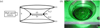
Several recent works have attempted to rationalise the coupled dynamics of the air, the soap films and the Plateau border. These studies differ by the geometry investigated and by the amplitude of the forcing. Elias et al. (Reference Elias, Kaurin, Arbogast, Leroy, Gay and Derec2015) investigated the case of a linear Plateau border that is transversally vibrated, and they measured and modelled the dispersion relation of the transverse waves for a low amplitude of forcing. For a higher forcing amplitude, Cohen, Fraysse & Raufaste (Reference Cohen, Fraysse and Raufaste2015) observed the modulation of the cross-sectional area of the Plateau border in response to the vibration. In both studies, the Plateau border is long enough that several wavelengths exist along it. In the present paper, we address this issue by considering a model minimal configuration, the diaboloid (Salkin et al. Reference Salkin, Schmit, Panizza and Courbin2014), consisting of two films (henceforth called the suspending films) each connected to a circular ring and taking the shape of a catenoid, connected to each other by a planar soap film, henceforth called the suspended film (see figures 1 a and 2 a). This is a model system for our purposes, since the liquid meniscus at the intersection of three films mimics the Plateau border in foams, and the suspended film is freely suspended between this meniscus (as opposed to being rigidly tethered to a solid ring). This configuration has been used by Seiwert et al. (Reference Seiwert, Monloubou, Dollet and Cantat2013) to study the behaviour of such a suspended film under extension.
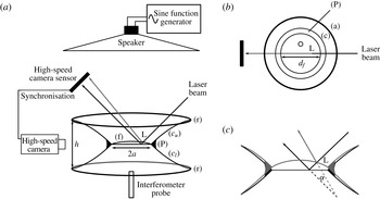
(a) Experimental set-up for free oscillations (not to scale): the suspended film (f), of thickness
 $e\approx 0.5{-}1.5~{\rm\mu}\text{m}$
and diameter
 $2a\approx 14{-}20~\text{mm}$
, is suspended between two aluminium rings (r) (22 mm in diameter) placed a distance
 $h$
apart via an upper suspending film (
 $c_{u}$
) and a lower suspending film (
 $c_{l}$
); the three films meet at the Plateau border (P), at an angle of approximately 120°; (P) is backlit and its profile is monitored by a high-speed camera. (b) Close-up of the rings: the suspended film (f) is lit with a monochromatic lamp, which produces the interference pattern seen in the picture.

The paper is organised as follows. In § 2, we describe our set-up and quantify the eigenfrequency and damping of the free oscillations of the Plateau border. In § 3, we introduce a model of coupled oscillations of the suspended film and the Plateau border, which predicts the experimental eigenfrequencies with no fitting parameter. In § 4, we extend our set-up to study the forced response of the suspended film and of the Plateau border to a sound field, and we measure resonance curves of the suspended film. We discuss this resonance in § 5 through a simple extension of the previous model. In particular, we show the importance of the coupling between the film and the Plateau border.
2. Free oscillations: experiments
2.1. Set-up
The axisymmetric system we study (sketched in figure 1) is a diaboloid, composed of three films: a horizontal circular film, denoted by (f), connected via two catenary films, denoted by (
 $c_{u}$
) and (
 $c_{l}$
), to two aluminium rings (21 mm in diameter, one above and one below) separated by a distance
 $h$
; the three films meet at a circular meniscus, called the Plateau border. This set-up is adapted from our recent study of soap film extension (Seiwert et al.
Reference Seiwert, Monloubou, Dollet and Cantat2013). To create the diaboloid, the solid rings are first placed in close proximity to each other (
 $h\approx 0.5$
mm) and then dipped into a foaming solution of 10 g l
 $^{-1}$
sodium dodecyl sulfate (SDS) in water or a water/glycerol mixture. This creates a single (horizontal) film attached to both of the rings. The upper and lower suspending films appear naturally when the rings are separated to reach their final position (
 $h$
varies between 2.8 and 6.3 mm depending on the experiment).
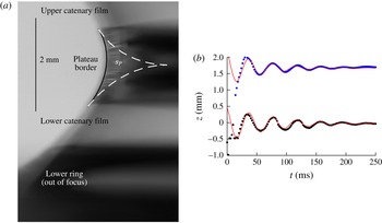
(a) Typical profile image of the Plateau border, from which we extract its radius (by fitting) and the position of its upper and lower boundaries. (b) Positions of the upper and lower boundaries of the Plateau border, plotted as functions of time, during a free oscillation experiment (with
 $h=4.8$
mm and
 $s_{P}=0.4~\text{mm}^{2}$
). Solid lines represent best fits of the form (2.1):
 $z(t)=z_{0}+A_{0}\,\text{e}^{-2{\rm\pi}lf_{0}t}\,\sin (2{\rm\pi}f_{0}\sqrt{1-l^{2}}\,t)$
with best-fit parameters
 $f_{0}=25$
Hz and
 $l=0.12$
(upper) or
 $l=0.087$
(lower).

A key parameter of our system is the cross-sectional area of the Plateau border. We measure it by imaging the system from the side (figure 2
a) and fitting the external profile (the rim) of the Plateau border. The fit takes into account axisymmetry, surface tension and gravity, and allows us to determine the cross-sectional area of the Plateau border
 $s_{P}$
, which measures the Plateau border size. The fitting procedure leads to a relative uncertainty in
 $s_{P}$
of at most 6 %. This relative uncertainty is obtained by comparing the fitted cross-section to the following cruder estimation. The rim of the Plateau border is fitted by a circular arc of radius
 $R_{P}$
, which would be its shape in the absence of gravity; the cross-section of the Plateau border would then equal
 $(\sqrt{3}-{\rm\pi}/2)R_{P}^{2}$
(Dollet & Raufaste Reference Dollet and Raufaste2014). We have checked that the relative difference between this crude estimate and the more complete fit does not exceed 6 %. The method used to prepare the system creates a ‘thick’ Plateau border of cross-sectional area
 $s_{P}\simeq 0.6$
mm
 $^{2}$
. This can be adjusted down to a minimal cross-sectional area of
 $s_{P}\simeq 0.05$
mm
 $^{2}$
, although not in a finely controllable way, by sucking out some of the liquid with a paper tissue.
Under the action of the capillary suction at the Plateau border, the central film is constantly draining throughout the experiment. By waiting at least one minute between film formation and the experiment itself, we ensure that the thinning of the film has slowed down enough to be negligible (i.e. less than 5 % variation in thickness over the time needed to perform the measurements, typically 10 s). We also systematically measure the film thickness with a reflectometer just prior to starting the experiment.
We performed two different types of experiment. First, in free oscillations experiments, we perturb the position of the Plateau border and observe it as it returns towards equilibrium, gathering data on the fundamental eigenfrequency and the damping of the system. Second, in forced oscillations experiments, a sinusoidal sound wave is used to excite the system at a given frequency. We will return to forced oscillations from § 4 onwards; let us first focus on free oscillations.
To generate the perturbation, we first create the three films with a distance
 $h=6.3$
mm between the rings, and then suddenly raise the lower ring with a motorised stage (in approximately 25 ms) until
 $h=2.8$
or 4.8 mm. The inertia of the Plateau border ensures that it does not move significantly over this short period of time, so just after ring displacement it rests with negligible velocity approximately 1.75 mm away from its new equilibrium position. We image the system from the side with a high-speed camera (at 100–500 f.p.s., with a typical image shown in figure 2
a), and track the position of the upper and lower boundaries of the Plateau border as a function of time.
As shown in the example of figure 2(b), the two boundaries move in phase with the same amplitude. They oscillate around their new equilibrium positions, and come to rest after a few oscillations. Except at short times, the movement is well fitted by an exponentially decaying sinusoid of the form
 $$\begin{eqnarray}z=z_{0}+A_{0}\,\text{e}^{-2{\rm\pi}lf_{0}t}\,\sin (2{\rm\pi}f_{0}\sqrt{1-l^{2}}\,t),\end{eqnarray}$$
which is the expression for the unforced damped oscillations of an underdamped harmonic oscillator of eigenfrequency
 $f_{0}$
and damping coefficient
 $l$
. In particular, the period remains constant to within 10 %. The damping coefficient and the eigenfrequency of these free oscillations are found by fitting the data, and they characterise each experiment. When analysing the data, we fit independently the upper and lower boundaries and plot their mean value (with error bars spanning the entire range).
To validate the set-up, we first performed a series of test experiments to check that
 $f_{0}$
and
 $l$
do not depend on the method used to drive the Plateau border out of equilibrium. In particular, we tested two different displacement speeds for the ring, and found no difference except for a short transient. We also checked that the film remains flat in these experiments and follows the Plateau border.
2.2. Results
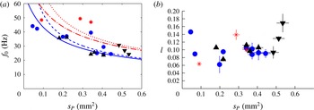
We plot in figure 3(a) the eigenfrequency
 $f_{0}$
as a function of the Plateau border cross-sectional area
 $s_{P}$
. The eigenfrequency varies between 10 and 50 Hz, and decreases with
 $s_{P}$
. Additionally,
 $f_{0}$
increases when the gap between the rings goes from
 $h=4.8$
mm (solid symbols) to
 $h=2.8$
mm (asterisks). The damping coefficient
 $l$
is shown in figure 3(b). The data are more scattered, because the fit for
 $l$
is more sensitive to experimental errors (especially in the tracking of the Plateau border). However, there is no systematic variation of
 $l$
with
 $s_{P}$
.
(a) Eigenfrequency
 $f_{0}$
and (b) damping coefficient
 $l$
measured by fitting free oscillations of the Plateau border as a function of its cross-sectional area
 $s_{P}$
. Asterisks are for
 $h=2.8~\text{mm}$
, while all other symbols are for
 $h=4.8~\text{mm}$
. Asterisks and circles are for solution S (10 g l
 $^{-1}$
SDS in water); upward and downward triangles are for solutions S50 and S80, containing 50 % and 80 % of glycerol, respectively. For each experiment, the upper and lower boundaries are fitted independently, as illustrated in figure 2(b), and error bars span the two extracted values. The solid and dashed lines are, respectively, the predictions (with no fitting parameter) for the eigenfrequency
 ${\it\Omega}_{P}/(2{\rm\pi})$
, with
 ${\it\Omega}_{P}$
given by (3.6) of the Plateau border, and the fundamental frequency of the coupled system (see § 3.4), for
 $h=4.8$
mm. Similarly, the dash-dotted and dotted lines are, respectively, the predictions for the eigenfrequency
 ${\it\Omega}_{P}/(2{\rm\pi})$
, with
 ${\it\Omega}_{P}$
given by (3.6) of the Plateau border, and the fundamental frequency of the coupled system, for
 $h=2.8$
mm.

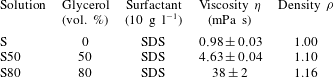
We also tested different foaming solutions, all containing 10 g l
 $^{-1}$
of SDS dissolved in a 0 %, 50 % or 80 % glycerol/water mixture. The main difference between these three solutions is their shear viscosity
 ${\it\eta}$
, which goes roughly from 1 to 40 mPa s (see table 1). They also show a small difference in their density
 ${\it\rho}$
. This large increase in shear viscosity, however, does not translate into an increase in the damping coefficient (figure 3
b).
Foaming solutions used in the experiments, together with their measured physical properties. The surface tension
 ${\it\gamma}=32~\text{mN}~\text{m}^{-1}$
is the same for all solutions.

3. Free oscillations: interpretation
3.1. Simplifying assumptions
The upper and lower suspending films determine the equilibrium position of the Plateau border, and for small displacements around the equilibrium position, we expect that the suspending films will act as a capillary spring. Together with the mass of the Plateau border and the film, this sets an eigenfrequency.
To further develop and evaluate this idea, let us write explicitly the balance between inertia and capillarity, which allows us to predict, with no fitting parameter, the observed eigenfrequency (as seen in figure 3 a). In particular, we show in the next subsection that the dynamics of the film has to be taken into account. Our model is based on several approximations.
-
(1) The problem is purely axisymmetric.
-
(2) The thickness
 $e$
of the suspended film remains uniform at all times.
-
(3) The Plateau border is a rigid ring of radius
$a$
and cross-sectional area
$s_{P}$
much smaller than
$a^{2}$
. The mass per unit length of this ring is
${\it\mu}={\it\rho}s_{P}$
. Moreover, its weight is neglected, so that the only forces acting on it are the capillary tractions of the three films. -
(4) The oscillations of the Plateau border and the film are much smaller than the separation between the rings (and are treated at first order).
-
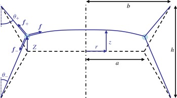
(5) The curvature of the suspending films in the diametral plane is negligible (figure 4). Hence, the capillary equilibrium imposes a 120° angle between the suspending films, yielding the following geometrical relation between the film radius
$b$
of the supporting rings, the radius
$a$
of the Plateau border and the gap
$h$
between the two supporting rings:
$b=a+h/2\sqrt{3}$
. -
(6) All forms of dissipation (viscous dissipation in the liquid and in the air, thermal dissipation in the air, radiation damping) are neglected.


We now discuss the validity of these approximations. Approximation (1) is validated by analysing experimental movies, and indeed no deviation from axisymmetry, in either the film or the Plateau border, is observed during free oscillations.
Sketch of the films in a diametral plane (not to scale). The dash-dotted line is the axis of revolution of the system. The dashed lines represent the assumed equilibrium configuration; see § 3.1. The Plateau border is sketched as the light blue circle at the junction of the films. Its motion is forced by the tractions
 $\boldsymbol{f}_{+}$
,
 $\boldsymbol{f}_{-}$
and
 $\boldsymbol{f}$
of the three films to which it is connected, respectively the upper suspending film, the lower suspending film and the suspended film.

Assumption (2) is also validated by direct visualisation of the system during a specific set of validating experiments, with a slightly different imaging set-up than what is shown here. In order to observe the evolution of the thickness of the suspended film, the film is illuminated by a monochromatic light, which reflects off both interfaces of the film and produces an interference pattern, as seen in figure 1(b). Imaging the film from above thus gives us a time-resolved map of the relative thickness of the film. There are some local heterogeneities in thickness, but we have checked that there are no large-scale thickness gradients.
For the Plateau border to be represented by a ring of negligible cross-sectional area, as in assumption (3), its characteristic length scale
 $\sqrt{s_{P}}$
must remain negligible compared to both the radius
 $a$
of the film and the distance
 $h$
between the rings. In our experiments,
 $\sqrt{s_{P}}$
reaches at most 1 mm, while
 $a\approx 8$
mm and
 $h\approx 5$
or 3 mm. The condition
 $\sqrt{s_{P}}\ll a$
is thus satisfied to within 12 %. The condition
 $\sqrt{s_{P}}\ll h$
is more questionable, particularly for the smallest distance between rings. However, the finite extent of the Plateau border is known not to modify the orientation of the films (apart from its weight, which we discuss next), a result known as the decoration theorem (Weaire & Hutzler Reference Weaire and Hutzler1999). Therefore, the forces exerted by the films should remain independent of the cross-sectional area of the Plateau border, even if
 $\sqrt{s_{P}}/h$
is not particularly small.
Neglecting the weight of the Plateau border may seem questionable, as seen in figure 2(a): the main effect of gravity is to desymmetrise the equilibrium position of the system, and the upper film is slightly more vertical than the lower one. To assess this approximation in terms of force balance, we must compare the weight per unit length,
 ${\it\mu}g$
, to the tractions per unit length,
 $2{\it\sigma}$
, exerted by each of the films. In our experiments,
 $s_{P}$
is below 0.6 mm
 $^{2}$
, so
 ${\it\mu}g/2{\it\sigma}$
remains below 0.1. Taking into account the finite weight of the Plateau border is in fact straightforward. We have checked that including it in the force balance presented in § 3.2 modifies the eigenfrequency by less than 6 %, which is comparable to the experimental uncertainties. Hence, we neglect weight for simplicity.
Approximation (4) is easily justified: the amplitudes of the oscillations of the Plateau border (typically 0.5 mm) and the film (at most 0.1 mm) are ten times smaller than the distance between the rings (
 $h\approx 5$
mm).
Approximation (5) is mainly imposed for convenience; taking into account the curvature of the suspending films (whose shape is a catenary, since their total curvature must be nil) is tedious but straightforward on a static diaboloid (Salkin et al. Reference Salkin, Schmit, Panizza and Courbin2014). By comparing the exact (curved) shape of a static diaboloid and the shape without curvature (dashed line in figure 4), we have calculated that our approximation leads to a slight overestimation of the film radius, by at most 5 %.
Lastly, assumption (6) follows directly from the small damping ratio (
 $l\approx 0.1$
) of the system. For small
 $l$
, the damping affects the eigenfrequency by a factor of order
 $l^{2}$
(Landau & Lifchitz Reference Landau and Lifchitz1969). Hence, we may safely assume the eigenfrequency to be almost independent of the exact value of the dissipation. Of course, this completely overlooks the microscopic mechanisms at the origin of the observed damping, which are discussed in appendix A.
3.2. Dynamics of the Plateau border
Let
 $z(r,t)$
be the vertical position of the films, and let
 $Z(t)\equiv z(a,t)$
be the vertical position of the Plateau border with respect to the equilibrium position
 $z=0$
(figure 4).
The motion of the Plateau border is driven by the capillary traction of the three films to which it is connected; each of these films exerts a force directed tangentially to the films (figure 4) and of magnitude
 $2{\it\sigma}$
. This comes from the fact that a given film is bounded by two air/liquid interfaces, with a surface tension
 ${\it\sigma}$
on each interface. Hence, the projections along the upward vertical direction (henceforth referred to as the vertical projections) of the force per unit length exerted by the upper and lower suspending films are, respectively,
 $f_{+z}=2{\it\sigma}\cos {\it\theta}_{+}$
and
 $f_{-z}=-2{\it\sigma}\cos {\it\theta}_{-}$
, where the projection angles
 ${\it\theta}_{\pm }$
are drawn in figure 4. Moreover, consistent with the assumption (4) of small oscillations, the vertical slope of the suspended film is such that
 $|\partial _{r}z|\ll 1$
. Hence, the vertical projection of the force per unit length exerted by the suspended film on the Plateau border is
 $f_{z}=-2{\it\sigma}\partial _{r}z(a,t)$
. Upon summing these three forces and vertically projecting Newton’s law, for a unit length of Plateau border of mass
 ${\it\mu}$
, we get
 $$\begin{eqnarray}{\it\mu}\ddot{Z}=f_{z}+f_{+z}+f_{-z}=-2{\it\sigma}\partial _{r}z(a,t)+2{\it\sigma}(\cos {\it\theta}_{+}-\cos {\it\theta}_{-}).\end{eqnarray}$$
Assumption (5) requires that the suspending films projected in a diametral plane be straight lines (figure 4). Hence, from simple geometry, we get
 $$\begin{eqnarray}\cos {\it\theta}_{\pm }=\frac{h/2\mp Z}{[(h/2\sqrt{3})^{2}+(h/2\mp Z)^{2}]^{1/2}}.\end{eqnarray}$$
Moreover, from assumption (4),
 $|Z|\ll h$
; hence, to first order in
 $|Z|/h$
,
 $$\begin{eqnarray}\cos {\it\theta}_{\pm }\simeq \frac{\sqrt{3}}{2}\left(1\mp \frac{Z}{2h}\right).\end{eqnarray}$$
Using this expression to substitute for
 $\cos {\it\theta}_{\pm }$
in (3.1), we obtain
 $$\begin{eqnarray}{\it\mu}\ddot{Z}=-2{\it\sigma}\partial _{r}z(a,t)-\frac{{\it\sigma}Z\sqrt{3}}{h}.\end{eqnarray}$$
The latter term corresponds to the forces exerted by the suspending films, which act as an effective spring. Equation (3.4) can be rewritten as
 $$\begin{eqnarray}\ddot{Z}+{\it\Omega}_{P}^{2}Z=-\frac{2{\it\sigma}}{{\it\mu}}\partial _{r}z(a,t),\end{eqnarray}$$
where the parameter
 ${\it\Omega}_{P}$
is such that
 $$\begin{eqnarray}{\it\Omega}_{P}^{2}=\frac{{\it\sigma}\sqrt{3}}{{\it\mu}h}=\frac{{\it\sigma}\sqrt{3}}{{\it\rho}s_{P}h}.\end{eqnarray}$$
Equation (3.5) is the equation of an undamped oscillator coupled to the motion of the suspending film. The frequency
 ${\it\Omega}_{P}/(2{\rm\pi})$
is a decreasing function of the gap
 $h$
between the two rings and of the cross-sectional area of the Plateau border: decreasing the gap shortens the suspending films and hence stiffens their elastic response. It may come as a surprise that
 ${\it\Omega}_{P}$
does not depend on the radius
 $a$
of the suspended film, since the mass of the Plateau border
 $2{\rm\pi}a{\it\mu}$
does scale like
 $a$
. But the capillary force exerted by the suspending films also scales like
 $a$
, and the two contributions cancel out (this is somewhat hidden in our model by the fact that we write the equations per unit length of the Plateau border).
The frequency
 ${\it\Omega}_{P}/(2{\rm\pi})$
compares favourably with the measurements presented in figure 3(a) (dashed lines), with no adjustable parameters. However, it systematically overestimates the eigenfrequencies measured for the smallest sections (
 $s_{P}<0.1$
mm
 $^{2}$
). This suggests that the coupling with the oscillation of the film, represented by the right-hand side of (3.5), may not be neglected.
3.3. Dynamics of the horizontal film
To take into account the right-hand side of (3.5), the entire dynamics of the suspending film has to be modelled, since its precise shape enters that equation. The restoring force for the film is surface tension; more precisely, when it deforms, the portion of it between
 $r$
and
 $r+\text{d}r$
is subjected to a vertical capillary force
 $$\begin{eqnarray}2{\rm\pi}(r+\text{d}r)\times 2{\it\sigma}\partial _{r}z(r+\text{d}r,t)-2{\rm\pi}r\times 2{\it\sigma}\partial _{r}z(r,t)\simeq 4{\rm\pi}{\it\sigma}\partial _{r}(r\partial _{r}z)\,\text{d}r;\end{eqnarray}$$
here
 $|\partial _{z}r|\ll 1$
is assumed, consistent with assumption (4).
Moreover, several authors have shown that air inertia plays a major role in soap film vibrations (Couder et al.
Reference Couder, Chomaz and Rabaud1989; Rutgers et al.
Reference Rutgers, Wu, Bhagavatula, Petersen and Goldburg1996; Afenchenko et al.
Reference Afenchenko, Ezersky, Kiyashko, Rabinovich and Weidman1998; Kosgodagan Acharige et al.
Reference Kosgodagan Acharige, Elias and Derec2014). Indeed, the film displaces a mass of air that scales like
 ${\it\rho}_{a}a^{3}$
(the radius
 $a$
of the film being the only relevant length scale, and
 ${\it\rho}_{a}$
being the density of air), whereas the mass of the film itself scales like
 ${\it\rho}ea^{2}$
. The ratio of the two is therefore
 ${\it\rho}_{a}a/({\it\rho}e)$
and is of order 10 with
 ${\it\rho}\approx 10^{3}~\text{kg}~\text{m}^{-3}$
,
 ${\it\rho}_{a}\approx 1.2~\text{kg}~\text{m}^{-3}$
,
 $a\approx 1~\text{cm}$
and
 $e\approx 1~{\rm\mu}\text{m}$
, so that air inertia dominates the inertia of the liquid contained within the film.
The effect of air inertia on film vibration has been modelled in detail by Joosten (Reference Joosten1984) and Sens, Marques & Joanny (Reference Sens, Marques and Joanny1993). However, these studies considered films of infinite extent, well suited only for describing film vibrations with a sufficient number of radial modes (as in Kosgodagan Acharige et al.
Reference Kosgodagan Acharige, Elias and Derec2014). Here we are in the opposite case; we have checked that in the frequency range currently discussed (below 200 Hz), the film retains an approximately parabolic shape, and we cannot use these studies to derive the force exerted by the air. Taking its effect into account would therefore, in principle, require solving the complicated problem of the flow in the air for the precise geometry of our system. As an approximation, we neglect both the influence of the suspending films and the rings and the influence of the deformation of the suspended film on the air motion. In this case, the effect of the air may be represented by an added mass corresponding to the motion of a rigid thin disk of radius
 $a$
, which is
 $8{\it\rho}_{a}a^{3}/3$
(Lamb Reference Lamb1932). In this ideal situation, the force per unit area on the disk is not uniform but varies as
 $(a^{2}-r^{2})^{-1/2}$
. The divergence at the disk edge
 $r=a$
is due to the divergence of the velocity of the air flowing around the edge, and is certainly not present in our set-up, given its geometry. For the sake of simplicity, we assume that the added mass is uniformly distributed over the suspended film. Hence, the portion of film between
 $r$
and
 $r+\text{d}r$
has an extra mass
 $(8{\it\rho}_{a}a^{3}/3)\times (2{\rm\pi}r\,\text{d}r/({\rm\pi}a^{2}))=16{\it\rho}_{a}ar\,\text{d}r/3$
, in addition to its mass
 $2{\rm\pi}{\it\rho}er\,\text{d}r$
. By applying Newton’s law to this portion of film and accounting for the capillary force (3.7), the added mass force and the film inertia, we get
 $$\begin{eqnarray}\left(2{\rm\pi}{\it\rho}er\,\text{d}r+{\textstyle \frac{16}{3}}{\it\rho}_{a}ar\,\text{d}r\right)\partial _{tt}z=4{\rm\pi}{\it\sigma}\partial _{r}(r\partial _{r}z)\,\text{d}r,\end{eqnarray}$$
which can be rewritten as
 $$\begin{eqnarray}\frac{1}{r}\partial _{r}(r\partial _{r}z)=\frac{1}{2{\it\sigma}}\left({\it\rho}e+\frac{8}{3{\rm\pi}}{\it\rho}_{a}a\right)\partial _{tt}z.\end{eqnarray}$$
The boundary conditions are
 $$\begin{eqnarray}\partial _{r}z(0,t)=0,\end{eqnarray}$$
by symmetry, together with the matching condition to the Plateau border,
 $$\begin{eqnarray}z(a,t)=Z(t).\end{eqnarray}$$
Using the definition of the Fourier transform
 $\tilde{z}$
of
 $z$
,
 $$\begin{eqnarray}z(r,t)=\int _{-\infty }^{\infty }\tilde{z}(r,{\it\omega})\text{e}^{\text{i}{\it\omega}t}\,\text{d}{\it\omega},\end{eqnarray}$$
taking the Fourier transform of (3.9) gives
 $$\begin{eqnarray}\frac{1}{r}\partial _{r}(r\partial _{r}\tilde{z})+q^{2}\tilde{z}=0\end{eqnarray}$$
with
 $$\begin{eqnarray}q^{2}=\frac{(8{\it\rho}_{a}a/(3{\rm\pi})+{\it\rho}e){\it\omega}^{2}}{2{\it\sigma}}\equiv \frac{1}{a^{2}}\frac{{\it\omega}^{2}}{{\it\omega}_{f}^{2}},\end{eqnarray}$$
where
 $$\begin{eqnarray}{\it\omega}_{f}=\frac{1}{a}\sqrt{\frac{2{\it\sigma}}{8{\it\rho}_{a}a/(3{\rm\pi})+{\it\rho}e}}.\end{eqnarray}$$
Here
 ${\it\omega}_{f}$
is a typical angular frequency for the suspended film. With the experimental values
 ${\it\sigma}=0.03$
N m
 $^{-1}$
,
 $a=9$
mm and
 $e=1~{\rm\mu}$
m, we find that
 ${\it\omega}_{f}\approx 43$
Hz.
Equation (3.13) can be rewritten in the form of a Bessel equation,
 $\partial _{\bar{r}\bar{r}}\tilde{z}+\partial _{\bar{r}}\tilde{z}/\bar{r}+\tilde{z}=0$
with
 $\bar{r}=qr$
, whose general solution is a combination of the Bessel functions of order zero,
 $\text{J}_{0}(qr)$
and
 $\text{Y}_{0}(qr)$
. The latter function is discarded here since it is singular at
 $r=0$
. The boundary conditions (3.10) and (3.11) give
 $\partial _{r}\tilde{z}(0,{\it\omega})=0$
and
 $\tilde{z}(a,{\it\omega})=\tilde{Z}({\it\omega})$
, where
 $\tilde{Z}$
is the Fourier transform of
 $Z$
. The solution of (3.13) satisfying these two conditions is
 $$\begin{eqnarray}\tilde{z}(r,{\it\omega})=\tilde{Z}({\it\omega})\frac{\text{J}_{0}(qr)}{\text{J}_{0}(qa)}=\tilde{Z}({\it\omega})\frac{\text{J}_{0}(r{\it\omega}/(a{\it\omega}_{f}))}{\text{J}_{0}({\it\omega}/{\it\omega}_{f})},\end{eqnarray}$$
where
 $\text{J}_{0}$
is the Bessel function of the first kind of order zero. This function is known to describe the shape of the fundamental mode of vibration of circular soap films (see e.g. Kosgodagan Acharige et al.
Reference Kosgodagan Acharige, Elias and Derec2014) and more generally of circular elastic membranes (see e.g. Chaigne & Kergomard Reference Chaigne and Kergomard2008).
3.4. Coupled dynamics
We can now couple the dynamics of the film back to that of the Plateau border. Taking the Fourier transform of (3.5), we obtain
 $$\begin{eqnarray}(-{\it\omega}^{2}+{\it\Omega}_{P}^{2})\tilde{Z}({\it\omega})=-\frac{2{\it\sigma}}{{\it\mu}}\partial _{r}\tilde{z}(a,{\it\omega}).\end{eqnarray}$$
From (3.16),
 $$\begin{eqnarray}\partial _{r}\tilde{z}(a,{\it\omega})=-\frac{{\it\omega}}{a{\it\omega}_{f}}\tilde{Z}({\it\omega})\frac{\text{J}_{1}({\it\omega}/{\it\omega}_{f})}{\text{J}_{0}({\it\omega}/{\it\omega}_{f})}.\end{eqnarray}$$
Hence
 ${\it\Delta}\tilde{Z}=0$
, where
 $$\begin{eqnarray}{\it\Delta}={\it\Omega}_{P}^{2}-{\it\omega}^{2}-{\it\omega}_{P}^{2}\frac{{\it\omega}}{{\it\omega}_{f}}\frac{\text{J}_{1}({\it\omega}/{\it\omega}_{f})}{\text{J}_{0}({\it\omega}/{\it\omega}_{f})},\end{eqnarray}$$
with another angular frequency
 ${\it\omega}_{P}$
which satisfies
 $$\begin{eqnarray}{\it\omega}_{P}^{2}=\frac{2{\it\sigma}}{{\it\mu}a}=\frac{2{\it\sigma}}{{\it\rho}s_{P}a}\end{eqnarray}$$
and is based on surface tension and the mass of the Plateau border. It does not scale like the real angular eigenfrequency
 ${\it\Omega}_{P}$
of the Plateau border;
 ${\it\omega}_{P}$
varies with the radius
 $a$
of the films, whereas
 ${\it\Omega}_{P}$
varies with the gap
 $h$
between the rings.
The eigenfrequencies of the system are the zeros of
 ${\it\Delta}$
given by (3.19), which can be found numerically. There are infinitely many solutions, corresponding to different modes of vibration for the films. We plot in figure 3(a) (solid lines) the lowest positive mode (the fundamental frequency) as a function of
 $s_{P}$
. This predicted eigenfrequency is lower than the eigenfrequency
 ${\it\Omega}_{P}/(2{\rm\pi})$
of the Plateau border alone (dashed lines), due to the coupling with the film, with the difference increasing for decreasing
 $s_{P}$
. It fits the measured frequencies over the full range of
 $s_{P}$
with no adjustable parameters; in particular, for
 $h=4.8$
mm, it is much better than
 ${\it\Omega}_{P}/(2{\rm\pi})$
for the lower range of
 $s_{P}$
. Again, the measured frequencies of free oscillations do not come solely from the Plateau border but are sensitive also to the coupling with the film, especially when the cross-sectional area of the Plateau border is small. For
 $h=2.8$
mm, the coupled model does not seem to fit the experimental data better than the uncoupled one (figure 3
a). A possible reason is that assumption (3) breaks down; the suspending films are then very short, and the Plateau border may start to interact with the rings.
To gain better insight into this coupling, an approximate but analytical solution of
 ${\it\Delta}=0$
can be found by expanding the Bessel’s functions as Taylor series close to zero and keeping only the lowest term:
 ${\it\omega}\text{J}_{1}({\it\omega}/{\it\omega}_{f})/[{\it\omega}_{f}\text{J}_{0}({\it\omega}/{\it\omega}_{f})]\simeq {\it\omega}^{2}/2{\it\omega}_{f}^{2}$
. In the experimental range of frequencies in figure 3(a),
 ${\it\omega}/{\it\omega}_{f}$
remains lower than 1.1, and the series expansion remains accurate to within 19 %. Then (3.19) becomes
 $0={\it\Omega}_{P}^{2}-{\it\omega}^{2}-{\it\omega}_{P}^{2}{\it\omega}^{2}/{\it\omega}_{f}^{2}$
. The analytical approximation
 ${\it\Omega}_{0}$
of the eigenfrequency is the solution of this equation; hence
 $$\begin{eqnarray}{\it\Omega}_{0}^{2}=\frac{{\it\Omega}_{P}^{2}}{1+{\it\omega}_{P}^{2}/{\it\omega}_{f}^{2}}.\end{eqnarray}$$
In this expression,
 ${\it\Omega}_{P}$
is the fundamental frequency (3.6) of the Plateau border when it is decoupled from the film. The ratio
 ${\it\omega}_{P}^{2}/{\it\omega}_{f}^{2}$
quantifies the coupling between the film and the Plateau border. By (3.20) and (3.15), it is inversely proportional to
 $s_{P}$
, as is
 ${\it\Omega}_{P}^{2}$
; see (3.6). Hence, the eigenfrequency tends to a finite value at vanishing cross-sectional area of the Plateau border, which is the eigenfrequency of the film itself (with ‘elastic’ boundary conditions imposed by the suspending films).
To conclude this section, we mention that we have no satisfactory theoretical explanation for the experimental value of the damping. A possible source of dissipation, coming from the viscous flow in the transition region between the films and the Plateau borders, is discussed in § A.1. We show that while it gives a good order of magnitude for the solution without glycerol, it predicts that the damping ratio scales like
 ${\it\eta}^{2/3}$
, which contradicts our data.
4. Forced oscillations: experiments
4.1. Set-up
Compared to free oscillations, the set-up used to observe forced oscillations is more involved (figure 5). The system of three films is constructed as described previously from the S solution (SDS in pure water; see table 1) with a distance
 $h=4.8~\text{mm}$
between the rings. A loudspeaker is fastened 50 cm above the film, facing down. It is driven by a function generator coupled to an amplifier, and is used to generate purely sinusoidal sound waves of forcing frequencies
 $f$
ranging between 50 and 200 Hz, with intensities at the film of up to 105 dB. The intensity is checked with a sonometer, and adjusted if necessary to within 1 dB prior to each experiment. The lower limit of the forcing frequency range corresponds to the lowest attainable forcing frequency for our experiment, whereas above the upper limit the oscillations of the Plateau border become too small to be measured.
Experimental set-up for forced oscillations (not to scale): the axisymmetric horizontal soap film of interest, (f), is suspended between two aluminum rings, (a), via catenary films, (c). These films meet at the Plateau border (P) at an angle of approximately 120°. (P) is backlit and its profile is monitored by a high-speed camera to track its position
 $z_{P}$
. A laser beam is reflected off the film (f) at point L, and tracking its position on the sensor of a second high-speed camera (which is synchronised with the first) allows us to measure the local slope of the film
 ${\it\alpha}$
(with a precision of 1 mrad). Assuming that the film keeps a parabolic shape, this angle is easily related to the maximum deflection of the film (in the frame of the Plateau border),
 $z_{f}$
.

When sound waves excite the system, both the Plateau border and the film oscillate at the forcing frequency imposed by the speaker. We measure the amplitude of the oscillations of the Plateau border in the same way as for free oscillations but with a higher temporal resolution, up to 2000 f.p.s. The movement of the film, however, cannot be measured with the same technique, as it is shadowed by the Plateau border when observed from the side.
Instead, a laser beam is reflected off its surface, 3.3 mm away from its centre, at point L (figure 5). The reflected beam is projected directly onto the sensor of a second high-speed camera (synchronised with the first one, to allow measurement of the phase difference between the film and the Plateau border) placed 10.1 cm from L and perpendicular (within 5
 $^{\circ }$
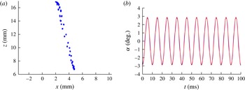
) to the laser beam when the film is at rest. When the system oscillates, the spot produced by the laser moves across the sensor, by three different mechanisms: (1) L moves in the vertical direction, due to the combined movements of the Plateau border and the film; (2) as the film moves in the vertical direction, it intersects the laser at a different spot (L moves along the radius of the film); and (3) the local slope of the film changes and deflects the laser from its original direction. In our experiments, the last effect is always dominant (the first two effects are approximately ten times weaker), and simple geometry allows us to correlate the position of the laser spot on the sensor to the local slope of the film in L. Given the range of excitation forcing frequencies tested in this work, the film features an axisymmetric deformation. We have checked that more complex, non-axisymmetric patterns, such as the ones shown in Couder et al. (Reference Couder, Chomaz and Rabaud1989), Afenchenko et al. (Reference Afenchenko, Ezersky, Kiyashko, Rabinovich and Weidman1998), Vega et al. (Reference Vega, Higuera and Weidman1998) and Elias et al. (Reference Elias, Hutzler and Ferreira2007), appear on the film only above 200 Hz. This allows us to deduce, from this measure of a local slope, the entire profile; see (3.16) for the predicted axisymmetric profile. Moreover, to simplify the analysis of the data, we ideally want the direction of the laser and the radius of the film containing L to be in the same plane (see figure 5), so that the laser beam moves only in a vertical plane after it has been reflected off the film. We show in figure 6(a) a typical result of the tracking of the laser spot on the sensor; in practice its movement follows not a strict line but rather a tilted ellipse. We have checked that both the tilt and the eccentricity are quantitatively compatible with slight misalignments of the system (namely that the plane containing the incident laser beam is slightly off the centre of the suspended film). We therefore use only the vertical position of the spot to determine the local (axisymmetric) slope of the film in L.
Observation of the film in a forced oscillation experiment with
 $f=100$
Hz, a sound amplitude of 90 dB and
 $s_{P}=0.48~\text{mm}^{2}$
. (a) Successive positions of the laser spot on the sensor of the high-speed camera (
 $x$
and
 $y$
are coordinates on the sensor itself, with
 $y$
running in the vertical direction). (b) Local slope of the film in L as a function of time; the time base is the same as in figure 7. The solid line is a sinusoidal fit of the form
 $z=z_{0}+A\cos (2{\rm\pi}ft+{\it\phi})$
, with amplitude
 $A=2.9^{\circ }$
and phase
 ${\it\phi}=3.12$
rad. For clarity, only a portion of the data is plotted (the entire set is 1.4 s long).

Alternatively, we performed a series of qualitative observations of the film, without measuring its deflection. Instead, we used a (expanded) laser beam to generate an interference pattern on the entire film, which we imaged with a high-speed camera. This helped to ensure that the thickness of the film remains constant throughout the experiment. In fact, redistribution of the liquid within the film (self-adaptation) does occur at certain forcing frequencies, as previously observed by Boudaoud et al. (Reference Boudaoud, Couder and Ben Amar1999), but over longer time scales than the duration of this experiment (which typically lasts 0.5 s, starting 1–2 s after the speaker has been turned on).
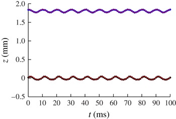
Figure 7 shows a typical result for the movement of the Plateau border. Both its boundaries oscillate sinusoidally with a fixed amplitude, at the forcing frequency
 $f$
. Sinusoidal fits allow us to extract this amplitude, as well as the phase of these oscillations. Their amplitudes and phases, however, may differ slightly (as seen in this particular example). This is a signature of complex deformations of Plateau borders; in such cases, the Plateau border is not simply translated as a whole, and analysis of the experimental movies reveals waves travelling along the Plateau border. However, the amplitude of these deformations (typically 0.1 mm) is smaller than the vertical translation of the Plateau border.
Vertical positions of the upper and lower boundaries of the Plateau border in a forced oscillation experiment with
 $f=100$
Hz, a sound amplitude of 90 dB and
 $s_{P}=0.48~\text{mm}^{2}$
. Solid lines represent sinusoidal fits of the form
 $z=z_{0}+A\cos (2{\rm\pi}ft+{\it\phi})$
, with amplitudes
 $A_{sup}=0.042~\text{mm}$
and
 $A_{inf}=0.046~\text{mm}$
, and with phases
 ${\it\phi}_{sup}=2.93$
rad and
 ${\it\phi}_{inf}=2.04$
rad; notice the significant phase difference
 ${\it\phi}_{sup}-{\it\phi}_{inf}$
. For clarity, only a portion of the data is plotted (the entire set is 1.4 s long).

Figure 6(b) shows the corresponding data for the film, i.e. its local slope at point L, where the laser beam is reflected. Exactly like the Plateau border, the film oscillates with a given amplitude at the forcing frequency
 $f$
, and fitting provides both its amplitude and its phase (with the same time base as the Plateau border). Given the diameter of the film and the position of L, the maximum deflection
 $z_{f}$
of the film (at its centre, in the reference frame of the Plateau border) is then proportional to the slope that we measure:
 $z_{f}~\text{(mm)}\approx 0.16\,{\it\alpha}$
(deg.).
4.2. Results
Presenting the frequency-dependent amplitude of the forced oscillations of the Plateau border and the suspended film, and analysing these data, is not straightforward. Indeed, the coupling between the film and the Plateau border, and hence the result of the experiments, depends strongly on the cross-sectional area of the Plateau border. Ideally, one would use the same three-film system to test a variety of forcing frequencies, to keep both the film and the Plateau border exactly the same, but in practice this is impossible to achieve, due the short lifetime of the films. Instead, each freshly prepared system is subjected to a single forcing frequency. An additional difficulty is then that the cross-sectional area of the Plateau border is impossible to control exactly (the thickness of the film also varies between experiments, up to a factor of three, but as mentioned earlier its mass is small compared to the added mass of the air, and we expect no significant effect associated with this variation). In fact, the cross-sectional areas of the Plateau borders are distributed fairly homogeneously across their entire range (the distribution is similar to that of the data in figure 3 a).
To simplify the representation of the data, we divide our experiments, somewhat arbitrarily, into two categories: those with ‘large’ Plateau borders (where
 $s_{P}>0.3$
mm
 $^{2}$
, with an average of
 $\langle s_{P}\rangle =0.48$
mm
 $^{2}$
and a standard deviation of 0.11 mm
 $^{2}$
) and those with ‘small’ Plateau borders (
 $s_{P}<0.2$
mm
 $^{2}$
, with an average of
 $\langle s_{P}\rangle =0.11$
mm
 $^{2}$
and a standard deviation of 0.07 mm
 $^{2}$
). This categorisation also corresponds, loosely speaking, to a separation between weak and strong coupling between the films and the Plateau border, respectively for large and small Plateau borders (see § 3).
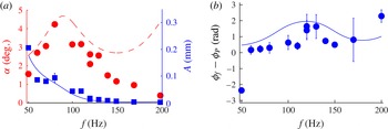
Starting with the case of large Plateau borders, we show in figure 8(a) the response of the film and of the Plateau border as a function of the forcing frequency. The response of the film is typical of a resonance: it shows a maximum at 90 Hz, with a 3 dB bandwidth between 50 and 130 Hz. The amplitude of the Plateau border is a decreasing function of the forcing frequency, with a small hump around 90 Hz. The phase difference between the film and the Plateau border is displayed on figure 8(b); except at 50 Hz, it is positive, and increases from 0 to 2 rad between 60 and 200 Hz.
(a) Amplitude of the film (maximum angle
 ${\it\alpha}$
at point L, circles) and of the Plateau border,
 $A$
(squares) as a function of the forcing frequency, for
 $h=4.8~\text{mm}$
, a forcing amplitude of 90 dB and a cross-section larger than 0.3 mm
 $^{2}$
. Lines are fitted by the model (5.7)–(5.9), with
 $\bar{{\it\lambda}}=0.4$
: the plain curve is the prediction for
 $|\hat{Z}|$
and the dashed curve for
 $|{\it\zeta}|$
. The lowest forcing frequency (50 Hz) is very close to the resonant frequency of our set-up, so the corresponding data might be considered an artefact. (b) Corresponding phase difference between the film and the Plateau border; the solid line is the prediction of the model.

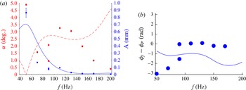
The case of small Plateau borders is shown in figure 9, and the response of the system is qualitatively different from that in figure 8(a). A resonance peak still appears, at a forcing frequency of 110 Hz, which is slightly higher than before; but now the amplitude of the film decreases with the forcing frequency in the range 50–90 Hz. The amplitude of the Plateau border is still a decreasing function of the forcing frequency, again with a small hump at 110 Hz.
(a) Amplitude of the film (maximum angle
 ${\it\alpha}$
at point L, circles) and of the Plateau border,
 $A$
(squares) as a function of the forcing frequency, for
 $h=4.8~\text{mm}$
, a forcing amplitude of 90 dB and a cross-section smaller than 0.3 mm
 $^{2}$
. Lines are fitted by the model (5.7)–(5.9), with
 $\bar{{\it\lambda}}=0.4$
obtained from fitting ‘large’ Plateau borders: the plain curve is the prediction for
 $|\hat{Z}|$
and the dashed curve for
 $|{\it\zeta}|$
. (b) Corresponding phase difference between the film and the Plateau border; the solid line is the prediction of the model.

Qualitatively, these results fit with the picture of coupled oscillations. To elaborate, for large Plateau borders, the resonance frequency of the film and the fundamental eigenfrequency of the Plateau border are well separated (the latter is below 30 Hz for
 $s_{P}>0.3$
mm
 $^{2}$
; see figure 3
a), and hence the resonance of the film is not influenced much by the dynamics of the Plateau border. For small Plateau borders, however, these two frequencies are closer, and the film and the Plateau border may display a stronger interaction for forcing frequencies between the two eigenfrequencies, which may result in a different response of the system. We develop this idea in the next section, by adapting our model of § 3 to the case of forced oscillations.
5. Forced oscillations: modelling
5.1. Resonance frequency of the suspended film
The model of § 3 can already predict the resonance frequency of the film. Equation (3.16) shows that the amplitude of the film has singularities when
 $qa$
(or
 ${\it\omega}/{\it\omega}_{f}$
) is a zero of
 $\text{J}_{0}$
. The lowest positive root of
 $\text{J}_{0}$
is approximately 2.405, so the lowest resonance frequency of the film is
 $2.405{\it\omega}_{f}/(2{\rm\pi})$
, where
 ${\it\omega}_{f}$
is given by (3.15). This gives a value of 103 Hz, in good agreement with the measured resonance frequency (figures 8
a and 9, respectively 90 Hz and 110 Hz). Such good agreement is remarkable (and perhaps fortuitous), because this eigenfrequency depends crucially on the air inertia, which we modelled quite crudely as the added mass of a rigid disk in § 3.3. It does confirm, however, the validity and robustness of the assumptions made.
5.2. Coupled dynamics and forcing
We now include the effect of the forcing sound waves in our model. Since the speed of sound in air is 340 m s
 $^{-1}$
and the highest forcing frequency is 200 Hz, the acoustic wavelength is at least 1.7 m in our experiments, much larger than the size of the system; hence air flow around the films can be taken as incompressible. For simplicity, we further assume that the pressure is uniform on each side of the suspended film, and we denote the pressure difference between the lower and upper sides by
 ${\rm\Delta}P(t)={\rm\Delta}P_{0}\cos {\it\omega}t$
. This disregards the complexity of the pressure field around the system; however, our goal is not to solve the complicated air flow around the films, but to model the acoustic forcing as simply as possible. We keep assumption (5) of § 3.1, which implies that we should neglect the influence of the pressure difference on the suspending films. We also neglect its influence on the Plateau border, which is consistent with the assumption that
 $s_{P}\ll a^{2}$
. Hence, in the right-hand side of the force balance (3.8) for the portion of film between
 $r$
and
 $r+\text{d}r$
, we insert the additional term
 $2{\rm\pi}r\,{\rm\Delta}P(t)\,\text{d}r$
, while the force balance of the Plateau border (3.5) is unaffected.
However, the resonant curves of figures 8(a) and 9 show that the damping cannot be neglected in predicting the response of the system; this is the only assumption of our model that we need to reconsider. Because we could not determine the real source of the dissipation in our system, we chose the simplest possible form and used a simple linear damping force proportional to the vertical velocity of the film,
 $\partial _{t}z(r,t)$
; therefore, in the right-hand side of (3.8) we insert a term
 $-2{\rm\pi}r\,\text{d}r\times {\it\lambda}\partial _{t}z$
, where
 ${\it\lambda}$
is a phenomenological damping coefficient. With this damping term and the pressure contribution, (3.8) becomes
 $$\begin{eqnarray}\left(2{\rm\pi}{\it\rho}er\,\text{d}r+{\textstyle \frac{16}{3}}{\it\rho}_{a}ar\,\text{d}r\right)\partial _{tt}z=4{\rm\pi}{\it\sigma}\partial _{r}(r\partial _{r}z)\,\text{d}r+2{\rm\pi}r\,{\rm\Delta}P(t)\,\text{d}r-2{\rm\pi}{\it\lambda}r\partial _{t}z\,\text{d}r,\end{eqnarray}$$
and (3.9) becomes
 $$\begin{eqnarray}\frac{1}{r}\partial _{r}(r\partial _{r}z)+\frac{{\rm\Delta}P(t)}{2{\it\sigma}}-\frac{{\it\lambda}}{2{\it\sigma}}\partial _{t}z=\frac{1}{2{\it\sigma}}\left({\it\rho}e+\frac{8}{3{\rm\pi}}{\it\rho}_{a}a\right)\partial _{tt}z.\end{eqnarray}$$
Therefore, writing
 $z(r,t)=\text{Re}\,[\hat{z}(r)\text{e}^{-\text{i}{\it\omega}t}]$
and
 $Z(t)=\text{Re}\,(\hat{Z}\text{e}^{-\text{i}{\it\omega}t})$
, instead of (3.13) we have
 $$\begin{eqnarray}\frac{1}{r}\frac{\text{d}}{\text{d}r}\left(r\frac{\text{d}\hat{z}}{\text{d}r}\right)+q_{{\it\lambda}}^{2}\hat{z}=\frac{{\rm\Delta}P_{0}}{2{\it\sigma}},\end{eqnarray}$$
where
 $q_{{\it\lambda}}^{2}=q^{2}(1-\text{i}\bar{{\it\lambda}})$
with the dimensionless film damping coefficient
 $\bar{{\it\lambda}}={\it\lambda}{\it\omega}/2{\it\sigma}q^{2}$
, while the boundary conditions (3.10) and (3.11) give
 $\text{d}_{r}\hat{z}(0)=0$
and
 $\hat{z}(a)=\hat{Z}$
. Solving (5.3) gives
 $$\begin{eqnarray}\hat{z}=A\text{J}_{0}(q_{{\it\lambda}}r)+\frac{{\rm\Delta}P_{0}}{2{\it\sigma}q_{{\it\lambda}}^{2}}.\end{eqnarray}$$
Hence, if we quantify the film deformation by the length
 ${\it\zeta}=\hat{z}(0)-\hat{Z}$
(the maximum deflection of the film in the frame of the Plateau border), we have
 $$\begin{eqnarray}\hat{z}(r)=\hat{Z}+\frac{\text{J}_{0}(q_{{\it\lambda}}r)-\text{J}_{0}(q_{{\it\lambda}}a)}{1-\text{J}_{0}(q_{{\it\lambda}}a)}{\it\zeta}\end{eqnarray}$$
and hence
 $$\begin{eqnarray}\frac{\text{d}\hat{z}}{\text{d}r}=\frac{q_{{\it\lambda}}\text{J}_{1}(q_{{\it\lambda}}r)}{1-\text{J}_{0}(q_{{\it\lambda}}a)}{\it\zeta},\end{eqnarray}$$
showing that the slope of the film is proportional to
 ${\it\zeta}$
and independent of the motion of the Plateau border, which is convenient for comparing with the experiments. Substituting (5.5) into (5.3), we get
 $$\begin{eqnarray}\hat{Z}-\frac{\text{J}_{0}(q_{{\it\lambda}}a)}{1-\text{J}_{0}(q_{{\it\lambda}}a)}{\it\zeta}=\frac{{\rm\Delta}P_{0}}{2{\it\sigma}q_{{\it\lambda}}^{2}}.\end{eqnarray}$$
From (5.6), we compute
 $$\begin{eqnarray}\text{d}_{r}\hat{z}(a)=\frac{q_{{\it\lambda}}\text{J}_{1}(q_{{\it\lambda}}a){\it\zeta}}{1-\text{J}_{0}(q_{{\it\lambda}}a)}.\end{eqnarray}$$
Substituting this into (3.5) and using the definition (3.20) of
 ${\it\omega}_{P}$
gives
 $$\begin{eqnarray}(-{\it\omega}^{2}+{\it\Omega}_{P}^{2})\hat{Z}=-{\it\omega}_{P}^{2}\frac{q_{{\it\lambda}}a\text{J}_{1}(q_{{\it\lambda}}a)}{1-\text{J}_{0}(q_{{\it\lambda}}a)}{\it\zeta}.\end{eqnarray}$$
The solution of the linear system of (5.7) and (5.9) provides a prediction of the forced coupled oscillations: the amplitude of the Plateau border oscillations is
 $|\hat{Z}|$
; the slope of the film is proportional to
 $|{\it\zeta}|$
; and the phase difference between the film and the Plateau border is
 $\arg {\it\zeta}-\arg \hat{Z}$
. In figure 8 we compare the predictions of the model and the experimental results for large Plateau borders, up to a constant prefactor, treating the dimensionless film damping coefficient as a fitting parameter, and using as an input the average cross-sectional area
 $\langle s_{P}\rangle =0.48$
mm
 $^{2}$
. Concerning the amplitudes, good agreement is found for a damping coefficient of
 $\bar{{\it\lambda}}=0.4$
(figure 8
a). The model predicts very well the position of the resonance. Notice that the resonance frequency is not a fitting parameter. The agreement between the experiment and the model is close for the phase difference (figure 8
b). This confirms that our model of the masses and stiffnesses involved in the system is quite satisfactory.
On the other hand, our simple model breaks down above 150 Hz, where it predicts the wrong variation for the amplitude of the film oscillations. The most probable cause of this discrepancy is the simplistic dissipative term; a tailored (and arbitrary) dissipation that increases with the forcing frequency, i.e. a dispersive dissipation (e.g. with a frequency-dependent damping coefficient
 ${\it\lambda}$
of the form
 ${\it\lambda}\propto {\it\omega}^{2}$
), does allow us to practically collapse our model to the high-forcing-frequency part of the data, while maintaining a good fit around the resonance. Another possible reason for this discrepancy is that assumption (4) made in § 3.1, of a rigid Plateau border, breaks down in this range of forcing frequencies. Indeed, as already mentioned in § 4.1, the Plateau border displays strong deformations, with a significant phase difference between its upper and lower boundaries that increases at increasing forcing frequency (data not shown). This echoes recent observations of strong Plateau border distortions with modulations of cross-sections (Elias et al.
Reference Elias, Janiaud, Bacri and Andreotti2014; Cohen et al.
Reference Cohen, Fraysse, Rajchenbach, Argentina, Bouret and Raufaste2014).
We now compare the experiments and the model for small Plateau borders, using as input the average cross-sectional area
 $\langle s_{P}\rangle =0.11$
mm
 $^{2}$
and
 $\bar{{\it\lambda}}=0.4$
. The agreement on the amplitudes is only qualitative (figure 9): the model does reproduce the strong coupling, with a double resonance peak for the film amplitude, but the first peak is seen at forcing frequencies significantly lower than those observed in experiments. Note that the comparison is more difficult to make in this case, because the values of
 $s_{P}$
are more dispersed (the ratio of the standard deviation to the mean of
 $s_{P}$
is 59 % for these small Plateau borders, whereas it is only 22 % for the large ones).
As in the case of free oscillations, we were not able to pinpoint with certainty the source of the dissipative term. Among the different possibilities that we explored, the most relevant is the viscous dissipation in the air that is displaced by the film. To estimate it, we represented the film by a disk of radius
 $a$
, consistent with our estimate for the added mass of the film (details are given in § A.2). However, the predicted damping is around five times smaller than what is observed experimentally. This may be due to the crudeness of our approximation, or to the fact that another source of dissipation is dominant. We have also checked that in the range of forcing frequencies of the forced oscillation experiments, the damping of the Plateau border, which could be added as a term proportional to
 ${\dot{Z}}$
in the left-hand side of (3.5), has no significant influence; so we simply discard it.
6. Conclusions
In summary, we have studied the vibration properties of a suspended film bounded by a Plateau border. In free oscillations experiments, we showed that the eigenfrequency of the system varies with the cross-sectional area of the Plateau border and the geometry of the suspending films. A simplified model allowed us to predict this eigenfrequency with no adjustable parameters. Most notably, it showed that the coupling between the film and the Plateau border has to be taken into account to fully reproduce the experimental data: even in these slow oscillations, the film is not passively transported by the Plateau border.
The coupling is even more apparent in forced oscillations, and it can be seen in the amplitudes of oscillations of the film and of the Plateau border, as well as in their phase difference. In particular, for small Plateau borders the resonant response of the system is qualitatively different than that for larger Plateau borders, due to a stronger influence of the film. We reproduced this behaviour by extending the model used for free oscillations.
In both situations, we could not pinpoint with certainty the main source of dissipation. In the case of free oscillations, we showed experimentally that the damping ratio does not depend on the shear viscosity of the solution. In the case of forced oscillations (which occur at higher forcing frequencies), we showed that viscous dissipation in the air is not negligible anymore, but our estimates seem to show that it remains significantly smaller than the observed damping. Other sources of dissipation are possible, such as the unsteady flow in the transition regions, the flow within the Plateau border induced by its deformation and surface dissipation. However, the study of these possible contributions is beyond the scope of this work, since they pose fundamental questions that are probably better investigated in simpler geometries. Future work will need to address this issue, which is of particular fundamental and practical interest.
Finally, it is worth mentioning that the model used to explain our measurements is close to the one proposed by Pierre et al. (Reference Pierre, Dollet and Leroy2014) to rationalise acoustic propagation through foams, which reinforces the idea of a key ingredient underlying the high-frequency dynamics of foams: the coupled vibration of films and Plateau borders. The main difference lies in the treatment of the surrounding air, which is enclosed in bubbles within the foam but is free to recirculate around the films in our open system. In this respect, accounting for the role of air may be simpler in larger systems and/or for higher forcing frequencies, where the soap films exhibit several modes to which air dynamics is slaved (Kosgodagan Acharige et al. Reference Kosgodagan Acharige, Elias and Derec2014). Such systems, e.g. long Plateau borders (Elias et al. Reference Elias, Kaurin, Arbogast, Leroy, Gay and Derec2015), are thus complementary to our set-up and can probably shed further light on the vibrational response of liquid foams.
Acknowledgements
We thank F. Elias, C. Derec, C. Gay, V. Leroy and I. Cantat for their insightful comments. J.P. and B.D. acknowledge support from Agence Nationale de la Recherche (ANR-11-BS09-001-Samousse) and thank all the members of this ANR consortium coordinated by F. Elias for helpful discussions. J.S. acknowledges support from Région Bretagne (CREATE MOUSPORE) and Agence Nationale de la Recherche (ANR-13-PDOC-0014-01-HydroSurfDyn).
Appendix A. Discussion of damping
In this appendix, we give a few details on the different sources of dissipation that we considered. As mentioned in the main text, unfortunately none of these sources were fully compatible with our experimental results; however, we believe that they may be dominant in other configurations (for systems of larger or smaller length scales, for example). In § A.1 we consider the dissipation that arises as films are extracted from and pulled into the Plateau border. In § A.2 we discuss the dissipation due to movement of the air surrounding the film.
A.1. Dissipation in the Plateau border region
Here we discuss one possible source of dissipation for the oscillations of the Plateau border, namely the viscous flow in the transition regions between the films and the Plateau border. We will recall how to compute this flow, and show that one consequence of this flow is a velocity-dependent modification of the surface tension of the upper and lower suspending films. We will show that this modification amounts to including a dissipative force in the equation of motion of the Plateau border, leading to a damping coefficient of the same order of magnitude as the experimental one, but with an incorrect scaling in viscosity.
A.1.1. Velocity dependence of the traction force of a film on a Plateau border
It is known that the traction force of a film on the Plateau border depends on the relative motion of the film and the Plateau border (Seiwert, Dollet & Cantat Reference Seiwert, Dollet and Cantat2014). If a film is pulled from a reservoir (here, the Plateau border), its traction is greater than twice the equilibrium surface tension, in response to the flow generated in a transition region between the reservoir and the film. This increase depends crucially on the interfacial viscoelasticity (Denkov et al. Reference Denkov, Subramanian, Gurovich and Lips2005) and on the ability of surfactants to adsorb, desorb and diffuse in the bulk and along the interface (Levich Reference Levich1962). A classical assumption is incompressibility of the interface, whereby the surface velocity equals the pulling velocity; this leads to so-called Frankel’s law, which determines uniquely the soap film thickness as a function of the pulling velocity (Mysels, Shinoda & Frankel Reference Mysels, Shinoda and Frankel1959), and in the framework of this hypothesis it is easy to derive the increase in surface tension.
However, such an approach is questionable in the context of our experiments, for three reasons. (i) During the oscillations, the films are alternately withdrawn from and plunged into the Plateau border. In contrast to the pulling situation, there is not a unique relationship between the plunging velocity and the film thickness. However, since we are concerned with oscillations, the films that are plunging into the Plateau border were previously withdrawn from it (with the exception of the first oscillation); hence it may be assumed that at all times, the portion of the film that is successively withdrawing from and plunging into the Plateau border has a thickness given by Frankel’s law. This hypothesis allows us to derive the decrease in surface tension during plunging phases, and is at the basis of the ‘laid-down’ film region proposed by Schwartz & Princen (Reference Schwartz and Princen1987) to model the effective viscosity of foams and emulsions. (ii) Frankel’s law relies on a steady calculation of the transition region, which is doomed to failure at high enough frequencies. (iii) The three transition regions between the Plateau border and the three films may not be treated as independent, and may interact through the Plateau border.
Assuming that we can apply the quasi-steady condition and neglect the coupling between different transition regions, here we review how to derive the velocity dependence of the surface tension of a film pulled at velocity
 $U$
from a Plateau border; see Cantat (Reference Cantat2013) for further details. The derivation follows closely that of Frankel’s law (Mysels et al.
Reference Mysels, Shinoda and Frankel1959) and is also very similar to the Landau–Levich problem of plate coating (Landau & Levich Reference Landau and Levich1942) and the description of motion of a bubble in a tube (Bretherton Reference Bretherton1961). We focus on the transition region between the Plateau border of radius
 $R$
and the flat film, of thickness
 $2h_{\infty }$
. This region has a typical extent of
 $\ell \approx h_{\infty }Ca^{-1/3}$
, where
 $Ca={\it\eta}U/{\it\sigma}$
is the capillary number, which allows to use the lubrication approximation
 $\ell \gg h_{\infty }$
provided that
 $Ca^{1/3}\ll 1$
, a condition that is generally met in practice. The continuity of tangential stress at the air/liquid interface then imposes the condition that
 $\text{d}_{x}{\it\sigma}={\it\eta}\partial _{y}v_{x}|_{y=h(x)}$
, with
 $x$
being the coordinate along the film and
 $y$
the coordinate across it. The flow is driven by the gradient of Laplace pressure,
 $\partial _{x}p\simeq {\it\sigma}\,\text{d}_{xxx}h$
, which gives
 $V_{X}(X,Y)=V_{X}(X,H)+h_{\infty }^{2}(Y^{2}-H^{2})\partial _{x}p/(2\ell ^{2})$
with
 $V_{X}=v_{x}/U$
,
 $X=x/\ell$
,
 $Y=y/h_{\infty }$
and
 $H=h/h_{\infty }$
. Assuming that the interface is incompressible, we have
 $V_{X}(X,H)=1$
. Hence, mass conservation dictates that the flux
 $Q=\int _{0}^{H}V_{X}\,\text{d}Y={\it\varepsilon}^{3}H^{3}\,\text{d}_{XXX}H/Ca+H$
, with
 ${\it\varepsilon}=h_{\infty }/\ell$
, is constant and equal to 1 upon applying the boundary conditions
 $V_{X}\rightarrow 1$
and
 $H\rightarrow 1$
as
 $X\rightarrow \infty$
. This yields
 $\text{d}_{x}{\it\sigma}=3{\it\eta}U(H-1)/(h_{\infty }H^{2})$
. Setting
 ${\it\varepsilon}=(3Ca)^{1/3}$
and assuming that the surface tension in the Plateau border retains its equilibrium value, we get
 $$\begin{eqnarray}{\it\sigma}(X\rightarrow \infty )-{\it\sigma}={\it\sigma}(3Ca)^{1/3}\int _{-\infty }^{\infty }\frac{H-1}{H^{2}}\,\text{d}X,\end{eqnarray}$$
where
 $H$
is the solution of
 $\text{d}_{XXX}H=(1-H)/H^{3}$
satisfying the boundary conditions
 $H\rightarrow 1$
and
 $H^{\prime },H^{\prime \prime }\rightarrow 0$
as
 $X\rightarrow \infty$
, which is determined numerically by a shooting method; this gives
 $\int _{-\infty }^{\infty }[(H-1)/H^{2}]\,\text{d}X=1.86$
. Hence, the traction of a film pulled at velocity
 $U$
from a reservoir is
 $$\begin{eqnarray}2{\it\sigma}_{pull}=2{\it\sigma}+3.87{\it\sigma}Ca^{2/3}.\end{eqnarray}$$
Let us now discuss the velocity dependence of the surface tension in the closely related case of a film plunging into the Plateau border at velocity
 $U$
. The boundary condition for the velocity then becomes
 $V_{X}(X,H)=-1$
. Mass conservation leads to a slightly different equation,
 $\text{d}_{XXX}H=(H-1)/H^{3}$
, and we now get
 $\text{d}_{x}{\it\sigma}=-3{\it\eta}U(H-1)/(h_{\infty }H^{2})$
. Linearising the differential equation for
 $H$
about the boundary condition
 $H\rightarrow 1$
as
 $X\rightarrow \infty$
, i.e.
 $H=1+{\it\varepsilon}_{H}$
, gives
 $\text{d}_{XXX}{\it\varepsilon}_{H}={\it\varepsilon}_{H}$
. The general solution that is compatible with the boundary condition is
 ${\it\varepsilon}_{H}=\text{e}^{-X/2}\cos (X\sqrt{3}/2+{\it\phi})$
, up to a numerical prefactor which does not modify the solution. Solving the differential equation by shooting towards decreasing values of
 $X$
from this linearised form gives a limiting value for
 $\text{d}_{XX}H(X\rightarrow -\infty )$
that depends on the value of
 ${\it\phi}$
. As stated before, to guarantee that the thickness of the plunging film is the same as that of the withdrawn film, we choose
 ${\it\phi}$
such that this limiting value equals the one obtained for the pulling case, which turns out to be
 $\text{d}_{XX}H(X\rightarrow -\infty )=0.643$
. This fixes
 ${\it\phi}=1.156$
, and the numerical resolution then gives
 $\int _{-\infty }^{\infty }[(H-1)/H^{2}]\,\text{d}X=0.55$
. Hence, the traction of a film pushed at velocity
 $U$
into a reservoir is
 $$\begin{eqnarray}2{\it\sigma}_{push}=2{\it\sigma}-1.15{\it\sigma}Ca^{2/3}.\end{eqnarray}$$
A.1.2. Damping from the dissipation in the transition regions between the films and the Plateau border
If the Plateau border is moving upwards (
 ${\dot{Z}}>0$
), the magnitude of the force
 $f_{+}=2{\it\sigma}_{+}$
exerted by the upper suspending film decreases, whereas that of the lower suspending film,
 $f_{-}=2{\it\sigma}_{-}$
, increases, compared to the equilibrium surface tension. The situation is reversed when the Plateau border is moving downwards (
 ${\dot{Z}}<0$
). We now show that this results in a friction force against the motion of the Plateau border. At leading order in
 $Z/h$
, the velocity of the suspended film with respect to the Plateau border is negligible compared to the velocities of the suspending films, so we will assume that its surface tension does not vary. Combining (A 2), (A 3) and (3.1), we get
 $$\begin{eqnarray}\frac{{\it\mu}}{2{\it\sigma}}\ddot{Z}=-[1+f({\dot{Z}})Ca_{{\dot{Z}}}^{2/3}]\left(\frac{\sqrt{3}}{2}+\frac{\sqrt{3}}{4}\frac{Z}{h}\right)+[1+f(-{\dot{Z}})Ca_{{\dot{Z}}}^{2/3}]\left(\frac{\sqrt{3}}{2}-\frac{\sqrt{3}}{4}\frac{Z}{h}\right),\end{eqnarray}$$
where
 $f({\dot{Z}})=1.94$
if
 ${\dot{Z}}>0$
and 0.58 if
 ${\dot{Z}}<0$
and where
 $Ca_{{\dot{Z}}}={\it\eta}|{\dot{Z}}|\sqrt{3}/2{\it\sigma}$
is the capillary number based on the relative velocity
 $|{\dot{Z}}|\sqrt{3}/2$
(at leading order in
 $Z/h$
) of the Plateau border and the suspending films. We have
 $f(-{\dot{Z}})-f({\dot{Z}})=2.52\,\text{sign}({\dot{Z}})$
, so we can rewrite the equation of motion as
 $$\begin{eqnarray}\frac{{\it\mu}}{2{\it\sigma}}\ddot{Z}+\frac{\sqrt{3}}{2}2.52\text{sign}({\dot{Z}})\left(\frac{{\it\eta}|{\dot{Z}}|\sqrt{3}}{2{\it\sigma}}\right)^{2/3}+\frac{\sqrt{3}}{2}\frac{Z}{h}=0.\end{eqnarray}$$
This is the equation of an oscillator with nonlinear damping, coming from the variations of surface tension due to the viscous flow in the transition region between the films and the Plateau border. With
 $\bar{t}={\it\omega}_{0}t$
and
 $\bar{Z}=Z/h$
, the equation becomes
 $$\begin{eqnarray}\partial _{\bar{t}\,\bar{t}}\bar{Z}+{\it\lambda}|\partial _{\bar{t}}\bar{Z}|^{2/3}\text{sign}(\partial _{\bar{t}}\bar{Z})+\bar{Z}=-\frac{2}{\sqrt{3}}\partial _{r}z(a,t),\end{eqnarray}$$
with a dimensionless damping coefficient
 $$\begin{eqnarray}{\it\lambda}=2.56\frac{\sqrt{3}}{2}\left(\frac{{\it\eta}^{2}h}{{\it\sigma}{\it\mu}}\right)^{1/3}.\end{eqnarray}$$
This damping coefficient is proportional to
 ${\it\eta}^{2/3}$
; hence it increases by factors of 2.8 and 11 when going from a solution without glycerol to a solution containing, respectively, 50 % and 80 % of glycerol. This is not compatible with our experiments, where we showed that the damping coefficient is barely dependent on the glycerol concentration (figure 3
b) and hence on the shear viscosity (table 1). Nonetheless, for the solution without glycerol, taking
 ${\it\sigma}=0.03$
N m
 $^{-1}$
,
 $h=4.8$
mm and
 $s_{P}=0.3$
mm
 $^{2}$
, we find that
 ${\it\lambda}=0.18$
, which is of the same order of magnitude as the experimental values of the damping (figure 3
b). As the viscosity increases, the damping coefficient given by (A 7) overestimates the data.
Hence, one of the two hypotheses made at the beginning of this derivation does not hold in our experiments. It could be that we are not in a quasi-steady situation in the transition region, but we are not aware of any prediction of the transition regions in unsteady oscillatory flow; or there could be some coupling between the different transition regions, but this is a difficult question that deserves a dedicated study, which is beyond the scope of this paper.
A.2. Dissipation in the air
In a thin soap film, the viscous friction in the liquid within the film is usually negligible compared to that of air (Pierre et al.
Reference Pierre, Dollet and Leroy2014; Kosgodagan Acharige et al.
Reference Kosgodagan Acharige, Elias and Derec2014). Therefore, we now perform an estimation of the air friction on the film oscillation at the forcing frequency
 $f$
.
Consistent with assumption (4), the amplitude of oscillation of the film is small compared to its radius. In such a limit, the forces exerted by the air on the oscillating film can be deduced from the unsteady Stokes equations for the air flow (Landau & Lifchitz Reference Landau and Lifchitz1994). As in § 3.3, it is a difficult task to solve the equations in our geometry, and we resort to the simple approximation of identifying the film with an oscillating rigid disk in order to get an estimate of air friction. At angular forcing frequency
 ${\it\omega}$
, a frictional Stokes boundary layer entrained by the film motion develops over a thickness of order
 ${\it\delta}_{a}=\sqrt{2{\it\nu}_{a}/{\it\omega}}$
. In our range of forcing frequencies, this thickness is of order 0.1 mm, which is much smaller than the film radius. In this limit
 ${\it\delta}_{a}\ll a$
, Zhang & Stone (Reference Zhang and Stone1998) have proposed an asymptotic expression for the force
 $\boldsymbol{F}$
of a broadside oscillating disk; with a velocity
 $\boldsymbol{U}\cos {\it\omega}t$
, they found that
 $$\begin{eqnarray}\displaystyle \boldsymbol{F} & \simeq & \displaystyle \text{Re}\,\left\{{\it\mu}_{a}a\boldsymbol{U}\left[-16\left(\frac{1}{6}\text{i}\frac{{\it\omega}a^{2}}{{\it\nu}_{a}}+1.32\text{e}^{0.27\text{i}{\rm\pi}}a\sqrt{\frac{{\it\omega}}{{\it\nu}_{a}}}\right)\right]\text{e}^{\text{i}{\it\omega}t}\right\}\nonumber\\ \displaystyle & = & \displaystyle \frac{8}{3}{\it\rho}_{a}a^{3}\frac{\text{d}}{\text{d}t}(\boldsymbol{U}\cos {\it\omega}t)-21.1a^{2}\boldsymbol{U}\sqrt{{\it\mu}_{a}{\it\rho}_{a}{\it\omega}}\cos ({\it\omega}t+0.27{\rm\pi}).\end{eqnarray}$$
In the first term, we recover the added mass force on the disk, already used in § 3.3. The second term gives the friction force. More precisely, it contains a contribution opposite to the velocity and an out-of-phase contribution, giving a small correction to the inertia, which we neglect. Hence, we retain a friction force
 $\boldsymbol{F}_{a}=-21.1\cos (0.27{\rm\pi})\times a^{2}\boldsymbol{U}\sqrt{{\it\mu}_{a}{\it\rho}_{a}{\it\omega}}\cos {\it\omega}t=-14.0a^{2}\boldsymbol{U}\sqrt{{\it\mu}_{a}{\it\rho}_{a}{\it\omega}}\cos {\it\omega}t$
.
As in § 3.3, we assume that the friction is uniformly distributed over the film. Moreover, regarding the air friction of the portion of film between
 $r$
and
 $r+\text{d}r$
, we simply assume that we can replace
 $\boldsymbol{U}\cos {\it\omega}t$
by the local vertical velocity
 $\partial _{t}z(r,t)$
. With these two approximations, the portion of film experiences a friction force of magnitude
 $$\begin{eqnarray}\text{d}f_{a}=\frac{2{\rm\pi}r\,\text{d}r}{{\rm\pi}a^{2}}[-14.0a^{2}\sqrt{{\it\mu}_{a}{\it\rho}_{a}{\it\omega}}\,\partial _{t}z(r,t)]=-2\times 14.0r\sqrt{{\it\mu}_{a}{\it\rho}_{a}{\it\omega}}\,\partial _{t}z(r,t).\end{eqnarray}$$
Identifying this force with the last term in the right-hand side of (5.1), we get, after some algebra, the following expression for
 $\bar{{\it\lambda}}$
in (5.3):
 $$\begin{eqnarray}\bar{{\it\lambda}}=\frac{14.0\sqrt{{\it\mu}_{a}{\it\rho}_{a}/{\it\omega}}}{{\rm\pi}{\it\rho}e+8{\it\rho}_{a}a/3}.\end{eqnarray}$$
In our range of forcing frequencies,
 $f\approx 10^{2}$
Hz, and we get
 $\bar{{\it\lambda}}\approx 0.07$
, which is five times smaller than the experimental value of the damping coefficient that fits the resonance curve,
 $\bar{{\it\lambda}}=0.4$
. Air friction is therefore not negligible, but judging from this estimate it is unlikely to be the only contribution to dissipation.