2.1. The GK equations

The starting point for our derivation is given by the GK equations in the presence of a straight magnetic guide field (acting here in the $z$-direction, $B_0\hat {\boldsymbol {z}}$). The community regularly employs the GK equations in the study of kinetic plasma at sub-gyroradius scales ($k_\perp \rho _i > 1$), and we have used them to probe the fundamental nature of GK turbulence (Teaca et al. Reference Teaca, Navarro, Jenko, Brunner and Villard2012; Teaca, Navarro & Jenko Reference Teaca, Navarro and Jenko2014; Teaca, Jenko & Told Reference Teaca, Jenko and Told2017; Teaca et al. Reference Teaca, Navarro, Told, Görler, Plunk, Hatch and Jenko2019, Reference Teaca, Gorbunov, Told, Bañón Navarro and Jenko2021). A simple $\delta f$-derivation of the GK equations for a Maxwellian background distribution function ($F_s$) is presented in Howes et al. (Reference Howes, Cowley, Dorland, Hammett, Quataert and Schekochihin2006) and Schekochihin et al. (Reference Schekochihin, Cowley, Dorland, Hammett, Howes, Quataert and Tatsuno2009) and as such, we do not insist here on the GK construction.

For $h_s = h_s(\boldsymbol {R}_s,v_{\parallel },\mu)$ the non-adiabatic part of the GK distribution function (with the particle perturbed distribution function being found as $\delta f_s= - q_s \phi F_s/T_s + h_s$), we simply list in the following the GK equations in non-dimensional form and in the absence of collisions

(2.1)$$ \frac{\partial h_s}{\partial t}+ \frac{1}{B_0}\{\chi_s, h_s\} + v_{T_s}v_{{\parallel}} \frac{\partial h_s}{\partial z}=\frac{q_s }{T_{s}}F_s\frac{\partial \chi_s}{\partial t}, $$

where $\{\chi _s, h_s\}=(\boldsymbol {\nabla } \chi _s \times \boldsymbol {\nabla } h_s)\boldsymbol {\cdot } \hat {\boldsymbol {z}}$ is the nonlinearity written in term of a Poisson bracket structure, $v_{Ts}=(\sqrt {2T_s/m_s})$ is the thermal velocity for a species $s$ of charge $q_s$, mass $m_s$ and background temperature $T_s$ (all expressed in terms of reference units, see appendix A). The perpendicular velocity dependence is expressed in term of the magnetic moment $\mu$ (in non-dimensional form, $\mu B_0= v_\perp ^2$) and the equilibrium distribution function $F_s$ has the simple form

(2.2)$$ F_s = {\rm \pi}^{{-}3/2}\exp({-{v_\parallel^2}-\mu B_0}). $$

Here, $\chi _s$ is the gyroaveraged GK potential. It is convenient to represent it in Fourier space, as the gyroaverage operations reduce to the multiplication of Bessel functions of zero ($J_0$) and first ($J_1$) order,

(2.3)$$ \chi_s(\boldsymbol{k},\mu,v_\parallel) = \sum_{\boldsymbol{k}} \exp({{\rm i}\boldsymbol{k}\boldsymbol{\cdot}\boldsymbol{R}_s})\left[J_0\left(\lambda_s\right) \left(\phi(\boldsymbol{k})-v_{T_s} v_\parallel A_\parallel(\boldsymbol{k})\right)+ \frac{\mu T_{s}}{q_s}\frac{2 J_1\left(\lambda_s\right)}{\lambda_s}B_\parallel(\boldsymbol{k})\right]. $$

The electrostatic potential ($\phi$), magnetic potential in the parallel direction ($A_\parallel$) and magnetic fluctuation in the parallel direction ($B_{\parallel }$) are obtained in wave space from their respective field equations,

(2.4)$$\begin{gather} \phi(\boldsymbol{k},t) = {\rm \pi}B_0\sum_s q_s n_s \int^{+\infty}_{-\infty}{\rm d} v_\parallel \int_0^{\infty}{\rm d}\mu J_0(\lambda_s)h_s(\boldsymbol{k},v_\parallel,\mu,t)/ \sum_s\frac{q_s^2 n_s}{T_s}, \end{gather}$$

(2.5)$$\begin{gather}A_\parallel(\boldsymbol{k},t) = \frac{{\rm \pi} \beta}{2 k_\perp^2}B_0\sum_s q_s n_s v_{T_s} \int^{+\infty}_{-\infty}{\rm d} v_\parallel v_\parallel \int_0^{\infty}{\rm d}\mu J_0 \left(\lambda_s\right)h_s(\boldsymbol{k},v_\parallel,\mu,t), \end{gather}$$

(2.6)$$\begin{gather}B_\parallel(\boldsymbol{k},t) ={-}\frac{{\rm \pi}\beta}{4}B_0\sum_s m_s n_s v_{T_s}^2 \int^{+\infty}_{-\infty}{\rm d} v_\parallel \int_0^{\infty}{\rm d}\mu\, \mu \frac{2J_1\left(\lambda_s\right)}{\lambda_s}h_s(\boldsymbol{k},v_\parallel,\mu,t), \end{gather}$$

where $\beta =8{\rm \pi} n_{\textrm {ref}} T_{\textrm {ref}}/B_{\textrm {ref}}^{2}$ is defined in terms of the reference temperature $T_{\textrm {ref}}$, density $n_{\textrm {ref}}$ and magnetic intensity $B_{\textrm {ref}}$. We also use

(2.7)$$\begin{gather} \lambda_s = \sqrt{2\mu B_0 b_s}, \end{gather}$$

(2.8)$$\begin{gather}b_s = \left(\frac{k_\perp v_{Ts}}{\sqrt{2}\varOmega_s}\right)^2 =\frac{k^2_\perp \rho_s^2}{2}. \end{gather}$$

From the GK equations, we see that the gyroaverage operations, captured by the Bessel functions, smear $k_\perp$ structures into $\mu$ structures at $k_\perp \rho _i > 1$. In the $k_\perp \rho _i \ll 1$ limit, for which the Bessel functions tend towards one, if no initial $\mu$ structure is present in $h_s$, the GK equations cannot generate subsequent $\mu$ structures and we can integrate over the $\mu$ direction without any loss of information. To see this better, and to integrate $\mu$ in a consistent way, we make use of a Laguerre transform approach.

2.2. Laguerre transform

A recent detailed approach for the use of a Laguerre transform for the GK system can be found in Mandell, Dorland & Landreman (Reference Mandell, Dorland and Landreman2018). Here, we present only the information needed to understand the transformations we employ in our derivation. A notable simplification is that we resume to a constant $B_0$ rather than the more general $B_0(z)$ approach employed by Mandell et al. (Reference Mandell, Dorland and Landreman2018). However, we do not resume to the simpler electrostatic limit, and consider electromagnetic fluctuations in our derivation.

For convenience, we define the Laguerre (basis) functions as

(2.9)$$\begin{gather} \psi^l\left(\mu B_0\right) = ({-}1)^l \,{\rm e}^{-\mu B_0} L_l\left(\mu B_0\right), \end{gather}$$

(2.10)$$\begin{gather}\psi_l\left(\mu B_0\right) = ({-}1)^l L_l\left(\mu B_0\right), \end{gather}$$

where $L_l(x) = ({{\rm e}^x}/{l!})({{\rm d}^l}/{{{\rm d}x}^l})x^l \,{\rm e}^{-x}$ are Laguerre polynomials. The Laguerre functions obey the orthonormality condition,

(2.11)$$ \int_{0}^{+\infty}{\rm d}\mu B_0 \psi^k\psi_l = \delta_{kl}, $$

which results from the orthogonality condition of the Laguerre polynomials $L_l(x)$ around the ${\rm e}^{-x}$ weight function (note that $\psi _l(x) \,{\rm e}^{-x}=\psi ^l(x)$). In our derivation, we also make use of the recurrence relation

(2.12)$$ (l+1)\psi^{l+1} = (\mu B_0-2l-1)\psi^l - l\psi^{l-1}. $$

The decomposition of a function $f(\mu )$ in term of the Laguerre basis $\psi ^l$ is done as

(2.13)$$ f(\mu) = \sum_{l=0}^{\infty} \psi^l\left(\mu B_0\right) \hat{f}_l, $$

with the spectral amplitude $\hat {f}_l$ for the Laguerre modes $l$ being found simply as

(2.14)$$ \hat{f}_l = \int_0^{\infty}{\rm d}\mu B_0 \psi_l f(\mu). $$

The Laguerre transforms given by (2.13) and (2.14) allows us to obtain the GK equations in Laguerre space. Apart from projecting $h_s$, we also need to project $J_0(\lambda _s)$ and $({2}/{\lambda _s}) J_1(\lambda _s)$ onto the Laguerre basis. In the drift kinetic limit, retaining the contribution of the Bessel functions will allow FLR effects to be preserved (Dorland & Hammett Reference Dorland and Hammett1993).

Remembering that $\lambda _s = \sqrt {2\mu B_0 b_s}$, and omitting the species subscript $s$, we write the Bessel functions of order $n$ in terms of the basis $\psi _l$, with the coefficients $\mathcal {J}_{nl}$ obtained via a generating function, i.e.

(2.15)$$ J_n\left(\sqrt{2\mu B_0 b }\right) = \sum_l \psi_l \mathcal{J}_{nl} = \sum_l \psi_l \frac{b^l}{l!}\frac{\partial^l}{\partial b^l} \langle J_n \rangle, $$

where

(2.16)$$ \langle J_n \rangle=\int_0^{\infty} {\rm e}^{-\mu B_0} J_n\left(\sqrt{2\mu B_0 b}\right) B_0 \,{\rm d}\mu. $$

Obtaining the same decomposition for the $({2}/{\lambda _s}) J_1(\lambda _s)$ function requires an extra manipulation. Using the well-known recurrence formula for the Bessel functions, we arrive at the expression

(2.17)$$ \frac{2}{\lambda_s} J_1\left(\lambda_s\right) = J_0\left(\lambda_s\right)+J_2\left(\lambda_s\right) = \sum_l \psi_l \tilde{\mathcal{J}}_{1l}=\sum_l \psi_l \frac{b^l}{l!}\frac{\partial^l}{\partial b^l} \left[\langle J_0 \rangle+\langle J_2 \rangle\right]. $$

The coefficients for the $({2}/{\lambda _s}) J_1(\lambda _s)$ function are labelled as $\tilde {\mathcal {J}}_{1l}$ [the tilde notation is used to distinguish it form the coefficients of $J_1(\lambda _s)$] and we express it via the generating function involving $\langle J_0 \rangle$ and $\langle J_2 \rangle$. From (2.16) we obtain

(2.18)$$\begin{gather} \langle J_0 \rangle = {\rm e}^{{-}b/2}, \end{gather}$$

(2.19)$$\begin{gather}\langle J_2 \rangle ={-}\left(\frac{2}{b}+1\right){\rm e}^{{-}b/2} + \frac{2}{b}, \end{gather}$$

and the coefficients for the Bessel functions of interest are obtained as

(2.20)$$\begin{gather} \mathcal{J}_{0l} = \frac{b^l}{l!}\frac{\partial^l}{\partial b^l} {\rm e}^{{-}b/2} , \end{gather}$$

(2.21)$$\begin{gather}\tilde{\mathcal{J}}_{1l} = \frac{b^l}{l!}\frac{\partial^l}{\partial b^l} \left[\left(1-{\rm e}^{{-}b/2}\right)\frac{2}{b}\right]. \end{gather}$$

Compared with Mandell et al. (Reference Mandell, Dorland and Landreman2018), because we account for electromagnetic fluctuations, we needed to obtain $\tilde {\mathcal {J}}_{1l}$. For clarity, the GK equations in Laguerre space are presented next.

2.3. GK system in Laguerre basis

We start by looking at the field equations in Laguerre basis. For $\phi$, given by (2.4), we use (2.13) for the representation of $h_s$ and (2.15) for the representation of $J_0(\lambda _s)$. We obtain

(2.22)$$\begin{align} \phi(\boldsymbol{k},t) & = {\rm \pi}B_0\sum_s q_s n_s\int^{+\infty}_{-\infty}{\rm d} v_\parallel \int_0^{\infty}{\rm d}\mu \sum_l \psi_l\mathcal{J}_{0l}\sum_j \psi^j \hat{h}_{sj}/\sum_s\frac{q_s^2 n_s}{T_s} \nonumber\\ & = {\rm \pi}\sum_s q_s n_s\int^{+\infty}_{-\infty}{\rm d} v_\parallel \sum_l \mathcal{J}_{0l} \hat{h}_{sl}/\sum_s\frac{q_s^2 n_s}{T_s}, \end{align}$$

where we used the orthogonality condition (2.11) to obtain the second line. The same approach is used for $A_\parallel$, which gives

(2.23)$$ A_\parallel(\boldsymbol{k},t) = \frac{{\rm \pi} \beta}{2 k_\perp^2} \sum_s q_s n_s v_{T_s}\int^{+\infty}_{-\infty}{\rm d} v_\parallel v_\parallel \sum_l \mathcal{J}_{0l} \hat{h}_{sl}. $$

For the $B_\parallel$ field equation, after the Laguerre representation for each contributing function is inserted in the first step, we extract $\mu \psi ^j$ from the recurrence relation (2.12) in the second step and use the orthogonality condition (2.11) in the last step, obtaining

(2.24)$$\begin{align} B_\parallel(\boldsymbol{k},t) & ={-}\frac{{\rm \pi}\beta}{4}B_0\sum_s m_s n_s v_{T_s}^2 \int^{+\infty}_{-\infty}{\rm d} v_\parallel \int_0^{\infty}{\rm d}\mu \mu \sum_l \psi_l \mathcal{\tilde J}_{1l}\sum_j \psi^j\hat h_{sj} \nonumber\\ & ={-}\frac{{\rm \pi}\beta}{4}\sum_s m_s n_s v_{T_s}^2\int^{+\infty}_{-\infty}{\rm d} v_\parallel \int_0^{\infty}{\rm d}\mu \sum_l\psi_l \mathcal{J}_{1,l}\sum_j[(2j+1)\psi^j \nonumber\\ & \quad +j\psi^{j-1}+(j+1)\psi^{j-1}]\hat{h}_{sj} \nonumber\\ & ={-}\frac{{\rm \pi}\beta}{2}\sum_s \frac{n_s T_s}{B_0}\int^{+\infty}_{-\infty}{\rm d} v_\parallel \sum_l \mathcal{J}_{1,l}[(2l+1)\hat{h}_{s,l} +l \hat{h}_{s,l-1}+(l+1)\hat{h}_{s,l+1}] . \end{align}$$

With the electromagnetic potentials and fields determined, to project the GK potential (2.3) onto the Laguerre basis, we need to express the Bessel functions contributions and use again the recurrence relation (2.12) to express $\mu \psi _j$, before employing the orthogonality condition (2.11). The $\hat {\chi }_l$ spectral amplitude gives

(2.25)$$\begin{align} \hat{\chi}_l(\boldsymbol{k}) & = \int_0^{\infty}{\rm d}\mu B_0 \psi^l \left[\left(\phi(\boldsymbol{k})-v_{T_s} v_\parallel A_\parallel(\boldsymbol{k})\right) \sum_j \psi_j J_{0j}+\frac{\mu T_{s}}{q_s}B_\parallel(\boldsymbol{k}) \sum_j \psi_j \tilde{\mathcal{J}}_{1j}\right] \nonumber\\ & = B_0\int_0^{\infty} {\rm d} \mu \psi^l\left(\phi(\boldsymbol{k})-v_{T_s} v_\parallel A_\parallel(\boldsymbol{k})\right)\sum_j \psi_j J_{0j} \nonumber\\ & \quad +\frac{T_s}{q_s B_0} B_\parallel(\boldsymbol{k})\sum_ j\left[(j+1)\psi_{j+1}+(2j+1)\psi_{j}+j\psi_{j-1}\right] \tilde{\mathcal{J}}_{1j}\tilde{\mathcal{J}}_{1l} \nonumber\\ & = \mathcal{J}_{0l}\left(\phi(\boldsymbol{k})-v_{T_s} v_\parallel A_\parallel(\boldsymbol{k})\right) + \frac{T_s}{q_s B_0} B_\parallel(\boldsymbol{k})\left((l+1)\tilde{\mathcal{J}}_{1,l+1}+ (2l+1)\tilde{\mathcal{J}}_{1,l}+l\tilde{\mathcal{J}}_{1,l-1}\right). \end{align}$$

To obtain the GK equation (2.1) on the Laguerre basis, we look at each term independently. We remind the reader that because the Bessel functions are expressed in terms of the basis $\psi _l$, and because the explicit $\mu$ dependence in the $B_\|$ term is handled via a Laguerre polynomials recurrence formula, the Laguerre expansion of $\chi$ occurs in terms of the basis $\psi _l$, i.e. $\chi =\sum _l \psi _l \hat {\chi }_l$. The linear terms are computed in a straightforward manner,

(2.26)$$\begin{gather} \int_0^{\infty} {\rm d} \mu B_0 \psi_l \sum_j \psi^j \frac{\partial \hat{h}_j}{\partial t} = \frac{\partial \hat{h}_l}{\partial t}, \end{gather}$$

(2.27)$$\begin{gather}\int_0^{\infty} {\rm d} \mu B_0 \psi_l \sum_j \psi^j v_{T_s}v_{{\parallel}} \frac{\partial \hat{h}_j}{\partial z} = v_{T_s}v_{{\parallel}}\frac{\partial \hat{h}_l}{\partial z}, \end{gather}$$

(2.28)$$\begin{gather}\int_0^{\infty} {\rm d} \mu B_0 \frac{q_s}{T_s} {\rm \pi}^{{-}3/2} \exp({-v^2_{{\parallel}} - \mu B_0}) \psi_l \sum_n \psi_n \frac{\partial \hat{\chi}_n}{\partial t} = \frac{q_s}{T_s} \frac{{\rm e}^{{-}v^2_{{\parallel}}}}{{\rm \pi}^{3/2}} \frac{\partial \hat{\chi}_l}{\partial t}. \end{gather}$$

The only complication arises from the nonlinear term, which, as presented in Mandell et al. (Reference Mandell, Dorland and Landreman2018), is expressed as a convolution

(2.29)$$ \int_0^{\infty} {\rm d} \mu B_0 \frac{1}{B_0}\psi_l \left\{\sum_n \psi_n \hat{\chi}_n, \sum_\kappa \psi_\kappa \hat{h}_\kappa\right\} = \frac{1}{B_0}\sum_{\kappa = 0}^\infty\sum_{n = |\kappa-l|}^{\kappa+l} \alpha_{l\kappa n} \left\{ \hat{\chi}_n, \hat{h}_\kappa\right\}, $$

where $\alpha _{l\kappa n}$ is a convolution coefficient computed as

(2.30)$$ \alpha_{l\kappa n} = \int_0^{\infty} {\rm d}\mu B_0 \psi_\kappa \psi_n\psi^l = \sum_j \frac{(\kappa+l-j)! 2^{2j-\kappa-l+n}}{(\kappa-j)!(l-j)!(2j-\kappa-l+n)!(\kappa+l-n-j)!}, $$

with the summation limits over $j$ being chosen to ensure that the factorials under the sum remain non-negative. Putting all the terms together, gives the GK equation for a Laguerre mode $l$ as

(2.31)$$ \frac{\partial \hat{h}_l}{\partial t} + \frac{1}{B_0}\sum_{\kappa = 0}^\infty \sum_{n = |\kappa-l|}^{\kappa+l} \alpha_{l\kappa n}\left\{ \hat{\chi}_n, \hat{h}_\kappa\right\} + v_{T_s}v_{{\parallel}} \frac{\partial \hat{h}_l}{\partial z} = \frac{q_s}{T_s} \frac{{\rm e}^{{-}v^2_{{\parallel}}}}{{\rm \pi}^{3/2}} \frac{\partial \hat{\chi}_l}{\partial t}. $$

With the GK equation expressed in Laguerre spectral space, we can now take a drift kinetic long-wavelength limit, while retaining FLR effects. We do this in the next section and obtain the equations of interests.

3.1. Drift-kinetic limit

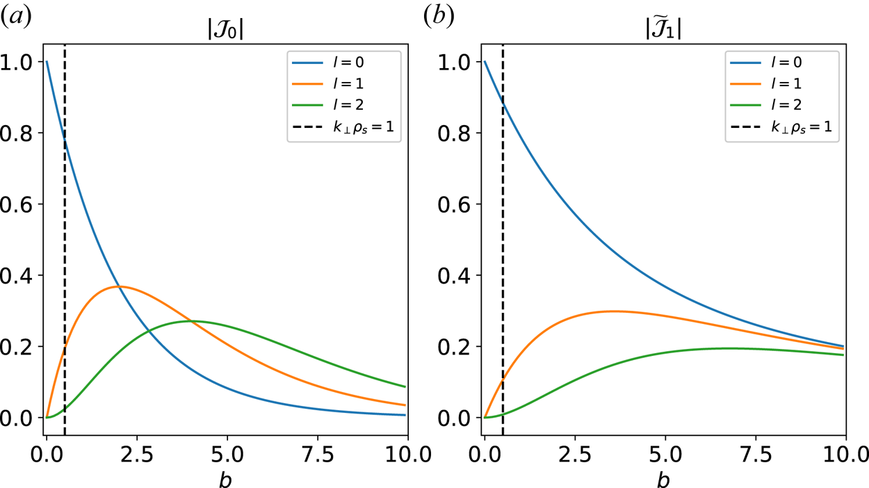
In a drift-kinetic approach, the long-wavelength limit $k_\perp \rho _s\rightarrow 0$ leads to $b_s\rightarrow 0$. Dispensing with the species label, for $b\rightarrow 0$ all $l\ne 0$ terms in (2.20) and (2.21) will tend towards zero (see figure 1). The only non-zero contributions, for $l=0$, are responsible for retaining FLR effects and have the explicit form,

(3.1)$$\begin{gather} \mathcal{J}_{00} = {\rm e}^{{-}b/2}, \end{gather}$$

(3.2)$$\begin{gather}\tilde{\mathcal{J}}_{10} = \left[\left(1-{\rm e}^{{-}b/2}\right)\frac{2}{b}\right]. \end{gather}$$

Figure 1.

Absolute value of moments $\mathcal {J}_{0l}$ and $\tilde {\mathcal {J}}_{1l}$. With $b\rightarrow 0$, all the higher moments approach zero.

We would like to emphasise that we do not make any assumptions on the ratio between of the species’ gyroradii. When this ratio is sufficiently large, one may wish to make further simplifications to the model and potentially neglect FLR effects for the particle species with the smallest gyroradius. However, we consider here the most general case, also applicable to the electron–positron plasma, in addition to the commonly studied proton–electron system. To obtain our equations, which retain the dominant FLR contributions, we set $\mathcal {J}_{0l}=0$ and $\tilde {\mathcal {J}}_{1l}=0$ for all $l>0$ in the GK equations expressed in Laguerre form. By doing so, the field equations (2.22)–(2.24) now give

(3.3)$$\begin{gather} \phi(\boldsymbol{k},t) = {\rm \pi}\sum_s q_s n_s\int^{+\infty}_{-\infty}{\rm d} v_\parallel \mathcal{J}_{00} \hat{h}_{s0}/\sum_s\frac{q_s^2 n_s}{T_s}, \end{gather}$$

(3.4)$$\begin{gather}A_\parallel(\boldsymbol{k},t) = \frac{{\rm \pi} \beta}{2 k_\perp^2}\sum_s q_s n_s v_{T_s} \int^{+\infty}_{-\infty}{\rm d} v_\parallel v_\parallel \mathcal{J}_{00} \hat{h}_{s0}, \end{gather}$$

(3.5)$$\begin{gather}B_\parallel(\boldsymbol{k},t) ={-}\frac{{\rm \pi}\beta}{2}\sum_s \frac{n_s T_s}{B_0}\int^{+\infty}_{-\infty}{\rm d} v_\parallel \tilde{\mathcal{J}}_{10} \left[\hat{h}_{s0} +\hat{h}_{s1} \right]. \end{gather}$$

Looking next at the GK potential and its spectral amplitudes $\hat {\chi }_l$ (2.25), because we set $\mathcal {J}_{0l}=\tilde {\mathcal {J}}_{1l}=0$ for all $l>0$, only $l = 0,1$ contributions remain. We find $\hat \chi _0$ and $\hat {\chi }_1$ to be

(3.6)$$\begin{gather} \hat{\chi}_{0} = \mathcal{J}_{00}\left(\phi(\boldsymbol{k})-v_{T_s} v_\parallel A_\parallel(\boldsymbol{k})\right) + \frac{T_s}{q_s B_0} B_\parallel(\boldsymbol{k})\tilde{\mathcal{J}}_{10}, \end{gather}$$

(3.7)$$\begin{gather}\hat{\chi}_1 = \frac{T_s}{q_s B_0} B_\parallel(\boldsymbol{k}) \tilde{\mathcal{J}}_{10}, \end{gather}$$

with all other contributions ($l>1$) being zero.

We now see that although (3.3) and (3.4) only include the zeroth Laguerre moment of the distribution function $h$, (3.5) also depends on the first moment. Therefore, one can solve the GK system for only the first two moments of the distribution function. The only apparent problem is due to the nonlinear terms, which for $l=0$ equations are given as $({1}/{B_0})\sum _{\kappa = 0}^\infty \sum _{n = |\kappa -0|}^{\kappa +0} \alpha _{0\kappa n}\{ \hat {\chi }_n, \hat {h}_\kappa \}$, and for $l=1$ are found from $({1}/{B_0})\sum _{\kappa = 0}^\infty \sum _{n = |\kappa -1|}^{\kappa +1} \alpha _{1\kappa n} \{ \hat {\chi }_n, \hat {h}_\kappa \}$. However, because for $\hat {\chi }_n$ in the nonlinear terms only $n=0$ and $n=1$ terms are non-zero, and computing the required convolution coefficients $\alpha _{0\kappa n}$ and $\alpha _{1\kappa n}$ from (2.30), we obtain that the nonlinear terms are expressed solely in term of $\hat {h}_0$ and $\hat {h}_1$,

(3.8)$$\begin{gather} \frac{\partial \hat{h}_0}{\partial t} + \frac{1}{B_0}\left(\left\{\hat{\chi}_0, \hat{h}_0\right\}+\left\{\hat{\chi}_1, \hat{h}_1\right\}\right) + v_{T_s}v_{{\parallel}}\frac{\partial \hat{h}_0}{\partial z} = \frac{q_s}{T_s} \frac{{\rm e}^{{-}v^2_{{\parallel}}}}{{\rm \pi}^{3/2}} \frac{\partial \hat{\chi}_0}{\partial t} \end{gather}$$

(3.9)$$\begin{gather}\frac{\partial \hat{h}_1}{\partial t} + \frac{1}{B_0}\left(\left\{\hat{\chi}_0, \hat{h}_1\right\}+\left\{\hat{\chi}_1, \hat{h}_0\right\}+ 2\left\{\hat{\chi}_1, \hat{h}_1\right\}\right) + v_{T_s}v_{{\parallel}}\frac{\partial \hat{h}_1}{\partial z} = \frac{q_s}{T_s} \frac{{\rm e}^{{-}v^2_{{\parallel}}}}{{\rm \pi}^{3/2}} \frac{\partial \hat{\chi}_1}{\partial t}. \end{gather}$$

We see that we obtain a closed set of equations. With $\hat {h}_0=\hat {h}_0({\boldsymbol R},v_\|)$ and $\hat {h}_1=\hat {h}_1({\boldsymbol R},v_\|)$ obtained explicitly as the largest $\mu$ space scale structure, our four-dimensional set of equations retain dominant FLR effects. It should be noted that the nonlinear coupling between $\hat {h}_0$ and $\hat {h}_1$ arises due to the nonlinear FLR phase mixing, described by Dorland & Hammett (Reference Dorland and Hammett1993) and Schekochihin et al. (Reference Schekochihin, Cowley, Dorland, Hammett, Howes, Quataert and Tatsuno2009). As long as $\mathcal {J}_{0l}=\tilde {\mathcal {J}}_{1l}=0$ for all $l>0$ holds effectively true (the reader should see figure 1 and decide on their own up to which scale would this constitute a reasonable simplification), our equation offers a good approximation to the full GK dynamics. The equations themselves serve to capture electromagnetic plasma turbulence in the drift kinetic limit, while allowing to transition into the sub-gyroradius range of scales captured by GK theory. Our equations account for the linear phase mixing that occurs in $v_\|$ space due to the particle–field resonance. With an interest in the interplay between spatial turbulence and $v_\|$ space mixing, we perform in the next section a Hermite representation of our equations in the $v_\|$ direction and a Fourier representation for spatial scales. We first comment on the conservation of free energy and the electrostatic approximation.

3.2. Free energy conservation

Following the works of Howes et al. (Reference Howes, Cowley, Dorland, Hammett, Quataert and Schekochihin2006) and Schekochihin et al. (Reference Schekochihin, Cowley, Dorland, Hammett, Howes, Quataert and Tatsuno2009), in Teaca et al. (Reference Teaca, Gorbunov, Told, Bañón Navarro and Jenko2021) we took the ${\boldsymbol R}$-density for the free energy contribution of a species $s$ to be $W_s({\boldsymbol R},t)= {\rm \pi}\int {\rm d} v_\| \,{\rm d}\mu B_0 [h_s- ({q_s F_s}/{T_s}) \chi ]({T_s}/{F_s})h_s$. The quantity $W_s({\boldsymbol R},t)$ recovers the free energy upon summing over the plasma species and integrating over the position space, while allowing us to track the nonlinear balance of free energy. Dropping the species label, using for our drift kinetic system $g_0 = h_0- ({q_s}/{T_s}) {{\rm e}^{-v^2_{\parallel }}}{{\rm \pi} ^{-3/2}} \chi _0$ and $g_1 = h_1- ({q_s}/{T_s}) {{\rm e}^{-v^2_{\parallel }}}{{\rm \pi} ^{-3/2}} \chi _1$, we obtain in non-dimensional form $W({\boldsymbol R},t)= {\rm \pi}^{5/2} T \int {\rm d} v_\|\, {\rm e}^{{v_\parallel ^2}}[\hat h_0 \hat g_0+\hat h_1 \hat g_1]$.

Rewriting (3.8)–(3.9) as

(3.10)$$\begin{gather} \frac{\partial \hat{g}_0}{\partial t} + \frac{1}{B_0}\left(\left\{ \hat{\chi}_0, \hat{h}_0\right\}+ \left\{ \hat{\chi}_1, \hat{h}_1\right\}\right)+ v_{T_s}v_{{\parallel}}\frac{\partial \hat{h}_0}{\partial z} = 0, \end{gather}$$

(3.11)$$\begin{gather}\frac{\partial \hat{g}_1}{\partial t} + \frac{1}{B_0}\left(\left\{ \hat{\chi}_0, \hat{h}_1\right\}+ \left\{ \hat{\chi}_1, \hat{h}_0\right\}+ 2\left\{ \hat{\chi}_1, \hat{h}_1\right\}\right) + v_{T_s}v_{{\parallel}}\frac{\partial \hat{h}_1}{\partial z} = 0, \end{gather}$$

multiplying (3.10) by $\hat {h}_0$ and (3.11) by $\hat {h}_1$ and summing them we obtain

(3.12)$$\begin{align} & \frac{\partial \hat{g}_0}{\partial t}\hat{h}_0 + \frac{\partial \hat{g}_1}{\partial t} \hat{h}_1 + \frac{1}{2}v_{T_s}v_{{\parallel}}\left[\frac{\partial \hat{h}_0^2}{\partial z} + \frac{\partial \hat{h}_1^2}{\partial z}\right] \nonumber\\ & \quad +\frac{1}{B_0}\left[\frac{1}{2}\left\{ \hat{\chi}_0, \hat{h}^2_0\right\}+ \frac{1}{2}\left\{ \hat{\chi}_0, \hat{h}_1^2\right\}+ \left\{ \hat{\chi}_1, \hat{h}_1^2\right\}+ \left\{ \hat{\chi}_1, \hat{h}_0\hat{h}_1\right\}\right] = 0, \end{align}$$

where the Poisson bracket and the $z$ derivatives term integrate spatially to zero. We find that $\int {\rm d}{\boldsymbol R}\partial W/\partial t \equiv \int {\rm d}{\boldsymbol R}[ h_0\partial g_0/\partial t + h_1\partial g_1/\partial t ]=0$, which shows that the free energy $W$ is conserved globally in the absence of collisions or external energy sources in the system.

3.3. Electrostatic case

The electrostatic limit ($\beta \rightarrow 0$) represents a special case of interest for our drift-kinetic equations. It can be used to compare with other drift-kinetic models derived solely for electrostatic fluctuations.

With $A_\parallel$ and $B_\parallel$ fields vanishing, there is no need to keep the first Laguerre moment ($h_1^m$) and its associated equations. Therefore, our drift kinetic equations reduce to that describing the evolution of the zeroth Laguerre moment,

(3.13)$$ \frac{\partial \hat{h}_0}{\partial t} + \frac{1}{B_0} \left\{ \hat{\chi}_0, \hat{h}_0\right\} + v_{T_s}v_{{\parallel}}\frac{\partial \hat{h}_0}{\partial z} = \frac{q}{T} \frac{{\rm e}^{{-}v^2_{{\parallel}}}}{{\rm \pi}^{3/2}} \frac{\partial \hat{\chi}_0}{\partial t} $$

with

(3.14)$$\begin{gather} \hat{\chi}_{0} = \mathcal{J}_{00}\phi(\boldsymbol{k}), \end{gather}$$

(3.15)$$\begin{gather}\phi(\boldsymbol{k},t) = {\rm \pi}\sum_s q_s n_s\int^{+\infty}_{-\infty}{\rm d} v_\parallel\mathcal{J}_{00} \hat{h}_{s0}/\sum_s\frac{q_s^2 n_s}{T_s}. \end{gather}$$

Going further and selecting an adiabatic species, can lead to a further simplified model as presented in Hatch et al. (Reference Hatch, Jenko, Bratanov and Navarro2014) in a Fourier–Hermite spectral form. In the next section we present the Fourier–Hermite spectral form for our system.

4.1. Hermite basis projection

For convenience, we chose the Hermite function basis used by Mandell et al. (Reference Mandell, Dorland and Landreman2018). The Hermite functions in question are given as

(4.1)$$\begin{gather} \xi^m\left(v_\parallel\right) = \frac{({-}1)^m }{(2^m m! {\rm \pi}^3)^{1/2}} {\rm e}^{{-}v^2_\parallel} He(v_\parallel), \end{gather}$$

(4.2)$$\begin{gather}\xi_m\left(v_\parallel\right) = \frac{({-}1)^m }{(2^m m!)^{1/2}} He(v_\parallel), \end{gather}$$

where $He(v_\parallel ) = {\rm e}^{v_\parallel ^2}({{\rm d}^m}/{{\rm d} v_\parallel ^m})\,{\rm e}^{-v_\parallel ^2}$ are Hermite polynomials. The Hermite functions obey the orthogonality condition

(4.3)$$ {\rm \pi}\int_{-\infty}^{+\infty} {\rm d} v_\parallel \xi^m(v_\parallel) \xi_n(v_\parallel) = \delta_{nm}, $$

and, among others, the recurrence relation

(4.4)$$ v_\parallel\xi^m(v_\parallel) = \sqrt{\frac{m}{2}}\xi^{m-1}(v_\parallel) + \sqrt{\frac{m+1}{2}}\xi^{m+1}(v_\parallel). $$

The decomposition on the Hermite basis is done in the same manner as it was done for the Laguerre basis. The function in Hermite basis can be represented as

(4.5)$$ f(v_\parallel) = \sum_{m=0}^{\infty} \xi^m(v_\parallel) f^m, $$

with spectral amplitude

(4.6)$$ f^m = {\rm \pi}\int_{-\infty}^{+\infty} {\rm d} v_\parallel \xi_m(v_\parallel) f(v_\parallel). $$

In Hermite space, by using $\psi _0(v_\|)=1$ and the recurrence formula (4.4), the field equations are found to be

(4.7)$$\begin{align} \phi(\boldsymbol{k},t) & = {\rm \pi}\sum_s q_s n_s\int^{+\infty}_{-\infty}{\rm d} v_\parallel \sum_{m=0}^{\infty}\mathcal{J}_{00}\xi^m(v_\|)\hat{h}^m_{s0}/\sum_s\frac{q_s^2 n_s}{T_s} \nonumber\\ & = \sum_s q_s n_s \mathcal{J}_{00}\hat{h}^0_{s0}/\sum_s\frac{q_s^2 n_s}{T_s}, \end{align}$$

(4.8)$$\begin{align} A_\parallel(\boldsymbol{k},t) & = \frac{{\rm \pi} \beta}{2 k_\perp^2}\sum_s q_s n_s v_{T_s} \int^{+\infty}_{-\infty}{\rm d} v_\parallel v_\parallel \mathcal{J}_{00} \sum_{m=0}^{\infty}\xi^m(v_\parallel) \hat{h}^m_{s0} \nonumber\\ & = \frac{{\rm \pi} \beta}{2 k_\perp^2}\sum_s q_s n_s v_{T_s} \int^{+\infty}_{-\infty}{\rm d} v_\parallel \mathcal{J}_{00} \sum_{m=0}^{\infty}\left(\sqrt{\frac{m}{2}}\xi^{m-1}(v_\parallel)+ \sqrt{\frac{m+1}{2}}\xi^{m+1}(v_\parallel)\right)\hat{h}^m_{s0} \nonumber\\ & = \frac{ \beta}{2 k_\perp^2}\sum_s q_s n_s v_{T_s}\mathcal{J}_{00} \sqrt{\frac{1}{2}} \hat{h}^1_{s0}, \end{align}$$

(4.9)$$\begin{align} B_\parallel(\boldsymbol{k},t) & ={-}\frac{\beta}{2}\sum_s \frac{n_s T_s}{B_0} \tilde{\mathcal{J}}_{10} \left(\hat{h}^0_{s0} + \hat{h}^0_{s1} \right),\end{align}$$

where for $B_\parallel$ the procedure is the same as for (4.7). To help with the representation of the GK equation in Hermite space, as the $A_\|$ contribution contains a $v_\|$ factor, and the $B_\|$ contribution is the same in (3.6) and (3.7), we represent $\hat \chi _0$ and $\hat \chi _1$ as

(4.10)$$\begin{gather} \hat{\chi}_0 = \hat{\chi}^{\phi} + \hat{\chi}^{B} + v_\parallel \hat{\chi}^{A}, \end{gather}$$

(4.11)$$\begin{gather}\hat{\chi}_1 = \hat{\chi}^{B}, \end{gather}$$

with

(4.12)$$\begin{gather} \hat{\chi}^{\phi}(\boldsymbol{k},t) = \mathcal{J}_{00}\phi(\boldsymbol{k},t), \end{gather}$$

(4.13)$$\begin{gather}\hat{\chi}^{B}(\boldsymbol{k},t) = \frac{T}{q B_0} \tilde{\mathcal{J}}_{10}B_\parallel(\boldsymbol{k},t), \end{gather}$$

(4.14)$$\begin{gather}\hat{\chi}^{A}(\boldsymbol{k},t) ={-} v_{T_s} \mathcal{J}_{00} A_\parallel(\boldsymbol{k},t). \end{gather}$$

The projection of the GK equation on the Hermite basis is done in a straightforward manner. One has to use (4.5) for $h_0$ and $h_1$, the recurrence formula (4.4) for terms that contain $v_\|$, and then integrate over ${\rm \pi} \int _{-\infty }^{+\infty } {\rm d} v_\parallel \xi _m$. As an example we look at the nonlinear term $({1}/{B_0})\{ \chi _0, h_0\}$, which becomes

(4.15)$$\begin{align} & \frac{\rm \pi}{B_0}\int_{-\infty}^{+\infty} {\rm d} v_\parallel \xi_m \left\{ \hat{\chi}^{\phi}+\hat{\chi}^{B} + v_\parallel \hat{\chi}^{A}, \sum_n \xi^n \hat{h}^n_0\right\} = \frac{1}{B_0}\left\{ \hat{\chi}^{\phi}, \hat{h}^m_0\right\} +\frac{1}{B_0}\left\{ \hat{\chi}^{B}, \hat{h}^m_0\right\} \nonumber\\ & \quad + \frac{1}{B_0} \sqrt{\frac{m+1}{2}}\left\{\hat{\chi}^{A} ,\hat{h}_0^{m+1}\right\} +\frac{1}{B_0} \sqrt{\frac{m}{2}}\left\{\hat{\chi}^{A} ,\hat{h}^{m-1}_0\right\}. \end{align}$$

The GK equations expressed in Hermite space have the form

(4.16)$$\begin{align} & \frac{\partial{\hat{h}}^m_0}{\partial t} + \frac{1}{B_0}\left[\left\{ \hat{\chi}^{\phi}+ \hat{\chi}^{B}, \hat{h}^m_0\right\} + \sqrt{\frac{m+1}{2}} \left\{\hat{\chi}^{A} ,\hat{h}_0^{m+1}\right\}+ \sqrt{\frac{m}{2}}\left\{\hat{\chi}^{A} ,\hat{h}^{m-1}_0\right\}+ \left\{ \hat{\chi}^{B}, \hat{h}^m_1\right\}\right] \nonumber\\ & \quad +v_{T_s} \frac{\partial }{\partial z}\left[\sqrt{\frac{m+1}{2}}\hat{h}^{m+1}_0+ \sqrt{\frac{m}{2}}\hat{h}^{m-1}_0\right]= \frac{q}{T} \frac{\partial }{\partial t} \left[(\hat{\chi}^{\phi} +\hat{\chi}^{B}) \delta_{m0}+\sqrt{\frac{1}{2}} \hat{\chi}^{A}\delta_{m,1}\right] \end{align}$$

(4.17)$$\begin{align} & \frac{\partial h^m_1}{\partial t} + \frac{1}{B_0} \left[\left\{ \hat{\chi}^{\phi}+\hat{\chi}^{B}, \hat{h}^m_1\right\} + \sqrt{\frac{m+1}{2}}\left\{\hat{\chi}^{A} ,\hat{h}_1^{m+1}\right\} + \sqrt{\frac{m}{2}}\left\{\hat{\chi}^{A} ,\hat{h}^{m-1}_1\right\}+ \left\{ \hat{\chi}^{B}, \hat{h}^m_0\right\} \right.\nonumber\\ & \quad \left.\vphantom{\sqrt{\frac{m+1}{2}}\left\{\hat{\chi}^{A} ,\hat{h}_1^{m+1}\right\}} +2\left\{ \hat{\chi}^{B}, \hat{h}^m_1\right\}\right]+v_{T_s} \frac{\partial }{\partial z}\left[\sqrt{\frac{m+1}{2}}\hat{h}^{m+1}_1+ \sqrt{\frac{m}{2}}\hat{h}^{m-1}_1\right]=\frac{q}{T} \frac{\partial \hat{\chi}^{B}}{\partial t}\delta_{m,0}. \end{align}$$

Expressing these equations in Fourier space is trivial and we simply present them in the next section.

4.2. Drift-kinetic system in spectral space

To keep notation as simple as possible, we write the Fourier space representation for the Poisson bracket between two functions $f$ and $g$ as

(4.18)$$ {\{f,g\}}({\boldsymbol k}) = \frac{1}{2}\sum_{\boldsymbol{p}+\boldsymbol{q}=\boldsymbol{k}} \left(q_x p_y - q_y p_x\right)\left[\hat f({\boldsymbol q}) \hat g({\boldsymbol p})- \hat f({\boldsymbol p}) \hat g({\boldsymbol q})\right]. $$

Dispensing with the $\widehat {\cdots }$ designation for (Fourier–Hermite–Laguerre space) modes to further simplify notation, the drift-kinetic equations in spectral form have the form

(4.19)$$\begin{align} & \frac{\partial{g}^m_0}{\partial t} + \frac{1}{B_0} \left[\left\{\chi^{\phi}+\chi^{B}, h^m_0\right\} + \sqrt{\frac{m+1}{2}}\left\{\chi^{A} ,h_0^{m+1}\right\}+ \sqrt{\frac{m}{2}}\left\{\chi^{A} ,h^{m-1}_0\right\} \right.\nonumber\\ & \quad \left.\vphantom{\sqrt{\frac{m+1}{2}}\left\{\chi^{A},h_0^{m+1}\right\}} +\left\{\chi^{B}, h^m_1\right\}\right] +{\rm i}k_z v_{T_s} \left[\sqrt{\frac{m+1}{2}}h^{m+1}_0+\sqrt{\frac{m}{2}}h^{m-1}_0\right]= 0 \end{align}$$

(4.20)$$\begin{align} & \frac{\partial g^m_1}{\partial t} + \frac{1}{B_0} \left[\left\{ \chi^{\phi}+\chi^{B}, h^m_1\right\} + \sqrt{\frac{m+1}{2}}\left\{\chi^{A} ,h_1^{m+1}\right\} + \sqrt{\frac{m}{2}}\left\{\chi^{A} ,h^{m-1}_1\right\} \right.\nonumber\\ & \quad \left.\vphantom{\sqrt{\frac{m+1}{2}}\left\{\chi^{A} ,h_1^{m+1}\right\}} +\left\{ \chi^{B}, h^m_0\right\}+2\left\{ \chi^{B}, h^m_1\right\}\right]+{\rm i}k_z v_{T_s} \left[\sqrt{\frac{m+1}{2}}h^{m+1}_1+\sqrt{\frac{m}{2}}h^{m-1}_1\right]=0, \end{align}$$

where it is convenient to use the modified GK distribution functions,

(4.21)$$\begin{gather} g^m_0 = h^m_0 - \frac{q}{T}(\chi^{\phi} +\chi^{B})\delta_{m0} - \frac{q}{T}\sqrt{\frac{1}{2}}\chi^{A} \delta_{m1} \end{gather}$$

(4.22)$$\begin{gather}g^m_1 = h^m_1 - \frac{q}{T} \chi^{B}\delta_{m0} \end{gather}$$

with the GK potential contributions given as

(4.23)$$\begin{gather} \chi^{\phi}(\boldsymbol{k}) = \mathcal{J}_{00}\phi(\boldsymbol{k}), \end{gather}$$

(4.24)$$\begin{gather}\chi^{B}(\boldsymbol{k}) = \frac{T}{q B_0} \tilde{\mathcal{J}}_{10}B_\parallel(\boldsymbol{k}), \end{gather}$$

(4.25)$$\begin{gather}\chi^{A}(\boldsymbol{k}) ={-} v_{T_s} \mathcal{J}_{00} A_\parallel(\boldsymbol{k}), \end{gather}$$

for fields

(4.26)$$\begin{gather} \phi(\boldsymbol{k},t) = \sum_s q_s n_s \mathcal{J}_{00}h^0_{s0}/\sum_s\frac{q_s^2 n_s}{T_s}, \end{gather}$$

(4.27)$$\begin{gather}A_\parallel(\boldsymbol{k},t) = \frac{ \beta}{2 k_\perp^2}\sum_s q_s n_s v_{T_s} \mathcal{J}_{00}\sqrt{\frac{1}{2}} h^1_{s0}, \end{gather}$$

(4.28)$$\begin{gather}B_\parallel(\boldsymbol{k},t) ={-}\frac{\beta}{2}\sum_s \frac{n_s T_s}{B_0} \tilde{\mathcal{J}}_{10} \left[h^0_{s0} +h^0_{s1}\right], \end{gather}$$

and Bessel function contributions that account for FLR effects,

(4.29)$$\begin{gather} \mathcal{J}_{00} = {\rm e}^{{-}b/2} , \end{gather}$$

(4.30)$$\begin{gather}\tilde{\mathcal{J}}_{10} = \left[\left(1-{\rm e}^{{-}b/2}\right)\frac{2}{b}\right]. \end{gather}$$

These are the equations that will be solved numerically in a pseudo-spectral form or in a triad reduced model for the nonlinear terms. We have not included a collision operator in our presentation. One can chose to use that presented in Mandell et al. (Reference Mandell, Dorland and Landreman2018), or simply use a Laplacian or hyper-Laplacian expressed locally in $m$ and $k_\perp$ space as a means to provide a sink of free energy at small scales. However, in the collisionless regimes, the dissipation of free energy from a truncated range of scales is due to an anomalous dissipation generated by the flux of free energy to the unresolved scales (Eyink Reference Eyink2018). With this discussion being lengthly and requiring numerical results to support it, we choose not to delve into the presentation of any dissipative mechanism.