





1. Introduction
Mach reflections of shock waves give rise to triple points, the points of confluence of three shock waves and a shear layer. This type of shock reflection occurs when the flow driving an incident shock is suddenly redirected by a flow non-uniformity, such as a surface of low angle of incidence. It occurs naturally in steady supersonic flows with variable geometry ducts and in non-steady shock interactions with reflecting surfaces or other regions of non-uniform flow. Triple points and lines (in three dimensions) also arise naturally whenever a planar shock wave is perturbed. Surveys of the extensive literature on shock reflection and triple points have been presented by Hornung (Reference Hornung1986) and Ben-Dor (Reference Ben-Dor2007).
Triple points also play an integral role in gaseous detonation waves, where the detonation front is characterised by triple lines and their interactions. The motivation for our study of the internal structure of triple points stemmed from their possible role in detonations, where non-equilibrium effects may couple with the dissociation rates of the shocked gases. Indeed, calculations of normal shocks in a reactive gas conducted by Anderson & Long (Reference Anderson and Long2003) using direct simulation Monte Carlo and Murugesan (Reference Murugesan2023) using molecular dynamics revealed a coupling with the kinetics, an effect attributed by Jayaraman et al. (Reference Jayaraman, Genter, Dong and Wang2024) to the Zel’dovich mechanism of super-collisions in shock waves (Zeldovich & Raizer Reference Zeldovich and Raizer1966).
In a cellular detonation, triple points sweep along the lead shock and repeatedly interact with transverse waves, shear layers and pockets of shocked gas, thereby creating localised regions of intense compression and rapid thermodynamic variation. Such interactions have also been observed in Navier–Stokes simulations of viscous detonations, where secondary triple points and unstable shear layers were found to promote turbulent mixing and rapid consumption of unburned gas (Cai et al. Reference Cai, Deiterding, Liang and Mahmoudi2017). If the internal structure of the triple point departs significantly from the discontinuous three-shock description, the associated temperature and stress fields may also differ from those predicted by equilibrium gas dynamics. In particular, localised translational-temperature enhancement within the triple-point region may alter the induction process and promote hot-spot formation in mixtures with sufficiently fast chemistry. For this reason, resolving the non-equilibrium structure of triple points may be important for understanding how small-scale shock interactions influence the larger-scale cellular dynamics of detonations.
Triple points are traditionally modelled as having no structure in the inviscid limit: they are the locus where three shocks and a shear layer meet, with each wave treated as a gas-dynamic discontinuity (Hornung Reference Hornung1986; Ben-Dor Reference Ben-Dor2007). This is, of course, an idealisation. In inviscid Euler calculations, the triple point is therefore represented only numerically on the computational grid. More recently, a number of studies have examined how viscous and non-equilibrium effects modify shock-intersection regions and the triple-point dynamics. In particular, the influence of Reynolds number on triple-point trajectories during shock reflection was quantified by Kleine et al. (Reference Kleine, Timofeev, Hakkaki-Fard and Skews2014), while Navier–Stokes calculations of Mach reflection revealed a finite viscous interaction region near the shock intersection (Shoev et al. Reference Shoev, Kudryavtsev, Khotyanovsky and Bondar2023). Viscous effects associated with internal jet formation in double Mach reflection were also investigated by Lau-Chapdelaine & Radulescu (Reference Lau-Chapdelaine and Radulescu2016) and Lau-Chapdelaine et al. (Reference Lau-Chapdelaine, Xiao and Radulescu2021). However, these studies did not examine the internal structure of the triple point itself. Related shock-reflection interaction regions have also been investigated using higher-order non-equilibrium models, including the regularised Grad 13-moment equations, which were shown to capture important viscous and thermal non-equilibrium features more accurately than the Navier–Stokes–Fourier equations (Bondar et al. Reference Bondar, Shoev and Timokhin2024). To the best of our knowledge, the non-equilibrium structure of triple points was not explored until very recently by Jayaraman et al. (Reference Jayaraman, Genter, Dong and Wang2024) using molecular dynamics. Unfortunately, those calculations lacked the ensemble averaging required to establish the field structure of the triple point.
In the present study, we approach this problem at hydrodynamic scales by solving the flow evolution modelled by the Boltzmann equation, which describes the time evolution of the distribution function of molecular velocities. We use the diatomic extension of the 10-moment model as an approximation to the Boltzmann equation (Hittinger Reference Hittinger2000; McDonald Reference McDonald2011). This moment model allows for the accurate modelling of the relaxation process of translational and rotational temperatures within the shock structure and shear layers.
The problem we address is the canonical problem of a triple-point reflection, formulated previously by Lau-Chapdelaine & Radulescu (Reference Lau-Chapdelaine and Radulescu2016). A triple-shock configuration serves as the initial condition, allowing the triple-point structure to develop a steady state. This configuration is then allowed to reflect from a plane of symmetry, mimicking the dynamics of triple-point reflections in detonation waves. While the kinetic calculation permits us to establish the structure of the triple point, we also compare our solutions with an Euler solver, in order to comment on the large-scale structures observed and the influence of the small scales on the large.
This paper is organised as follows. We first provide a brief overview of the diatomic 10-moment formulation used to approximate Boltzmann’s equation. The model is then assessed in a one-dimensional shock problem by comparing the resolved shock structure obtained from the 10-moment and Navier–Stokes–Fourier models with molecular-dynamics calculations. We then present detailed two-dimensional calculations of the triple-point reflection problem and analyse its non-equilibrium internal structure in detail. The role of temperature anisotropy within the triple-point region and its possible implications for cellular detonations are discussed.
2. Kinetic theory and moment closure
Kinetic theory of gases commonly describes the motion of classical gas particles through a velocity distribution function in phase space. The time evolution of this distribution function is governed by the Boltzmann equation. As the direct discretisation of the kinetic equation is prohibitively expensive, moment closure was found to be a promising method for simplifying kinetic equations into fluid models (Brown et al. Reference Brown, Roe and Groth1995; Struchtrup & Thatcher Reference Struchtrup and Thatcher2007; Struchtrup & Torrilhon Reference Struchtrup and Torrilhon2007; McDonald & Torrilhon Reference McDonald and Torrilhon2013; Torrilhon Reference Torrilhon2016; Morin & McDonald Reference Morin and McDonald2025). Moment-closure techniques use a probability distribution function,
 $\mathcal{F}(x_i,v_i,t)$
, describing the phase-space density of particles at a location,
 $x_i$
, with velocity,
 $v_i$
, at time,
 $t$
. In most cases, only a small number of macroscopic properties are of interest and not all the information contained in the distribution function is necessary. These macroscopic properties can be obtained by taking moments of the distribution function. The following are examples of moments yielding macroscopic properties of interest:
 \begin{align} &\rho = \int \, m\mathcal{F} \, \mathrm{d}v_i = \left \langle m\mathcal{F}\right \rangle \,, &\rho u_i = \left \langle mv_i\mathcal{F}\right \rangle \,,\quad\,\,\kern1pt \nonumber \\ &P_{\textit{ij}} = \left \langle m c_ic_j \mathcal{F}\right \rangle \,, &Q_{\textit{ijk}} = \left \langle m c_i c_jc_k \mathcal{F}\right \rangle \,. \end{align}
The bulk velocity is given by
 $u_i$
, while
 $c_i$
represents the random velocity expressed as
 $c_i=v_i-u_i$
,
 $\mathcal{F}$
is the particle velocity distribution function and
 $m$
is the molecular mass. The variables
 $\rho$
,
 $P_{\textit{ij}}$
and
 $Q_{\textit{ijk}}$
are the mass density, the generalised pressure tensor and the generalised heat flux, respectively. The time evolution of the distribution function is described by the Boltzmann equation
 \begin{align} \frac {\partial \mathcal{F}}{\partial t} + v_i \frac {\partial \mathcal{F}}{\partial x_i} + \frac {\partial \,(a_i\mathcal{F})}{\partial v_i} = \frac {\delta \mathcal{F}}{\delta t} \,. \end{align}
The second term of (2.2) represents the convective contribution to the time evolution. In this work, the particle acceleration,
 $a_i$
, is assumed to be zero. The right-hand side of the equation represents the effects of inter-particle collisions on the distribution function. The collision operator conserves mass, momentum and energy. It can also be shown to increase the entropy until the distribution function has the form of a Maxwellian
 \begin{align} \mathcal{M} = \frac {\rho }{m} \left (\frac {1}{2\pi T } \right )^{\tfrac {3}{2}} \exp \left ( -\frac {1}{2 T } c_ic_i \right )\!, \end{align}
where
 $T = p/ \rho$
is the temperature and
 $p$
is the scalar (thermodynamic) pressure. When equilibrium is reached, the collision operator has no further effects. In this work the Bhatnagar–Gross–Krook (BGK) relaxation-time collision operator (Bhatnagar et al. Reference Bhatnagar, Gross and Krook1954) is used to close the right hand-side of (2.2)
 \begin{align} \frac {\delta \mathcal{F}}{\delta t} = -\frac {\mathcal{F} - \mathcal{M}}{\tau }, \end{align}
where
 $\tau$
represents the characteristic collision time. The set of partial differential equations describing the evolution of the properties of interest are obtained by taking velocity moment of the Boltzmann equation
 \begin{align} \frac {\partial }{\partial t}\left \langle m\boldsymbol{\mathcal{W}}\mathcal{F}\right \rangle +\frac {\partial }{\partial x_i}\left \langle mv_i\boldsymbol{\mathcal{W}}\mathcal{F}\right \rangle = \left \langle m \boldsymbol{\mathcal{W}} \frac {\delta \mathcal{F}}{\delta t} \right \rangle \!, \end{align}
where
 $\boldsymbol{\mathcal{W}}$
is the velocity weight vector. Unfortunately, this method does not lead to a closed set of equations, since the time evolution of a given moment always depends on the spatial divergence of a moment that is one order higher. One method to close the system of equations is to assume a form for
 $\mathcal{F}$
. This technique has been particularly successful and is at the centre of many moment-closure models.
2.1. The diatomic 10-moment model
In the present work, a diatomic extension of the 10-moment Gaussian closure is used (Hittinger Reference Hittinger2000; McDonald Reference McDonald2011). The corresponding moment equations can be obtained using the velocity weights
 $\boldsymbol{\mathcal{W}} = \{1, v_i, v_iv_j, \omega ^2\}$
and assuming that the distribution function is given by
 \begin{align} \mathcal{G}_{D}(x_i,v_i,\omega ,t)= \frac {n^{2}I}{(2\pi )^{5/2}(\det \varTheta )^{1/2}p}\left (\frac {T}{T_{\textit{rot}}}\right ) e^{(-\tfrac {1}{2}\varTheta ^{-1}_{\textit{ij}}c_{i}c_{j})} e^{(-\tfrac {1}{2}R\omega ^2)} , \end{align}
where
 $\varTheta _{\textit{ij}} = P_{\textit{ij}}/ \rho$
is the temperature tensor,
 $I$
is the moment of inertia about the molecule axis of rotation,
 $\omega$
is the angular velocity and
 \begin{align} R=\frac {I}{\kappa_{B} T_{\textit{rot}}} =\frac {n I}{p}\left (\frac {T}{T_{\textit{rot}}}\right )\!. \end{align}
Here,
 $n$
is the number density (
 $n = \rho/m$
),
 $T_{rot}$
is the rotational temperature. This results in a set of eleven partial-differential equations describing the transport of the macroscopic quantities
 $\rho$
,
 $u_i$
,
 $P_{\textit{ij}}$
and
 $E_{\textit{rot}}$
(the rotational energy). The rotational and translational temperatures need not be equal in general, they will become equal only when the gas is in thermodynamic equilibrium. The modified BGK relaxation model is also considered accounting for the added degrees of freedom (Hittinger Reference Hittinger2000). The relaxation process towards the equilibrium solution,
 $\mathcal{M}_{D}$
, is now represented by a ‘two-step’ process as
 \begin{align} \frac {\delta \mathcal{F}}{\delta t}=-\frac {\mathcal{G}_{D} (x_i,v_i,\omega ,t)-\mathcal{F}_{D}(x_i,v_i,\omega ,t)}{\tau _{t}(x_i,t)} -\frac {\mathcal{F}_{D}(x_i,v_i,\omega ,t)-\mathcal{M}_{D}(x_i,v_i,\omega ,t)} {\tau _{\textit{rot}}(x_i,t)} \,. \end{align}
In this relaxation-time approximation, the non-equilibrium distribution,
 $\mathcal{G}_{D}$
, relaxes toward the distribution,
 $\mathcal{F}_{D}$
, for which the translational degrees of freedom are in equilibrium with each other, but not yet in equilibrium with the rotational degrees of freedom. This relaxation will happen on a time scale,
 $\tau _{t}$
. The gas will then further relax to an equilibrium distribution,
 $\mathcal{M}_{D}$
, on a different time scale,
 $\tau _{\textit{rot}}$
. Approximate expressions are used to relate the relaxation times to the gas viscosities (Hittinger Reference Hittinger2000). They have the following forms:
 \begin{align} \tau _{t} = \frac {\mu }{p} \,, \, \, \, \tau _{\textit{rot}} = \frac {15\mu _{B}}{4 p} , \end{align}
where
 $\mu$
is the fluid viscosity,
 $\mu _{B}$
is the bulk viscosity and
 $p$
is the thermodynamic pressure. The moment system can be written as
 \begin{align} \frac {\partial \rho }{\partial t}+\frac {\partial \,} {\partial x_{k}}\left (\rho u_k\right )=0 , \\[-28pt] \nonumber \end{align}
 \begin{align} \frac {\partial \,}{\partial t}(\rho u_{i})+\frac {\partial \,} {\partial x_{k}}(\rho u_{i}u_{k}+P_{ik})=0 , \\[-28pt] \nonumber \end{align}
 \begin{align} \frac {\partial \,}{\partial t}\left (P_{\textit{ij}}+\rho u_{i} u_{j}\right ) + \frac {\partial \,}{\partial x_{k}}&\left (\rho u_{i}u_{j}u_{k}+ u_{i} P_{j k} + u_{j} P_{i k} + u_{k} P_{\textit{ij}}\right ) \nonumber \\&=-\frac {P_{\textit{ij}}-\frac {1}{3}P_{kk}\delta _{\textit{ij}}}{\tau _{t}} -\frac {\left(\frac {1}{3}P_{kk}-p \right)\delta _{\textit{ij}}}{\tau _{\textit{rot}}}, \\[-28pt] \nonumber \end{align}
 \begin{align} \frac {\partial \,}{\partial t}(E_{\textit{rot}})+\frac {\partial }{\partial x_{k}}(u_{k}E_{\textit{rot}}) =-\frac {(E_{\textit{rot}}-p)}{\tau _{\textit{rot}}}. \\[0pt] \nonumber \end{align}
It is important to note that the resulting equation assumes a rigid ‘dumbbell’ molecular model, where
 $ \delta $
is the Kronecker delta. Therefore, no vibrational energy is considered.
2.2. The Euler model
In the following sections, results obtained with the diatomic 10-moment model are compared with those of the inviscid Euler model. In the Euler description, the gas is assumed to remain in local thermodynamic equilibrium and therefore does not admit viscous stresses or heat flux. The governing equations are
 \begin{align} &\frac {\partial \rho }{\partial t} + \frac {\partial }{\partial x_i}\left (\rho u_i\right ) = 0 , \\[-28pt] \nonumber \end{align}
 \begin{align} &\frac {\partial }{\partial t}\left (\rho u_i\right ) + \frac {\partial }{\partial x_{\kern-1pt j}}\left (\rho u_iu_{\kern-1pt j}+p\delta _{\textit{ij}}\right ) = 0 , \\[-28pt] \nonumber \end{align}
 \begin{align} &\frac {\partial }{\partial t}\left (\rho e_{\textit{tot}}\right ) + \frac {\partial }{\partial x_{\kern-1pt j}}\left (u_{\kern-1pt j}(\rho e_{\textit{tot}}+p)\right ) = 0 . \\[0pt] \nonumber \end{align}
The total energy is defined as the sum of the sensible energy plus the specific kinetic energy,
 $e_{\textit{tot}} = (({p/\rho })/({\gamma - 1})) +({u_iu_i}/{2})$
and
 $\gamma = 7/5$
is the ratio of specific heats for a diatomic gas.
2.3. The steady Navier–Stokes–Fourier model
To provide a classical continuum reference, the shock structure is also computed from the steady one-dimensional Navier–Stokes–Fourier (NSF) equations for a rigid diatomic gas. In the NSF description, only small deviations from local thermodynamic equilibrium are allowed. Rotational relaxation effects are represented through the bulk viscosity. For a planar steady shock depending only on the streamwise coordinate
 $x$
, the governing equations reduce to
 \begin{align} \frac {\rm d}{{\rm d}x}(\rho u)=0, \\[-28pt] \nonumber \end{align}
 \begin{align} \frac {\rm d}{{\rm d}x}\left [ \rho u^2 + p -\left (\frac {4}{3}\mu +\mu _B\right )\frac {{\rm d}u}{{\rm d}x} \right ]=0, \\[-28pt] \nonumber \end{align}
 \begin{align} \frac {\rm d}{{\rm d}x}\left [ \rho u\left (e+\frac {u^2}{2}\right ) +pu -u\left (\frac {4}{3}\mu +\mu _B\right )\frac {{\rm d}u}{{\rm d}x} -\kappa \frac {{\rm d}T}{{\rm d}x} \right ]=0. \\[0pt] \nonumber \end{align}
For a rigid diatomic perfect gas with frozen vibrational modes,
 $e = ({p/\rho })/({\gamma -1})$
with ratio of specific heats,
 $\gamma = 7/5$
. In the NSF model, the rotational energy is assumed to remain in local equilibrium with the translational temperature. For comparison with the 10-moment solution, an effective streamwise translational temperature is defined as
 \begin{align} T_{xx}=\frac {p+\tau _{xx}}{\rho }, \end{align}
where
 $\tau _{xx}$
is the negative deviatoric part of the normal stress in the
 $x$
direction.
3. One-dimensional shock structure
To assess the accuracy of the diatomic 10-moment and NSF models, the internal structure of a one-dimensional shock wave in nitrogen gas is resolved and compared with three-dimensional molecular-dynamics (MD) simulations. In the MD calculations, intermolecular collisions are modelled using a modified Borgnakke–Larsen algorithm, commonly employed in direct simulation Monte Carlo calculations (Borgnakke & Larsen Reference Borgnakke and Larsen1975). This collision model redistributes the collisional energy among the translational and rotational modes. The rotational relaxation rate is controlled by the rotational collision number, which is taken to be
 $Z_{{rot}} = 11.25$
based on experimental data (Carnevale et al. Reference Carnevale, Carey and Larson1967). The rotational collision number represents the average number of collisions required to relax the rotational modes toward equilibrium. Vibrational modes are assumed frozen, and wall collisions are treated as specular reflections. The initial particle velocities are sampled from Maxwellian distributions so that the gas is initially in thermal equilibrium. A planar shock is generated by imposing a constant non-dimensional bulk velocity of
 $u_{x0} = -5.75$
, corresponding to a shock of Mach number,
 $M = 6$
, propagating to the right. Particle trajectories and collisions are advanced using an event-driven MD algorithm (Pöschel & Schwager Reference Pöschel and Schwager2005; Murugesan et al. Reference Murugesan, Sirmas and Radulescu2019). In this study, all quantities are non-dimensionalised using the upstream mean free path
 $\lambda _0$
, density
 $\rho _0$
and pressure
 $p_0$
, computed from the
 $\mathrm{N_2}$
molecular mass
 $m = 4.65 \times 10^{-26}\,\mathrm{kg}$
and kinetic radius
 $r = 1.85 \times 10^{-10}\,\mathrm{m}$
(Bird Reference Bird1994). The MD results are obtained by ensemble averaging 15 independent simulations, each with
 $N = 200\,000$
particles in a domain of size
 $(L_x \times L_y \times L_z)/ \lambda _0 = 110 \times 5 \times 0.1$
.
In the continuum description, the shear viscosity
 $\mu$
is modelled using a hard-sphere expression given by Bird (Reference Bird1994) and the bulk viscosity
 $\mu _B$
is then obtained from the near-equilibrium relation based on the prescribed rotational collision number
 $Z_{{rot}}$
 \begin{align} \mu = \frac {5m}{64r^2}\sqrt {\frac {p}{\rho \pi }} \quad \quad \text{and} \quad \quad \mu _{B} = \frac {4 Z_{{rot}} \mu }{15} . \end{align}
The accuracy of the continuum models is assessed by direct comparison of the macroscopic fields with the MD simulations. Figure 1 shows a two-dimensional projection of one MD realisation at the non-dimensional time
 $t^* = 10$
, where the shock is located near
 $x^* = 15$
. Figure 2 compares the ensemble-averaged profiles of density, pressure, translational temperature and rotational energy with the corresponding 10-moment and NSF solutions.
Overall, the NSF solution reproduces the leading part of the shock structure reasonably well, but noticeable discrepancies remain in the downstream relaxation region. By contrast, the 10-moment solution develops a sub-shock and therefore does not capture the upstream portion of the shock as accurately. However, it provides a much better description of the downstream structure, with very good agreement for the density, pressure, translational temperature and rotational energy. In particular, the rotational-energy profile in figure 2(d) is captured especially well by the 10-moment model. Accurate prediction of the downstream shock structure is of particular importance because it determines the non-equilibrium state inherited by the gas after the main compression. In this relaxation region, the translational and rotational modes continue to evolve toward equilibrium, thereby setting the temperature and internal-energy fields that enter any subsequent flow interaction. For example, in shock-reflection or triple-point configurations, gas that has been processed by an incident shock may later interact with a Mach shock or a shear layer; errors in the downstream shock tail can then lead directly to errors in the predicted local temperature rise and, consequently, in the formation of hot spots and the onset of ignition in reactive flows.
Molecular dynamics simulation of shock wave propagation at
 $t^* = 10$
.

One-dimensional shock structure as predicted by both the diatomic 10-moment and the NSF models and compared with large-scale MD simulations. (a) Density, (b) pressure, (c) translational temperature, (d) rotational energy.

4. Problem set-up
The canonical problem of a triple-shock reflection, previously formulated by Lau-Chapdelaine & Radulescu (Reference Lau-Chapdelaine and Radulescu2016) is studied. The initial conditions were calculated using the ideal three-shock solution (Hornung Reference Hornung1986; Ben-Dor Reference Ben-Dor2007) with a normal Mach shock of strength
 $M = 8.7$
and a Mach shock angle of
 $153^{\circ }$
between the incident and Mach shocks. The problem initial conditions are tabulated in figure 3.
Triple-point initial conditions.

The time evolution of the problem’s large-scale features is depicted in figure 4. Initially, the triple point follows the trajectory shown by the red dashed line until it reaches the symmetry plane (grey dashed line). Upon reflection, the pre-reflection Mach stem continues towards the right, now known as the incident shock, where it forms a new Mach stem through a double Mach reflection with the reflective surface. Meanwhile, the pre-reflection transverse shock reflects off the surface on the left side, forming a regular reflection.
Illustration of the triple-point structure before and after reflection.

5. Numerical method
In this work, all calculations are computed using a discontinuous-Galerkin–Hancock scheme (Suzuki Reference Suzuki2008). This coupled space–time method is specifically designed to be efficient for hyperbolic balance laws with stiff local relaxation and attains third-order accuracy in both space and time while using only linear basis functions. This scheme is implemented in a large-scale framework for parallel computation (Kaufmann & McDonald Reference Kaufmann and McDonald2022) and makes use of solution-directed adaptive mesh refinement to resolve small-scale local features. The Harten–Lax–van Leer flux function is used for inter-cellular fluxes (Harten et al. Reference Harten, Lax and van Leer1983) and the Venkatakrishnan slope limiter is used to maintain stability of the high-order solutions (Venkatakrishnan Reference Venkatakrishnan1993).
The simulations are run in parallel using adaptive mesh refinement to accurately capture the solutions’ structure. The refinement criterion is adjusted such that a minimum of 75 grid points are present across the shock waves at any given time to ensure that the shock waves non-equilibrium structure is captured accurately. Figure 5 shows the density and temperature profiles across a
 $M = 8$
shock wave for progressively increasing grid resolution. The lower-resolution cases, using 8 and 12 grid points across the shock, do not precisely reproduce the shock structure. In contrast, the higher-resolution calculations, using 24 and 70 grid points, capture the shock structure with good accuracy. The reference solution is taken to be the result obtained with 1000 grid points across the shock.
One-dimensional shock wave resolution study using the discontinuous-Galerkin–Hancock scheme.

Figure 5. Long description
The image contains two line graphs. Panel A: The graph shows the relationship between density and position. The x-axis is labeled x* and ranges from 0 to 4. The y-axis is labeled ρ* and ranges from 1.0 to 6.0. The graph includes multiple lines representing different grid points: 70 grid points (triangles), 24 grid points (circles), 12 grid points (squares), and 8 grid points (inverted triangles). An exact solution is also plotted as a solid line. The data shows a decrease in density as position increases, with a sharp drop around x* = 3.0. Panel B: The graph shows the relationship between temperature and position. The x-axis is labeled x* and ranges from 0 to 4. The y-axis is labeled T* and ranges from 0 to 14. Similar to Panel A, this graph includes multiple lines representing different grid points: 70 grid points (triangles), 23 grid points (circles), 12 grid points (squares), and 8 grid points (inverted triangles). An exact solution is also plotted as a solid line. The data shows a decrease in temperature as position increases, with a sharp drop around x* = 3.0.
The governing equations are non-dimensionalised using
 \begin{align} \rho ^* = \rho / \rho _{\textit{ref}}, \quad p^* = p / p_{\textit{ref}}, \quad u_i* = u_i / \sqrt {p_{\textit{ref}}/\rho _{\textit{ref}}}, \quad x^* = x/ \lambda _{\textit{ref}}, \quad y^* = y/ \lambda _{\textit{ref}}, \nonumber \\[5pt]t^* = t / \lambda _{\textit{ref}}\sqrt {p_{\textit{ref}}/\rho _{\textit{ref}}} \quad \text{and} \quad \mu ^* = \mu / \sqrt {p_{\textit{ref}} \rho _{\textit{ref}}}\ \lambda _{\textit{ref}}\, . \end{align}
The reference state is chosen to be the unshocked state with mean free path
 \begin{align} \lambda _{\textit{ref}} = \frac {R T_{\textit{ref}}}{\sqrt {2} \pi d^2 N_A p_{\textit{ref}}}, \end{align}
where
 $N_A$
is Avogadro’s number,
 $d$
is the kinetic diameter and
 $R$
is the gas constant. Since the calculations are run assuming air, the diameter is set to
 $d=3.4 \times 10^{-10}\, \text{m}$
leading to a mean free path of
 $\lambda _{\textit{ref}} = 7.7 \times 10^{-8}\, \text{m}$
at atmospheric conditions. The non-dimensional viscosities are held constant at
 $\mu ^* = 0.83$
and
 $\mu^* _B = 3 \mu^* = 2.49$
. The calculations are run on a rectangular domain of size 240 by 100 mean free paths.
Density field of a triple-shock reflection as predicted by the 10-moment model at
 $t^* = 17$
.

Density field of a triple-shock reflection as predicted by the Euler model at
 $t^* = 17$
.

Figure 7. Long description
A heat map represents the density field of a triple-shock reflection as predicted by the Euler model. The heat map is structured on a grid layout with axes labeled x* and y*. The x* axis ranges from -140 to 100, and the y* axis ranges from 0 to 100. The color scale on the right side of the heat map ranges from 1.0 to 13.0, indicating the density values. Lighter colors represent higher density values, while darker colors represent lower density values. The heat map shows a complex pattern of density distribution with distinct regions of varying intensity. The central region exhibits a high-density area, surrounded by regions of lower density. The heat map captures the intricate interactions and reflections of the shock waves, providing a visual representation of the density field predicted by the Euler model.
6. Results
The large-scale dynamics of the triple-shock reflection is first studied using both the Euler and 10-moment models. Figures 6 and 7 show the density fields predicted for the viscous and inviscid reflections at
 $t^* = 17$
, with
 $t^* = 0$
, defined as the instant when the triple-point initially reflects from the wall. The double Mach reflection formed on the right is seen at
 $x^* \approx 60$
, and the regular reflection formed on the left is seen at
 $x^* \approx -115$
. The double Mach reflection, propagating through the unshocked gas, arises from the reflection of the original Mach stem with the bottom wall. One can observe the backward jet forming on the left at
 $x^* \approx -40$
. The large-scale structures, computed using both models, are found to be in excellent agreement.
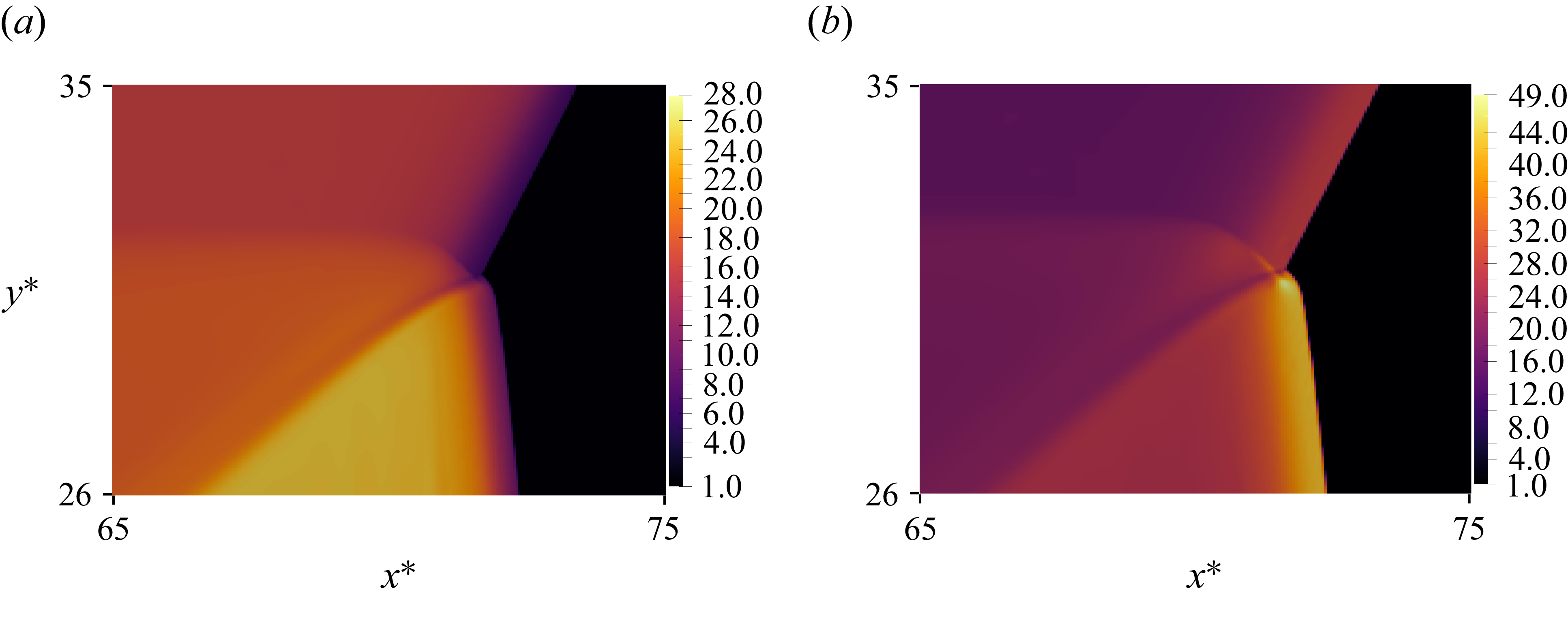
Simulation results cropped to areas of interest for: (a) 10-moment: density; (b) Euler: density; (c) 10-moment: temperature; (d) 10-moment:
 $\tilde {T}_{xx}$
.

Resolved triple-point structure as predicted by the diatomic 10-moment model. (a) Pressure, (b) sketch, (c) velocity magnitude, (d) density.

Figure 9. Long description
Panel A: A contour plot shows the pressure distribution in a one-dimensional shock wave. The x-axis ranges from 65 to 75, and the y-axis ranges from 26 to 35. The color scale on the right indicates pressure values from 1.0 to 210.0. Arrows within the plot indicate the direction of flow. Panel B: A sketch illustrates the shock wave structure, including the connecting shock, reflected shock, incident shock, Mach shock, shear layer, and hot spot. The x-axis ranges from 65 to 75, and the y-axis ranges from 26 to 35. Panel C: A contour plot displays the velocity magnitude in the shock wave. The x-axis ranges from 65 to 75, and the y-axis ranges from 26 to 35. The color scale on the right indicates velocity magnitude values from 1.2 to 13.0. Panel D: A contour plot shows the density distribution in the shock wave. The x-axis ranges from 65 to 75, and the y-axis ranges from 26 to 35. The color scale on the right indicates density values from 1.0 to 12.0.
Figure 8, shows in more details the density, temperature and translational-temperature distributions around the Mach reflection. In this work, the translational temperature,
 $\tilde {T}_{xx}$
, is defined as the temperature along the principal stress axis
 \begin{align} \tilde {T}_{xx} = \frac {\tilde {P}_{xx}}{\rho } \quad \text{with} \quad \tilde {P}_{xx} = \frac {P_{xx} + P_{yy}}{2} + \sqrt {\left ( \frac {P_{xx} - P_{yy}}{2} \right )^2 + P_{xy}^2} \ . \end{align}
For both the viscous (figure 8 a) and inviscid (figure 8 b) solutions, the forward jet can be clearly identified. The Euler solution predicts a slightly larger vortex located closer to the Mach stem pushing the shock wave forward. The Kelvin–Helmholtz roll-ups visible along the slip line of the Euler solution (figure 8 b) are absent from the 10-moment solution computed on an identical mesh, indicating that their absence reflects physical momentum diffusion. This is confirmed quantitatively by the Reynolds number. Using the definition of Rikanati et al. (Reference Rikanati, Sadot, Ben-Dor, Shvarts, Kuribayashi and Takayama2006) and Lau-Chapdelaine & Radulescu (Reference Lau-Chapdelaine and Radulescu2016)
 \begin{align} {Re} = \frac {U_{\textit{shear}}\,h_{M}}{\nu _{{c.s.}}} = \frac {\rho _{{c.s.}}\,U_{\textit{shear}}\,h_{M}}{\mu }, \end{align}
with the tangential velocity jump
 $U_{\textit{shear}}\approx 3$
, Mach-stem height
 $h_{M}\approx 41$
, mean free path (
 $\lambda _{\textit{ref}}$
),
 $\rho _{{c.s.}}\approx 7.2$
and constant viscosity
 $\mu ^{*}=0.83$
, we obtain
 ${Re}\approx 1\times 10^{3}$
at
 $t^{*}=17$
. This lies more than an order of magnitude below the critical value
 ${Re} = 2\times 10^{4}$
identified by Rikanati et al. (Reference Rikanati, Sadot, Ben-Dor, Shvarts, Kuribayashi and Takayama2006) for transition to turbulent growth in shock-reflection shear layer. The temperature profile (figure 8
c) shows that the hottest region is found behind the Mach stem, more precisely along the slip line. At this scale, the highest translational temperature
 $\tilde {T}_{xx}$
is recorded within the post-reflection Mach shock structure (figure 8
d).
In order to further investigate the triple-point configuration, high-resolution calculations of its structure are presented in figures 9 and 10. The pressure distribution (figure 9
a) shows that all three shocks have a distinct structure. The incident shock is observed to transition smoothly into the reflected shock. Furthermore, the confluence of the Mach shock and the incident shock creates a discontinuity within the triple point, which we call the ‘connecting shock’. The span of the connecting shock is dictated by the width of the incident shock, as depicted in figure 9(b). Ultimately, it is the interaction between the foot of the connecting shock and the lead fronts of the Mach shock and incident shock that is responsible for creating this particular configuration. Streamlines, computed in the triple-point reference frame, are also displayed in figure 9(a). The streamlines indicate that the flow is redirected within the incident shock structure to cross the connecting shock normally. The density profile extracted along a line normal to the connecting shock is shown in figure 11. The sampling line, identified by the white arrow in figure 11(a), spans approximately
 $l^* = 2.8$
mean free paths. Beginning in the unshocked gas, the profile first intersects the incident shock at
 $l^*\approx 0.4$
, producing a sharp density increase. The density then rises more gradually through the compressed region behind the incident shock before undergoing a second pronounced jump at
 $l^*\approx 1.0$
, where the line crosses the connecting shock. Beyond this point, the density continues to increase until the line approaches the shear-layer region. The velocity magnitude,
 $u_{{TP}}^*$
(figure 9
c) shows a thickened shear layer where its width corresponds to the connecting shock length. A smaller density jump is also observed at the intersection between the foot of the connecting shock and the Mach stem forming the leading edge of the slip line (figure 9
d).
Resolved triple-point structure as predicted by the diatomic 10-moment model. (a) Temperature, (b) translational temperature.

Density profile following a path crossing the connecting shock. (a) Density, (b) density profile.

The temperature field indicates that the hottest part of the configuration is located behind the Mach shock and along the slip line. However, a particularly important feature of the resolved triple-point structure is the formation of a localised translational-temperature hot spot. As shown in figure 10(b), the peak value of
 $\widetilde{T_{xx}}$
in this region is approximately
 $20\,\%$
higher than the temperature recorded behind the Mach stem. This local enhancement is produced by the extension of the connecting shock into the Mach shock, which creates a strongly non-equilibrium interaction region within the triple point. The results therefore confirm that triple points cannot, at this scale, be regarded as simple discontinuous intersections of three shocks and a slip line. Rather, they possess a complex internal structure in which shock overlap, flow redirection and temperature anisotropy combine to generate localised thermodynamic states that differ substantially from those predicted by local equilibrium.
These findings may have important implications for gaseous detonations, where triple points are fundamental elements of the cellular front. In such flows, triple points repeatedly interact with transverse waves, shear layers and shock-processed pockets of gas. In this setting, the internal non-equilibrium structure of the triple point could affect the induction process and modify local hot-spot formation, especially in mixtures with fast chemistry.
Although the diatomic 10-moment model accurately captures anisotropic stresses and translational–rotational non-equilibrium, as demonstrated by the MD calculations, it does not admit an independent heat-flux description. Because the closure is based on a Gaussian velocity distribution, second-order moments may depart from equilibrium, but third-order moments remain constrained. The model is therefore expected to be less accurate in regions where heat flux plays an important role. Higher-order moment closures could, in principle, improve the description by incorporating additional moments, but such models often face practical difficulties, including restricted realisability and possible loss of hyperbolicity in strong shock calculations. For this reason, further confirmation using higher-order moment models or high-fidelity MD simulations would be valuable.
7. Conclusion
In this work, the non-equilibrium structure of triple points was investigated using a diatomic extension of the 10-moment model. The model was first assessed using a simpler one-dimensional shock problem by comparing resolved shock structures with NSF and MD calculations. These comparisons showed that the 10-moment model captures the translational–rotational relaxation process with good accuracy and provides a more accurate description of the downstream non-equilibrium shock structure than the classical Navier–Stokes description.
The reflection of a triple-shock configuration from a plane of symmetry was then studied numerically in two dimensions. This configuration isolates the evolution of a Mach reflection and the newly formed triple point. At the large scale, the 10-moment and Euler solutions were found to be in good agreement, indicating that the principal hydrodynamic features of the reflection are robust. At the small scale, however, triple points cannot be regarded as simple gas-dynamic discontinuities. The calculations show that all three shocks possess a finite structure, where the incident shock transitions smoothly into the reflected shock, and the confluence of the Mach shock and incident shock gives rise to an internal discontinuity, referred to here as the connecting shock.
A principal result of the present work is that the internal structure of the triple point contains a strongly non-equilibrium interaction region. In particular, the extension of the connecting shock into the Mach shock generates a localised translational-temperature hot spot whose peak value is approximately
 $20\,\%$
higher than the temperature recorded within the Mach stem. This demonstrates that the triple point possesses an intrinsic internal structure with localised temperature anisotropy.
These findings are potentially important for gaseous detonations, in which triple points are fundamental elements of its cellular structure. Localised translational-temperature enhancement within the triple-point structure may modify the induction process and promote hot-spot formation in mixtures with sufficiently fast chemistry. The present results therefore suggest that the small-scale non-equilibrium structure of triple points may influence the larger-scale dynamics of cellular detonations.
Funding
This work was supported by AFOSR grant FA9550-23-1-0214, with Dr C. Li as program manager and by NSERC Discovery Grant RGPIN-2025-04197 ‘Towards a predictive model of the cellular detonation structure in gases’.
Declaration of interests
The authors declare that they have no known competing interests.

 t∗=10


 t∗=17

 t∗=17

 T~xx



 Open access

