1. Introduction

The Antarctic pack ice plays an important role in global climate and climate change (e.g. Reference BuddBudd, 1991; Reference HannaHanna, 1996), particularly due to the large seasonal variability in ice extent and thickness, and the presence of leads and polynyas. The heat provided to the underside of the ice from the ocean, the so-called oceanic heat flux (OHF), is very important to ice growth and decay, and a key term in the mass and heat balance of sea ice. However, there are very few direct measurements of the OHF available to date. Reference AllisonAllison (1981) and Reference Allison, Tivendale, Akerman, Tann and WillsAllison and others (1982) reported an annual mean OHF of 10−15 Wm−² under coastal fast ice near Mawson, with a maximum value up to 40 Wm⁻² in early winter. Reference Heil, Allison and LytleHeil and others (1996), using a thermodynamic model, derived an average OHF of 7.9 Wm⁻², with an annual mean ranging from 5 to 12 Wm"² for fast ice over the period 1958−86 in the vicinity of Mawson, on the coast of East Antarctica. Reference Gordon and HuberGordon and Huber (1990) estimated similar values of 16 Wm⁻² for the annual average and 41 Wm"² for the winter period along the Greenwich meridian at 60−70° S. Reference MartinsonMartinson (1990) obtained results in agreement with those estimated by Reference Gordon and HuberGordon and Huber (1990) from an analytic model analysis. Reference Lytle, Massom, Bindoff, Worby and AllisonLytle and others (2000) derived an average OHF of 15 Wm⁻² in the East Antarctic region around 140° E, 64° S during August 1995. A high value of winter OHF has also been reported by Reference McPheeMcPhee and others (1996, Reference McPhee, Ackley, Kottmeier and Morison1999) in the central Weddell Sea. In the western Weddell Sea the estimated winter OHF is relatively small, only about 7 Wm⁻² (Reference Lytle and AckleyLytle and Ackley 1996) from late February to early June. All of these measurements illustrate the uncertainty of the OHF and its high degree of variability in space and time.

The OHF has been prescribed as a constant in many sea-ice models, due to the lack of observational data (Reference Parkinson and WashingtonParkinson and Washington, 1979; Reference Hibler and AckleyHibler and Ackley, 1983), although in some sea-ice models it is parameterized to be dependent on water temperature (e.g. Reference Ebert and CurryEbert and Curry 1993). Values used range from 2 to 25 Wm⁻². Reference Parkinson and WashingtonParkinson and Washington (1979) used a high OHF value of 25 Wm"² to obtain a realistic seasonal cycle of sea-ice distribution in the Southern Hemisphere. However, Reference Hibler and AckleyHibler and Ackley (1983) used only 2 Wm⁻² to obtain a realistic seasonal cycle of the Weddell Sea ice when they used daily, rather than monthly, atmospheric forcing. They suggested this was a result of the role of ice dynamics in their model. From simulations of the Southern Ocean ice-ocean system, using a coupled ice-ocean model with atmospheric data forcing from the European Centre for Medium-range Weather Forecasts climatology, Reference HäkkinenHäkkinen (1995) suggested that the averaged OHF in the Weddell Sea is < 20 Wm⁻². Reference Geiger, Hibler and AckleyGeiger and others (1997) also demonstrated that a constant value of 20 Wm⁻² of OHF is too high for the Weddell Sea. They showed that the use of a higher value in the east than in the west, and higher in winter than in summer, based on observations, produced a better simulation of the seasonal cycle of the Weddell Sea ice.

Ideally, the OHF should be able to be calculated as a residual based on the energy and mass conservation over the sea-ice zone and it should be diagnostic in a fully coupled ocean model. However, the existing datasets acquired from observations do not cover adequately the complete seasonal cycle within the Antarctic sea-ice zone. Fully coupled models usually need to include ocean surface heat-flux corrections to avoid climatic drift, and also require long computation time to reach equilibrium climates. In this study we test the sensitivity of the simulated Antarctic sea-ice distribution to OHF in a coupled atmosphere-sea-ice model. The sea-ice model is an extension of the model ofReference Wu, Simmonds and BuddWu and others (1997) and includes an ice-thickness-dependent rafting scheme in the ice dynamics (Reference Worby and WuWorby and Wu, 1998; Reference Wu, Budd, Lytle and MassomWu and others, 1999). The sea-ice distributions modelled for different prescribed OHF values are compared with observations. Passive-microwave remote sensing of sea ice provides data on ice extent, ice concentration and open-water fraction. Ice-thickness data have been obtained from in situ ship-based observations.

2. Model Description

3. Datasets for Validation

The observational data for sea-ice concentration are derived from satellite observations: the Special Sensor Microwave/ Imager (SSM/I) from July 1987 to June 1995. These data provide daily global coverage of the Antarctic sea-ice zone. However, there is still considerable uncertainty in the climatology with regard to the global sea-ice cover because of its large regional and interannual variability, the uncertainties in the radiance to ice-concentration algorithm, and the relatively short period of global data available (Reference Cavalieri, Gloersen, Parkinson, Comiso and ZwallyCavalieri and others, 1997; Reference Comiso, Cavalieri, Parkinson and GloersenComiso and others, 1997).

The sea-ice thickness data used here are primarily from in situ observations from 18 voyages to the East Antarctic pack-ice zone between 1986 and 1995. The observations were made hourly from the ship’s bridge using a technique described by Reference Worby, Massom, Allison, Lytle, Heil and JeffriesWorby and others (1998). For each observation the pack is divided into three thickness categories, and the concentration, mean thickness, floe size, topography and snow cover are estimated for each category. The dataset covers the months March-April and August-December. The monthly ice- and snow-thickness distributions from these data are presented in Reference Worby, Massom, Allison, Lytle, Heil and JeffriesWorby and others (1998).

4. Simulation Results

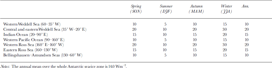
The coupled atmosphere-sea-ice model described in section 2 was used to simulate the seasonal cycle of the global sea-ice distribution, but it is the Antarctic simulation which forms the primary focus of this paper. To study the sensitivity of the Antarctic sea-ice distribution to OHF in the coupled atmosphere-sea-ice system, we run the model using prescribed OHF of 0, 5, 10, 15, 20 and 25 Wm⁻² (hereafter OHF0,…,OHF25). The OHF is fixed at these values through the whole year within the ice-covered area (i.e. whenever sea ice exists the OHF is applied). We have also run the coupled model with prescribed seasonally and spatially variable OHF based on limited available observations as shown in Table 1. In this run the OHF is varied to be higher in winter and lower in summer, and is set higher in the central and eastern Weddell Sea (35°W-20°E), than over the other regions, with the minimum in the western Weddell Sea (60−35° W). We have also used higher OHF in the western Ross Sea (160° E-160° W). This is based on the residual ice in the constant-flux cases. The variable heat-flux experiment is referred to as VAR. To gain an appreciation of the importance of the role played by ice advection in the sea-ice model, we have also performed an experiment using the same OHF as in VAR but without ice advection (i.e. using thermodynamics only). This experiment is referred to as VART. All experiments were run for 6 years with the same initial conditions from an early quasi-equilibrium simulation. The results presented here are from the 4 year average from years 3−6 of the simulations (the first 2 years’ results are treated as adjustment).

Table 1.

The prescribed seasonally variable ohf used in the var and VART experiments for seven sectors of antarctic ice cover

The sea-ice extent, which is defined as the area with sea ice present (including open water) for which each gridcell has at least 15% sea-ice concentration, is very sensitive to the OHFin late spring and summer, but less so for the rest of the season. The simulations for VAR and OHF15 compare well with observations, but for OHF0−OHF10 and VART there is too much sea ice in summer, and for OHF20 and OHF25 there is too little sea ice simulated (see Figs 1 and 2). The simulated sea-ice concentration (not shown) is reasonable compared to SSM/I data, but values tend to be 5−15% higher. The SSM/I gives a mean sea-ice concentration of 46% for December-February (DJF) and 70% for June-August (JJA). The corresponding simulation is 44−59% for DJF and 81−82% for JJA, except forVARTwhich is 80% for DJF and 85% for JJA. However, one should bear in mind that there is still some concern that the satellite-estimated sea-ice concentration is too low during winter in regions of thin ice and brash (e.g. Reference Comiso, Cavalieri, Parkinson and GloersenComiso and others, 1997; Reference Worby and WuWorby and Wu, 1998).

Fig. 1.

Simulated sea-ice thickness (m) for december-february (DJF) average for (a) ohfo, (b) OHF5, (c) OHF10 and ( d) OHF15 the dashed line is the observed (SSM/11987−95 average) sea-ice edge (defined as 15% sea-ice concentration).

Fig. 2.

Simulated sea-ice thickness (m) for DJF average for (a) OHF20, (b) OHF25, (c) var and (d) vart. the dashed line is the observed (SSM/11987−95 average) sea-ice edge (defined as 15% sea-ice concentration).

The Antarctic sea-ice thickness for the different model simulations for DJF average is shown in Figures 1 and 2. The corresponding simulations for JJA are given in Figures 3 and 4. The observed sea-ice edge (defined as 15% sea-ice concentration), from SSM/I data (1987−95 average), is the dashed line in the figures. It can be seen that the OHF has a large impact on the simulated Antarctic sea-ice thickness, and that the sea ice is much thicker in VART (thermodynamics only) than in VAR. More extensive sea ice than observations is simulated for OHF0, OHF5 and VART, and less extensive sea ice for OHF20 and OHF25, in almost every sector of the Southern Ocean in summer. The simulation is reasonable for OHF15 and VAR in summer, except that the sea ice simulated in most of the East Antarctic (45−120° E) is too extensive. This suggests that ice advection plays an important role in ice decay in summer. The sea-ice extent in summer is also sensitive to OHF; an annual mean value of about 15 Wm⁻² for OHF produces a reasonable sea-ice extent. Unlike the summer sea-ice extent the simulated sea-ice edge in winter is reasonable for all experiments including VART, which implies that the advance of Antarctic sea ice is primarily thermodynamic.

Fig. 3.

Simulated sea-ice thickness (rn) for june-august (JJA) average for (a) ohfo, (b) OHF5, (c) OHF10 and (d) OHF15. the dashed line is the observed (SSM/11987−95 average) sea-ice edge (defined as 15% sea-ice concentration).

Fig. 4.

Simulated sea-ice thickness (m) for JJA average for (a) OHF20, (b) OHF25, (c) VAR and (d) VART. The dashed line is the observed (SSM/11987−95 average) sea-ice edge (defined as 15% sea-ice concentration).

Observations show that most Antarctic first-year winter sea ice is 0.4−1.0 m thick (e.g. Reference Wadhams, Lange and AckleyWadhams and others, 1987; Reference Wadhams, Johannessen, Muench and OverlandWadhams, 1994; Reference Worby, Jeffries, Weeks, Morris and JañaWorby and others, 1996, Reference Worby, Massom, Allison, Lytle, Heil and Jeffries1998). This means that the simulated sea ice in VART is too thick; this may also be true for OHF0 and OHF5. For OHF20 and OHF25 the simulated sea ice is clearly too thin. The simulations for OHF10, OHF15 and VAR appear reasonable.

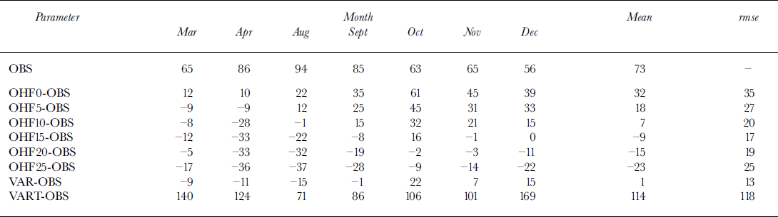
Table 2 shows the observed sea-ice thickness off East Antarctica (60−150° E), and the modelled bias of sea-ice thickness (model less observation). The observed values are derived from observations of the undeformed thickness of floes, plus the contribution to total thickness due to ridging, estimated by Reference Worby, Massom, Allison, Lytle, Heil and JeffriesWorby and others (1998) to be an additional 80% of undeformed floe thickness. The values are also weighted by the open-water fraction to represent the mean over the total ice and leads area. During early autumn (March-April) the mean OHF needs to be about 0−5 Wm⁻² off East Antarctica in order to match the observed sea-ice thickness; during late winter it should be about 10−20 Wm⁻². For December, however, relatively high OHF values (10−15 Wm⁻²) are required within the same region. Although this is less than the value suggested by Reference GordonGordon (1981), there is still a question concerning the physical reason for this. Modelling has shown that the OHF is small in summer because the upper ocean is capped by fresh water from ice melting which effectively stops ocean heat entraining into the surface layer (e.g. Reference Lemke, Owens and HiblerLemke and others, 1990; Reference StosselStossel, 1992). One may argue that for each month the observations do not cover all the area of 60−150° E off East Antarctica as in the model simulation; nevertheless, for the mean ice thickness overall, OHF10, OHF15 and VAR produce reasonable simulations. With statistical analysis, VAR produces the smallest root-mean-square error of all the experiments. For the constant-OHF case, OHF15 produces the best simulation. When only thermodynamics is used, the simulated sea ice is too thick.

Table 2.

The averaged sea-ice thickness (cm) at 60−150° E from in situ observations for march, april and august-december, and the simulated bias (model less observation) and root-mean-square error (rmse) of sea-ice thickness (cm) for different OHF runs (0−25 wm–2, VAR and vart)

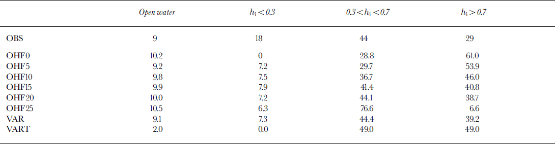
In August and September 1993, an investigation of sea-ice physics and biology was undertaken in the Bellingshausen and Amundsen Seas in the region 66–71 ° S, 77–110° W. Reference Worby, Jeffries, Weeks, Morris and JañaWorby and others (1996) estimated a sea-ice thickness distribution in this region from direct measurements. We have calculated the dependence of the simulated sea-ice thickness distribution on the mean OHF, based on the mean ice thickness at each gridcell, over the same region for August-September, which is shown in Table 3. VAR, OHF15 and OHF20 simulate a reasonable sea-ice distribution compared to the observations. However, the model simulates too little thin ice (ice thickness < 0.3 m) and too much thick ice (ice thickness > 0.7 m) for all experiments, except for OHF25 which shows too little thick ice. This is due to the limitation of the single ice thickness in each gridcell in the model (Reference Worby and WuWorby and Wu, 1998), and also the low spatial resolution of the model. If multiple thicknesses are allowed in a gridcell or the model’s spatial resolution is higher, it is expected that the thin-ice simulation can be improved. Again the worst simulation is VART, which shows too little open water in the ice pack compared to observations, due to the lack of sea-ice advection in this simulation.

Table 3.

Dependence of the simulated sea-ice thickness distribution on mean OHF, over the region 66–71° S, 77–110° win the bellingshausen and amundsen seas, august-september. the thickness distribution is given as the percentage of ice in each thickness category (hi in m)

These simulated results indicate that the OHF varies not only seasonally but also spatially. The annual mean OHF over the Southern Hemisphere is about 10−15 Wm⁻², with higher values in winter, which agrees with observations. The results also suggest that sea-ice dynamics plays an important part in the seasonal distribution of sea ice. The advance of Antarctic sea ice is primarily by thermodynamics, but the rapid decay depends critically on ice advection. This supports the findings of Reference Hibler and AckleyHibler and Ackley (1983), who simulated the seasonal cycle of the Weddell Sea ice.

5. Discussion and Conclusions

This work has focused on the sensitivity of the Antarctic sea-ice distribution to OHF in a coupled atmosphere-sea-ice model, and attempted to define the seasonal cycle of the OHF in the coupled system. Our results indicate that the magnitude of the OHF is critical in determining the sea-ice thickness distribution and the summer sea-ice extent. This is in good agreement with other studies (e.g. Reference Geiger, Hibler and AckleyGeiger and others, 1997). An annual mean OHF of 10−20 Wm⁻² gives a reasonable sea-ice thickness distribution in the Southern Hemisphere, and agrees with the limited observations of OHF available (Reference AllisonAllison, 1981; Reference Gordon and HuberGordon and Huber, 1990; Reference MartinsonMartinson, 1990; Reference McPheeMcPhee and others, 1996, Reference McPhee, Ackley, Kottmeier and Morison1999; Reference Lytle, Massom, Bindoff, Worby and AllisonLytle and others, 2000). Values of 0−5 Wm⁻² for OHF throughout the year will cause the simulated sea ice to be too thick, but when a value of 20−25 Wm⁻² is used throughout the year, the simulated sea ice is too thin to match observations. Our results also indicate that a larger OHF is required in winter, which also agrees with observations. The results from our coupled model differ from those with prescribed monthly-mean atmospheric forcing (Reference Parkinson and WashingtonParkinson and Washington, 1979), but support the findings of Hibler and Ackley (1993) that ice advance is due primarily to thermodynamics but the rapid decay of ice extent depends very much on ice advection. Without advection, sea ice is simulated poorly, being too thick and too compact in all seasons, and too extensive in summer. Observations indicate that the OHF may vary from one region to another. Our results suggest that the OHF in the East Antarctic region differs from that in the Weddell Sea: while a mean value of 15 Wm⁻² is reasonable for East Antarctica, it might be too high for the western Weddell Sea. To test if a seasonally and spatially variable OHF would improve the simulated sea-ice distribution, we have also run the coupled model with prescribed OHF, based on the limited observations available (VAR). We found that a variable OHF simulates the sea-ice distribution better than a constant OHF. This supports the earlier work by Reference Geiger, Hibler and AckleyGeiger and others (1997) who studied the sensitivity of Weddell Sea ice to atmospheric and oceanic forcing.

The OHF has a large impact on the simulated Antarctic sea-ice thickness, which decreases with the increase in OHF. This implies that OHF is of great importance for simulating the sea-ice distribution. Appropriate values of the OHF are as important as ice dynamics for the sea-ice model. For fully coupled climate models, which include the ocean, the OHF is prognostic. There is a need for more accurate values of the OHF from observation to validate the parameterization of the OHF in the models, and to validate the simulated sea-ice distribution under the present climate conditions without the use of imposed heat-flux adjustments.

We have demonstrated the importance of the OHF and also sea-ice advection in the simulated Antarctic sea-ice distribution. However, the OHF is not the only unknown, as there are still some shortcomings in the present model simulations, related to the atmospheric and oceanic forcing. Firstly, there is a lack of explicit ocean-current forcing in the model simulation, which may cause a less realistic sea-ice simulation in some major gyres including the Weddell Gyre. Secondly, there might be some deficiencies in the simulated wind field from the atmospheric GCM (Reference Wu, Simmonds and BuddWu and others, 1997) relative to the synchronous time observations. The simulated sea ice may be constrained by biases of the atmospheric wind and other fields. Thirdly, the 2% free drift might be too low at some locations, and this may reduce the drift rates of the modelled ice to values which are too low compared to observations. Finally, the single ice thickness used in the model allows only a crude estimation of the real thickness distribution. Nevertheless we have successfully simulated the large-scale seasonal sea-ice distribution of the Antarctic sea ice when a value of OHF close to observed values is prescribed in the model which includes sea-ice advection. In the future we propose to use a sea-ice model which includes more complex physics of sea-ice dynamics (e.g. Reference HiblerHibler, 1979) and a multi-level ice-thickness distribution.