

1. Introduction
Sweden's monetary policy during the 1930s is one of the most fascinating episodes in Europe's economic history of the twentieth century. In late September 1931, when Sweden suspended the gold standard, the finance minister made the public statement that from now on, monetary policy would be aimed at stabilising the internal price level. Judging from the record, the goal was achieved rather successfully. It is also impressive to see how intensely contemporaries were debating monetary policy during those years. Eminent economists such as Gustav Cassel, Eli Heckscher and Bertil Ohlin were participating in this public discussion.
Because of the remarkable statement by the finance minister and because Sweden recovered more rapidly from the depression than most other European countries, its monetary policy has repeatedly been invoked as a new model, most enthusiastically by Irving Fisher (Reference Fisher1935). In recent times, it has also been cited as a sort of precursor of today's inflation targeting (Svensson Reference Svensson1995; Bernanke et al. Reference Bernanke, Laubach, Mishkin and Posen1999). In this article, we examine the question of whether or not the Swedish central bank (Riksbank) was in fact targeting the price level.
In spite of the admiration for Sweden's record during the 1930s, this question has only rarely been studied systematically. Besides contemporary scholars, only Lars Jonung and his collaborators have seriously approached the topic (Jonung Reference Jonung1979a, Reference Jonung1979b; Berg and Jonung Reference Berg and Jonung1999; Fregert and Jonung Reference Fregert, Jonung, Burdekin and Siklos2004).Footnote 1 This new research has led to a revision of Fisher's enthusiastic view. Jonung and Fregert (2004) acknowledge that the Riksbank became ‘the first and so far the only central bank to have adopted price stabilisation or price-level targeting as the guideline for its activities’. But they also point out that the Riksbank ‘appears to have given priority to exchange-rate stabilisation over price stabilisation’.
Based on new econometric and narrative evidence, we propose a different revision of Fisher's view. While confirming the Riksbank's strong bias towards exchange-rate stabilisation, we argue that this finding can hardly be reconciled with the claim that the Riksbank adopted price-level targeting. Our results suggest that the Riksbank did not reorient its policy after 1931, but continued to follow the monetary policy of the Bank of England and was targeting the sterling rate of the krona. Although being a major innovation in the history of Swedish economic thought, price-level targeting had no practical importance for the decisions of the Riksbank in the 1930s. There was a large gap between official declarations and actual policies pursued by the central bank – the same gap that has recently been observed with respect to the exchange-rate policies of emerging markets (Calvo and Reinhart Reference Calvo and Reinhart2002; Reinhart and Rogoff Reference Reinhart and Rogoff2004; Levy-Yeyati and Sturzenegger Reference Levy-Yeyati and Sturzenegger2005). Swedish monetary policy was essentially made in London, before as well as after the devaluation of the krona in September 1931.
This finding has implications for the prevailing view of the interwar years as a decade of great policy innovations. Even in Sweden, where eminent economists came up with original and far-sighted ideas, policy makers were reluctant to abandon the notion that there was no alternative to a fixed-exchange-rate regime. The paper standard was regarded as a temporary measure, but not as an opportunity to pursue a more autonomous monetary policy. The most important argument in favour of a conservative approach was that the exporting sectors would be negatively affected by a floating exchange rate. Only in the last quarter of the twentieth century did this conviction give way to a more positive view towards exchange-rate flexibility.
The remainder of the article is organised as follows. Section 2 gives a survey of the exchange-rate regimes adopted by Sweden and its Scandinavian neighbours. Section 3 summarises the official declarations which are the basis for the claim that the Riksbank in fact adopted price-level targeting. Sections 4 and 5 present our new econometric and narrative evidence. The article ends with a short conclusion.
2. Scandinavian monetary policy during the interwar years
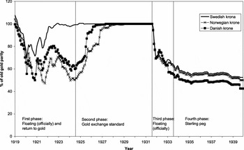
To capture the basic features of Swedish monetary policy during the interwar years, we first consider the Scandinavian context.Footnote 2 As for many other European countries, the monetary history of Denmark, Norway and Sweden during the interwar period can be divided into four phases (Figure 1).Footnote 3 In the first phase, beginning in 1919 and characterised by floating exchange rates, Denmark, Norway and Sweden were trying to bring their currencies back to the gold standard at the prewar parity. The three countries varied considerably with respect to the point in time at which they achieved this goal. Sweden was first: the krona was tied back to gold in April 1924, one year before Great Britain took this step. Denmark and Norway experienced more problems, mainly because of a particularly severe banking crisis in the early 1920s. The de jure restoration of the gold standard occurred in Denmark in January 1927 and in Norway in May 1928.
Scandinavian exchange rates (percentage of prewar gold parity, monthly data)

The second period lasted from the restoration of the gold standard until its fall in September 1931. All three Scandinavian countries followed the devaluation of the pound within days. For Denmark, the main reason was the high share of exports to the British market. No less than 60 per cent of Danish agricultural products were shipped to the British ports. Norway's decision to suspend the gold standard was motivated by the importance of sterling for the shipping business. For the Swedish Riksbank, the main problem was of a financial nature. In the course of 1930, some Swedish commercial banks had accumulated a substantial foreign short-term deficit in order to provide the financier Ivar Kreuger with liquidity. When in July 1931, the German banking crisis broke out, triggering a general rush for liquidity, the banks covered their foreign short-term deficit by buying exchange reserves from the central bank. Consequently, when the British pound was devalued and another attack on the krona was launched, the Riksbank had too few reserves to defend the old parity.
In the third phase, lasting from the autumn of 1931 to the summer of 1933, the currencies were officially floating. The Scandinavian countries chose different paths. Denmark engineered a competitive devaluation in January 1933 after New Zealand, its main competitor in the British market for agricultural products, had done so. When suspending the gold standard, the Norwegian and Swedish authorities declared that they would aim at stabilising the purchasing power of the currency. In Sweden, the Riksbank constructed a new consumer price index, while the government, the Riksdag, and several economists extensively discussed monetary policy matters in public. In Norway, by contrast, the official statement of September 1931 was not followed by a new framework.
The fourth phase began with the decision of all three Scandinavian countries to tie their currencies to sterling. The peg lasted from July 1933 to the outbreak of World War II: the Danish krone was 23 per cent above the old sterling parity, the Norwegian krone 10 per cent, and the Swedish krona 7 per cent. The peg was questioned a few times. In 1935, Danish farmers were demanding a second competitive devaluation; and in late 1936, some Swedish economists pleaded for a revaluation of the currency after a considerable increase in British wholesale prices. In the end, however, the pegs were maintained at the same parity.
3. The official declarations
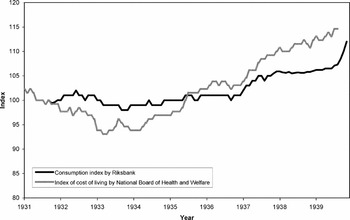
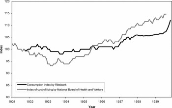
The claim that the Riksbank adopted price-level targeting after the suspension of the gold standard in September 1931 rests on two pillars. The first one is the relative price stability Sweden enjoyed after abandoning the gold standard. Whereas the US and the gold bloc countries continued to experience deflation well into the 1930s, Sweden's domestic price level remained almost perfectly stable after September 1931. Only in two periods were there notable deviations from price stability as measured by the index of consumption constructed by the Riksbank: in early 1933 and in the first two quarters of 1937 (Figure 2).
Index of cost of living by the Riksbank and National Board of Health and Welfare (monthly data)
The second pillar consists of a series of official declarations and reports. It all started on Sunday evening, 27 September 1931, when finance minister Felix Hamrin of the ruling center-right coalition declared that from now on ‘monetary policy should be aimed at stabilising the internal purchasing power of the krona by all means possible’.Footnote 4 The statement, based on ideas of Knut Wicksell and partly drafted by Swedish economists, was supposed to reassure the public that the authorities would prevent inflation after the suspension of the gold standard. Hamrin also declared that Sweden wanted to return to the gold standard as soon as possible. The departure from gold was seen as a temporary measure.
Hamrin's short statement soon became the base for an intensive debate among politicians, central bankers and economists. The Riksbank responded to the new situation by sending a detailed questionnaire to three Swedish economists, Gustav Cassel, David Davidson and Eli Heckscher.Footnote 5 In their answers, returned at the end of October, they agreed on a number of issues. In particular, they all recommended postponing the restoration of the gold standard as long as international financial markets were in turmoil, and favoured stabilising prices at the current level, stressing that the exchange rate should not be fixed, but be used to achieve this goal.Footnote 6 Also in October, the Riksbank constructed a new consumer price index on a weekly basis in order to have a more accurate picture of the dynamics of price movements. Finally, on 11 February 1932, the Riksbank explained its interpretation of the new monetary programme in a letter requesting the government to renew the provisional suspension of the gold standard.Footnote 7 The intention, the Board wrote, was to stabilise the average level of domestic consumer prices, but it would allow a moderate increase in the price index within a certain range insofar as it was caused by external movements such as rising import and export prices or appreciating foreign exchange rates. On the other hand, an increase of the price index caused by domestic inflation would not be tolerated. The Board also emphasised that indicators other than price indices were being taken into consideration, particularly conditions affecting productivity and stocks in various industries.
As the Riksbank was under the direct control of both houses of the Swedish parliament (Riksdag), politicians of all parties began to be involved in the debate.Footnote 8 In May 1932, the Banking Committee drafted a detailed report aimed at developing a more precise monetary programme which became the new basis for all further discussions.Footnote 9 Three points are worth mentioning. First, the Committee rejected the idea of tying the krona to gold or the British pound and argued that the domestic price level and ‘the needs of our own economy’ should be the starting point for monetary policy. Second, it wanted the Riksbank to prevent both inflation and deflation, but also advocated a moderate rise of the price level. And third, the Committee encouraged the Riksbank to keep interest rates as low as possible. In June 1933, the Banking Committee published another report drawing from the recommendations of a committee of experts.Footnote 10 The Banking Committee gave the instruction to engineer a rise in the internal wholesale price level without causing inflation, and provided the Riksbank with more independence, explicitly stating that the choice of instruments was up to the central bank.Footnote 11
Taken together, it is beyond doubt that these official declarations represented a major innovation in Europe's history of monetary policy. For the first time, there was a serious public discussion about how to stabilise the internal price level in the absence of an international monetary system of fixed exchange rates. The crucial question, however, is whether or not this discussion had any practical meaning for the policy of the Riksbank. Berg and Jonung (Reference Berg and Jonung1999) as well as Fregert and Jonung (Reference Fregert, Jonung, Burdekin and Siklos2004) come to the conclusion that the Riksbank in fact adopted price-level targeting and therefore had to accept certain restrictions. The following two sections develop a more sceptical view of Sweden's monetary policy in the 1930s.
4. Narrative evidence and descriptive statistics
A series of statements by the Riksbank governor Ivar Rooth suggest that the Swedish central bank did not implement what was said in public by the Finance Ministry and the Banking Committee of the Riksdag. Of course, besides Rooth there were other personalities trying to determine the course of Sweden's monetary policy. In particular, Ernst Wigforss, Social Democratic finance minister since the autumn of 1932, advocated a stabilisation of the domestic price level.Footnote 12 Likewise, Dag Hammarskjöld, since 1935 adviser to the Riksbank and a close ally of Bertil Ohlin and other economists of the so-called Stockholm School, supported a modern approach (Jonung Reference Jonung1991). But as shown below, the narrative sources clearly suggest that the governor was by far the most influential figure.
We studied the minutes of the Governing Board and the official publications. To have more direct access to the inner thoughts of policy makers, we also looked for sources of private communication. Two discoveries were of particular value: the correspondence of the Bank of England with the Riksbank and other Swedish authorities, and the private correspondence of Ivar Rooth, the governor of the Riksbank.Footnote 13
These latter documents clearly show that the Riksbank never intended to adopt price-level targeting, but was primarily concerned with maintaining a stable exchange rate of the krona vis-à-vis sterling. We cite three letters in order to support our claim. In late September 1933, Rooth wrote to O. M. W. Sprague, Harvard professor of economics and temporary assistant to the United States Secretary of the Treasury.Footnote 14 For obvious reasons – the US had suspended the gold standard in the spring of 1933 –, Sprague was interested in the Swedish experience with managing its currency. Rooth answered that in the months following the fall of the krona, the Riksbank was mainly concerned with emergency measures. It replenished its foreign exchange reserves and was coping with the consequences of the Kreuger crash. But by the end of May 1932, once these problems were solved, ‘we decided to try to keep sterling steady around 19.50 which was the actual level at that time’. Rooth gave four reasons for the sterling peg: to help exports, to stop deflation, to increase liquidity which drove down interest rates, and to encourage Swedish holders of foreign bonds to repatriate their money and to sell their foreign exchange to the Riksbank. Thus, stabilising prices was only one of four major goals. A stable exchange rate was the priority, not price-level targeting. Therefore, Rooth concluded:
My personal opinion is that it is of the utmost importance to the whole economic life of a nation which like Sweden for its standard of living is to such a great extent depending upon foreign trade, to have fairly stable quotations. I think that I dare say that also in order to get a rising price-level, stable foreign exchanges are better than the erratic movements of these rates which the world has suffered from ever since September 1931.
There had only been one episode, Rooth added, in which the Riksbank deviated from this course. At the end of October 1932, when the British pound weakened against the US dollar, ‘we unpegged sterling’, as he put it, and let the krona appreciate considerably. But only six months later, after the Swedish currency depreciated back to the level of 19.50 kronor per pound sterling, the peg was restored.
A second citation is taken from a critical comment Rooth gave on Bertil Ohlin's speech in Zurich in early 1936.Footnote 15 Rooth rejected Ohlin's claim that the Riksbank had sought a stable exchange rate vis-à-vis sterling, because it shared the same monetary policy goals as the Bank of England. The true reason had been, he argued, that Sweden's foreign business was for the most part invoiced in sterling: ‘It was particularly important for a small country like Sweden depending so strongly on its foreign trade to inspire trade and industry with trust in our currency.’ The stable sterling rate, he went on, had also contributed to the transmission of the inflationary tendency of English prices to Sweden. And he concluded that pegging the krona to sterling and lowering interest rates were ‘the only thing we did in order to influence prices’.Footnote 16
A third statement is even more telling. In February 1938, Rooth wrote to Randolph Burgess, vice-president of the Federal Reserve Bank of New York:
Some American professors, e.g. Professor Irving Fisher, believe that it is an achievement by us in the Riksbank that prices have been fairly steady up to the middle of 1936. I have told Professor Fisher before and I am sorry to have to tell you now that what we have done is merely that we have carried out a fairly conservative central banking policy. In fact we have never tried to do anything directly with regard to prices.Footnote 17
Of course, all three of Rooth's statements are ex-post assessments. But there is sufficient evidence suggesting that his memory did not distort the past in a fundamental way. Other archival sources confirm that the Riksbank's main concern was to have a stable sterling parity. It reached this goal by following the policy of the Bank of England, and by first accumulating and then actively managing foreign exchange reserves. Certainly, Rooth was also concerned about prices. But drawing from his experience during the gold standard period, he was convinced that only a stable exchange rate could provide a reliable nominal anchor and thus guarantee price stability in the long run. The domestic purchasing power of the krona, he stated shortly after the suspension of the gold standard, was ‘certainly not a sufficiently firm foothold’.Footnote 18 He appears to have made a correct statement when explaining that the Riksbank had practised a fairly conservative central banking policy.
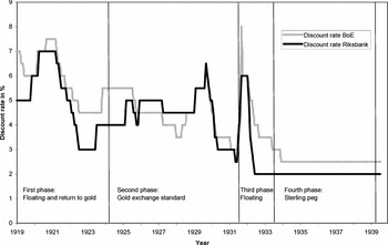
As for setting the discount rate, the minutes of the Board show that the Riksbank wanted to make sure the Swedish rate would never fall below the British one, and it was only ready to lower it when the Bank of England took the same step (Figure 3). The only time the Board acted on its own was in the aftermath of the suspension of the gold standard in September 1931. On 8 and 19 October, it cut the discount rate from 8 to 6 per cent, whereas the Bank of England kept it at 6 per cent. These decisions, however, were not the expression of an independent course, but resulted from the insight that in order to contain inflation after a steep depreciation of the krona it was not necessary to have such a high interest rate.Footnote 19 The Riksbank had decided to increase the discount rate from 6 to a record high of 8 per cent on 27 September, i.e. on the same day finance minister Hamrin announced the suspension of the gold standard and made his famous statement on the future course of Sweden's monetary policy. The exceptionally high interest rate was part of the campaign to reassure the public that the authorities would not allow inflation to emerge and investors to speculate against the krona.Footnote 20
Discount rates of the Bank of England and Riksbank (monthly data)

A clear sign that Rooth consciously avoided stepping out of line with British policy is his opposition to a discount rate cut on 14 January 1932.Footnote 21 One member of the Board proposed it because Swedish business leaders had protested against the restrictive policy for some time, but Rooth prevailed with his cautious approach. Only when the Bank of England lowered its rate from 6 to 5 per cent on 18 February, was he ready to relax monetary conditions, although still reluctantly. On the same day he wrote to London that he was very surprised by the British decision and asked ironically: ‘What has happened? Has any of the Indian maharadjas sent you all their gold, are you preparing a conversion of the Warloan or have you decided to follow the suggestion made in the last copy of The Economist, viz. to “reflate” the prices to the level of 1928?’Footnote 22 Due to his mistrust of expansionary policies, Rooth proposed to follow the Bank of England only halfway to 5.5 per cent and to wait for the consequences.Footnote 23 Two weeks later, with the fear of inflation diminishing, the Riksbank lowered the discount rate by another half per cent in order to bring it down to the British level – the reference to the Bank of England being a crucial argument.Footnote 24 In the following months, the Riksbank continued to follow the British policy, although with some time lag. From March to June, the Bank of England cut the discount rate from 5 to 2 per cent, the Riksbank lowered it to 3.5 per cent in the second and third quarters of 1932 and to 2.5 per cent in the course of the following year. Again, the decisions were inspired by the policy of the Bank of England.Footnote 25
As for the management of the exchange rate, Rooth's memory proved again to be accurate. Only in the immediate aftermath of the suspension of the gold standard did the Riksbank hesitate to seek an exchange rate peg since the situation remained chaotic for some weeks. Rooth considered the stabilisation of the domestic price level only as a temporary policy to prevent inflation and to reassure the public. His next goal was to tie the krona to sterling as soon as the future path of British monetary policy took shape. Accordingly, Siepmann, a close adviser of Governor Montagu Norman, reported to the British Treasury in mid October that, according to Rooth, the Riksbank's attempt ‘to control exchange in such a way as to maintain the stability of internal prices’ was the only alternative ‘in a period of transition’. And he added that before going to a meeting at the Bank for International Settlements (BIS) in Basle, Rooth ‘was frequently asking me over the telephone for indications of our policy’.Footnote 26 One week later, Siepmann summarised another telephone conversation with Rooth: ‘He told me again that Sweden can have no monetary policy except to keep internal prices stable, so far as possible, until our decision is known.’Footnote 27
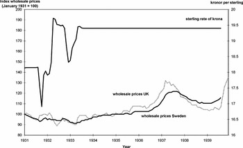
Since the British themselves did not know what kind of monetary policy they should pursue, Rooth did not receive a clear answer. Nevertheless, a few weeks later he became convinced that the moment for a sterling peg had come. His decision was motivated by a rapid fall of the krona against sterling from late October on (Figure 4). According to the minutes of the Board, Rooth had strong reservations against exchange-rate fluctuations and was afraid of speculative attacks against a weakening krona.Footnote 28 A close friend of his, who endorsed the sterling peg, believed that ‘now the British pound plays the role of gold’.Footnote 29 On 18 November, Rooth got the approval of the Board, informed the Bank of England, and turned to the commercial banks for help, since the Riksbank was still suffering from the depletion of its foreign exchange reserves following the defence of the gold standard two months earlier.Footnote 30 He convinced them to ration their credits on a voluntary basis in order to improve the trade balance and to impede speculation against the krona.Footnote 31 Whether or not the agreement with commercial banks stabilised the exchange rate is hard to say, but it almost certainly hampered the recovery of the economy (Lester Reference Lester1939). In any case, Rooth succeeded in implementing his exchange-rate stabilisation scheme, because the krona only temporarily fell below the old sterling parity.
Sterling rate of krona and wholesale prices of Sweden and the UK

Only two months after the declaration by the finance minister and a few weeks after the exchange with the economists about a new monetary policy, the Riksbank violated the new guidelines by seeking a sterling peg at the old parity. The manoeuvre reversed the recovery of wholesale prices. Subsequently, it would have depressed Swedish consumer prices, if the Kreuger crash in March 1932 had not forced the Riksbank to be more expansionary.Footnote 32 Accordingly, the policy was not well received by the press and the political authorities.Footnote 33 In reaction to the widespread criticism, the Riksbank tried to reassure the government of its loyalty by adding a few paragraphs in the upcoming formal request for another renewal of the provisional suspension of the gold standard. As mentioned above, these lines written on 11 February 1932 have been cited as an expression of its commitment to price-level targeting. Yet a closer reading of this key text reveals that the Riksbank, while endorsing the overall goal of price stability, gave only lukewarm support to the new guidelines by pointing out that ‘for the time being each monetary programme can only be valid until further notice’.Footnote 34 Consequently, the Banking Committee of the Riksdag was not entirely satisfied with this explanation and sent a questionnaire while preparing its famous May report cited above.Footnote 35 The committee also tried to ensure a better control of the Riksbank's policy by formulating a more specific monetary programme and openly criticising the deflationary bias of the bank. However, the result of this endeavour was negative. By stating that monetary policy should not only be aimed at stabilising the domestic price level, but also be based based on ‘the needs of the economy’, the monetary programme became fuzzy. The committee also blurred the lines by demanding that monetary policy should not be schematically bound to any special price index. And in any case, further events would show that the views of the deputies were not particularly relevant for the Board of the Riksbank.
The Kreuger crash in mid March 1932 forced the Riksbank to step in as lender of last resort and triggered a selling wave of krona assets. The Riksbank tried to defend the old sterling parity, but due to the lack of foreign exchange reserves, it had to give up its resistance.Footnote 36 The exchange-rate regime remained the same, however: in May, the Riksbank tied the krona back to the British pound at 19.50 kronor per pound sterling – in his letter to Sprague, Rooth referred to this decision as the beginning of the sterling peg which lasted until the end of the 1930s.
In the following months, Swedish wholesale and consumer prices remained almost perfectly stable. The literature has interpreted this restoration of price stability as a success of the Riksdag. The Riksbank, they argue, had to accept certain restrictions imposed by the Banking Committee's May report and thus explicitly adopted price-level targeting.Footnote 37 This view is, however, hard to reconcile with the facts. First, there are no archival sources hinting at a change of mind within the Riksbank. Second, the depreciation of the krona was forced upon policy makers. The Riksbank would have preferred to maintain the old sterling parity regardless of the deflationary effect of such a policy. And third, further events would show that the Riksbank continued to aim for the old parity. The undervaluation of the krona mainly served to replenish foreign exchange reserves in order to have the means to drive the krona towards the former level. The opportunity came in the autumn of 1932, when the British pound weakened considerably. At the beginning of this phase, the Riksbank let the krona depreciate, but after 20 November it stabilised the exchange rate vis-à-vis the US dollar, bringing the krona back to the old sterling parity (Figure 4). When in December the British pound reversed its course and appreciated against the US dollar, the Riksbank maintained this parity, inducing a considerable real appreciation of the krona and a decline of wholesale prices.Footnote 38 The operation failed, however. In early 1933, the krona was not strong enough to follow the British pound in its upward movement and fell back to a lower level, although the Riksbank tried to stem the tide by buying kronor and selling British pounds.
Thus, as in November 1931, the Riksbank openly violated the guidelines set up by the government and the parliament. The first to have noticed it was Lester (Reference Lester1939), who talked to key policy makers at the time. It is difficult to add written evidence to this interpretation because all the minutes of the relevant Board meetings have disappeared. However, we found one clear piece of evidence showing that Rooth wished to bring the krona back to the old sterling parity. In late October 1932, a close friend reminded him of a recent conversation about the future exchange rate of the krona: ‘when I expressed my hope that the krona would appreciate against sterling, you explained that nobody awaited such a movement more eagerly than you’.Footnote 39 In addition, the comparison with the sterling rate of the Norwegian krone is revealing in this respect: whereas the Norwegian krone appreciated only by 2.5 per cent against sterling (from 19.90 in September to 19.41 in December), the Swedish krona climbed by 6 per cent towards the old sterling parity (from 19.50 in September to 18.32 in December). Clearly, the difference was due to the more aggressive exchange-rate management by the Riksbank. It was not a natural result of market forces.
In reaction to this deflationary monetary policy, finance minister Ernst Wigforss of the Social Democrats appointed a committee of experts whose recommendations were adopted by the Banking Committee and the Riksdag. As mentioned, the committee demanded that the Riksbank should allow a moderate rise in the internal wholesale price level, but it was free to implement this strategy how it wished. Besides, it repeated the conclusion of its own report of May 1932 that the krona should not be fixed to gold or to the British pound. Nevertheless, in July 1933 the Riksbank explicitly tied the krona to the British pound at the current rate (19.40 kronor per pound sterling).Footnote 40 According to Rooth's letter to Randolph Burgess, the vice-president of the New York Fed, the Banking Committee's report was irrelevant: ‘In 1933 the banking committee wrote a fairly theoretical programme about the necessity of increasing prices. However, they said that the decisions to be taken in each case had to be made by ourselves and that we had to take the responsibility for the decisions.’Footnote 41 The timing of the decision and the fact that Denmark and Norway established a sterling peg at the same time suggest that two factors were important: the conclusion of a trade agreement of all three Scandinavian countries with the UK in May 1933 and the failure of the London World Economic Conference that became apparent after Roosevelt's bombshell message in early July 1933.
In any case, besides the obvious violation of the Banking Committee's opposition to an exchange-rate peg, the crucial question is whether the krona was pegged to sterling in order to fulfill the monetary programme or in order to stabilise the exchange rate for its own sake. As in the beginning there was no conflict of interest, the question is hard to answer. The price level remained very stable because British wholesale prices and the dollar rate of sterling finally stabilised after an extended period of fluctuations. Yet, when in the second half of 1936 British wholesale and consumer prices increased by roughly 10 per cent, a sterling peg could not be reconciled with price-level targeting anymore. Accordingly, several Swedish economists, among them Gustav Cassel and Eli Heckscher, correctly pointed out that the Riksbank should unpeg the krona from sterling and allow an appreciation in order to keep the domestic price level constant (Figure A2). Investors were also expecting a strengthening of the krona and exchanged foreign exchange for krona – the reserves of the Riksbank almost doubled from the middle of 1936 to late 1937. The Governing Board, however, did not change its policy, although it knew what was at stake. In a letter to Montagu Norman on New Year's Eve, Rooth mentioned that the krona perhaps would be revalued against sterling. Norman remarked in an internal memo:
The Swedes have made a lot of noise about their new monetary policy of basing the level of the krona on a price index and thus maintaining the level of prices. In fact they have up till now had to do nothing but keep pegged on sterling and we have kept their prices steady for them. Rooth is certainly thinking hard about raising the krona rate on sterling, and if sterling prices show a strong rising tendency he will probably do something. His letter is, I think, meant to warn us about this and to express the hope that if and when he moves his rate on sterling we shall pat him on the back and not accuse him of upsetting things and disturbing the currency agreement.Footnote 42
Stockholm's uneasiness also becomes apparent in a note which a senior official of the Foreign Office sent to the Treasury and ultimately to the Bank of England:
At the Swedish Legation last night Mr Sandler [Swedish Minister of Foreign Affairs] took me aside and said that he wanted to ask my views about the Swedish exchange . . . I said that was a matter on which I could offer no opinion . . . there would be no sort of objection from our side if the Swedish Government thought it right to go back to their old parity . . . The question was essentially one which the Swedish Government had to settle by reference to its own internal situation rather than by reference to what was being done in any other country.Footnote 43
By the end of April 1937, when Swedish consumer prices had risen by 4 per cent over the preceding two quarters and did not stop increasing, the Riksbank decided to maintain a stable sterling rate, thus once more violating the principles of price-level targeting.Footnote 44 The arguments put forward by Rooth reveal how strongly he believed in the virtue of having a stable exchange rate. First, he warned of the negative psychological effects of changing the parity. Second, he pointed out that a revaluation of the krona would only temporarily stop the rise of domestic prices. World prices would continue to increase and to drive Swedish prices upward, no matter what the Riksbank was doing. The option of letting the krona float in order to uncouple the Swedish economy from world inflation was not even taken into consideration. In Rooth's view, exchange rate stability was ‘the most important condition for international trade’, whereas flexible exchange rates would only lead to protectionism and hamper trade. Third, a revaluation of the krona would reduce the profitability of the exporting sectors, even more so as Finland and Norway, both direct competitors, were not considering such a step. And finally, he expressed his hope, without giving any evidence, that the rise of British prices would soon stop. Clearly, these arguments were not compatible with a modern monetary policy.
In sum, narrative evidence shows that in four instances the Riksbank consciously acted against the principles of price-level targeting. First, in November 1931, it prevented the krona from falling below the old sterling parity, thus reversing the recovery of Swedish wholesale prices. If the Kreuger crash in March 1932 had not made the exchange rate depreciate by 7 per cent, Sweden would have experienced a marked deflation in 1932. Second, in the last quarter of 1932 the Riksbank made the krona climb to the old sterling parity, thus inducing a steep real appreciation and depressing wholesale and consumer prices. Again, the outcome would have been even worse, if further events had not driven the sterling rate of the krona back to the level where it had been before the adventurous manoeuvre. Third, the Riksbank explicitly pegged the krona in July 1933, although the Banking Committee of the Riksdag had clearly excluded such a policy. And finally, in early 1937 the Riksbank refused to unpeg the krona after British wholesale prices dramatically rose. Instead, by doing nothing it imported inflation and let the domestic price level increase by 5 per cent within two quarters. On the basis of this evidence, it seems hard to maintain the claim that the Riksbank truly adopted price-level targeting. The primary goal was rather to advance the recovery of the exporting sectors by stabilising the exchange rate, first at the old parity, then at an undervalued level.
5. Econometric evidence
To test the qualitative evidence from the previous section, we ran a Bayesian VAR covering the period from 1920 to 1939. In contrast to the traditional structural VAR, the Bayesian approach allows for time-varying parameter matrices and heteroscedasticity, thus enabling us to analyse monetary policy across regime changes not only in terms of changes in the transmission mechanism, but also in terms of a change in the nature of the structural shocks. In particular, we can observe whether or not the end of the gold standard in 1931 represented such a change. The set-up of the model is explained in the Appendix.
The crucial question is whether the Riksbank was trying to stabilise the price level after 1931, as official declarations suggest, or whether it continued to target the sterling rate as under the gold standard regime lasting from 1924 to 1931. We are aware of the fact that these two strategies need not be mutually exclusive. It is possible that the central bank was stabilising the domestic price level by maintaining a sterling peg. The evidence assembled in the last section suggests, however, that the Riksbank was primarily targeting the exchange rate and not the domestic price level. In some periods, the stable sterling rate also delivered price stability, but when in 1936–7 a conflict of interest emerged, the Riksbank was ready to accept an increase in domestic prices, violating the principles of price-level targeting.
The selection of the variables was straightforward. The Riksbank's monetary policy was measured by the discount rate and alternatively the monetary base. We considered both series because the Riksbank did not change its discount rate after 1933 (Figure 3), but the choice of the monetary variable does not change the basic results. To account for the changing relationship between exchange rate and price stability, we chose the British discount rate, the nominal exchange rate (krona against sterling) and two Swedish price indices (wholesale prices and cost of living) as our main variables influencing the Riksbank's monetary policy. The British discount rate was picked because the narrative evidence shows that the Riksbank stabilised the exchange rate by following the discount rate steps taken by the Bank of England.Footnote 45 Finally, to account for other factors possibly influencing the monetary policy of the Riksbank we included two other variables: the business cycle of the real economy and the movement of gold and foreign exchange reserves. To reflect the business cycle, we used union data on Swedish unemployment in the absence of monthly indices of industrial production covering the whole period. It would be surprising if the Swedish monetary authorities had reacted to the output gap as modern central banks do, but is it essential as a control variable. Under the gold standard regime, central banks are supposed to raise interest rates when reserves are approaching or falling below a certain minimum. In Sweden, the legal limit of the gold cover ratio was 40 per cent during most of the period under study. By including foreign exchange reserves in the cover ratio, we have used a broad definition of this indicator. The focus on the gold cover ratio would be too narrow, because it does not account for the reason why Sweden suspended the gold exchange standard in late September 1931. As mentioned above, this regime shift was not primarily due to close trade relations with Great Britain, but to Sweden's foreign short-term debt. Even prior to the fall of sterling, the Riksbank was running out of foreign exchange reserves while the gold reserves remained relatively stable. Only in the final stage did the Riksbank also begin to use them in order to defend the gold standard. More generally, foreign exchange reserves reflect market forces and economic policies better than gold reserves.
In short, the Bayesian VAR has six variables: the discount rate of the Bank of England (I*), the nominal sterling rate of the krona (E), the Swedish unemployment rate (U), the Swedish price index (WPI or CPI), the gold and foreign exchange cover ratio (GCR) and the monetary policy variable (I or M0). The British discount rate can be considered exogenous as it is evident that the monetary policy of the Bank of England was not influenced by the economic development of a small open economy such as Sweden. Moreover, treating I* as an exogenous variable allows a more parsimonious specification of the VAR. The triangular identification scheme for the structural shocks (see equation (2) in the Appendix) is given by the way monetary policy was conducted at the time. The sterling rate E is strongly influenced by the policy conducted by the Bank of England. Therefore, we have ranked it first whereas the following four variables are only indirectly affected by the British business cycle or by British economic policies. We have chosen the nominal exchange rate in order to test whether the Riksbank was targeting the exchange rate or whether it let the krona float while targeting the domestic price level. The unemployment rate U, as noted, is a proxy for Sweden's real economy. As it depends indirectly on the British interest rate and the exchange rate, it ranks second in our model. The consumer price index CPI is included in third rank to test directly whether or not the Riksbank was targeting the domestic price level after 1931. The gold cover ratio GCR was the most important indicator for monetary policy under the gold exchange standard and is therefore ranked immediately ahead of the monetary base, respectively the Swedish interest rate. The monetary data are taken from the Bank of England and the Riksbank, the consumer prices from the Swedish National Board of Health and Welfare (Socialstyrelsen) and the Economist, the unemployment rate from the Swedish Trade Union Confederation (Landsorganisationen). All data are on a monthly basis.
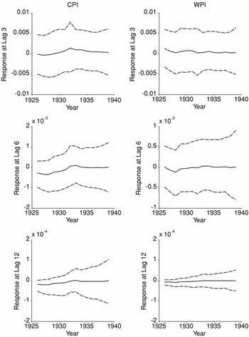
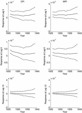
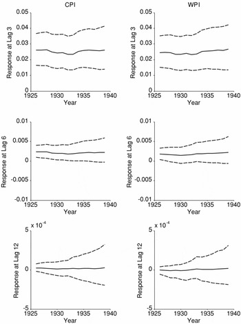
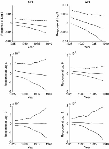
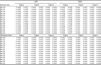
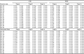
The main results displayed in Figures 5.1 to 5.4 show the posterior distributions of impulse responses (lag 3, lag 6, lag 9 and lag 12). The 95 per cent highest posterior density intervals (lag 3, lag 6 and lag 12) can be found in Tables 1 and 2.Footnote 46
Response of Swedish discount rate to price-level shocks (one standard deviation)

Response of Swedish monetary base to price-level shocks (one standard deviation)

Response of Swedish discount rate to British interest rate shock (one standard deviation)

Response of Swedish monetary base to British interest rate shock (one standard deviation)

Highest posterior density intervals (68 per cent) for the responses to price-level shocks

Note: For an interpretation of highest posterior density intervals, see footnote 46.
Highest posterior density intervals (68 per cent) for the responses to British interest rate shocks
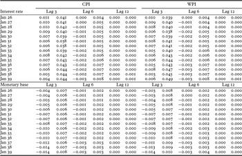
Note: For an interpretation of highest posterior density intervals, see footnote 46.
Did the Riksbank adopt price-level targeting? If this had been the case, we would expect a significant reaction of the Swedish discount rate or the monetary base to a price shock. In both cases, however, the impulse responses reveal quite the opposite. The Swedish monetary policy indicators hardly move, regardless of the choice of price index and the lag. In this respect, the Bayesian VAR provides strong evidence supporting what the statements of the Riksbank governor Rooth suggest. The actual policy did not match the official declarations made by the Finance Ministry and the Banking Committee of the Swedish parliament. Up to lag 6, the Swedish interest rate increases in response to a British interest rate shock. In contrast, when we use the Swedish monetary base we do not see a strong reaction from the Riksbank.
Regardless of the monetary variable we used, the impulse responses strongly suggest that there was no regime change in the early 1930s. This observation amounts to a further argument against the hypothesis that the Riksbank in fact adopted price-level targeting after the suspension of the gold standard in September 1931. Keeping the nominal exchange rate completely stable after 1932, in addition to following the British discount rate without an obvious structural break, requires price levels to adjust – this finding is not in line with stabilising the price level as the target of Swedish monetary policy.
In conclusion, econometric evidence demonstrates that the basic orientation of Sweden's monetary policy remained constant throughout the interwar years and that the Riksbank did not adopt price-level targeting in the 1930s. Its main priority was to maintain a stable exchange rate against sterling by following the discount rate policy of the Bank of England. Thus, the Bayesian VAR strongly supports the main findings drawn from the narrative sources.
6. Conclusion
In the 1930s, Sweden's monetary policy was admired for its success in stabilising the domestic price level after 1931 while most other European countries needed more time to dig themselves out of the deflationary spiral. According to Irving Fisher, the success was due to a regime change in 1931: instead of targeting the exchange rate, the Riksbank from now on aimed its policy at stabilising consumer prices, rather like today's inflation targeters.
Since Jonung (Reference Jonung1979a), this positive view has been revised. In particular, the belief that the Riksbank fully abandoned exchange-rate targeting in favour of price-level targeting has been rejected. Yet, in spite of this strong scepticism towards the actual practice, the new conventional view still claims that the Riksbank truly adopted price-level targeting which imposed certain restrictions on its monetary policy.
In this article, we have tried to show that this view is inconsistent. By employing a Bayesian VAR and analysing new archival sources, we have come to the conclusion that the Riksbank not only gave priority to exchange-rate stabilisation over price-level stabilisation, but also never intended to adopt price-level targeting. As governor Ivar Rooth himself repeatedly pointed out in private letters, his aim was to have stable exchange rates in order to foster trade and to have a strong anchor for monetary policy. Following this conviction stemming from his experience during the gold standard period before and after World War I, he did not hesitate to violate the principles of price-level targeting when he believed that the exchange rate needed to be stabilised.
This finding raises the question as to what extent the 1930s were a defining moment in Europe's monetary history. Sweden has often been cited as an important example of how some policy makers broke with the past. We already know that fiscal policy was much less counter-cyclical and innovative than many observers originally thought.Footnote 47 The results of this article suggest that the same is true for monetary policy. The Riksbank could have pursued a more flexible monetary policy, but it did not even try because policy makers regarded floating exchange rates as harmful to trade and investment.Footnote 48
Acknowledgements
We thank Michael Bordo, Barry Eichengreen, Marc Flandreau, Harold James, Lars Jonung, Peter Kugler, Matthias Morys, Albrecht Ritschl, Scott Urban, Charles Wyplosz, participants at the 7th European Historical Economics Society Conference 2007 in Lund and at the COMMONFACTORS workshop 2007 in Zurich (ESF network GLOBALEURONET) and seminar participants at the University of Basle for helpful comments and suggestions. Support from the Research Priority Programme on Finance and Financial Markets of the University of Zurich is gratefully acknowledged. Finally, we are especially grateful to the Archive personnel at the Bank of England and Mira Barkå, head of the Riksbank Archives, for their support.
Appendix. Time-varying VAR
The vector autoregressive (VAR) model is basend on Primiceri's (Reference Primiceri2005) extension of the approach by Cogley and Sargent (Reference Cogley and Sargent2005). It allows for both time-varying parameters and heteroscedasticity. Consider an n variables VAR of order p with t = 1, . . . T observations:
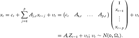
Note that both the parameter matrices Aj,t and the variance-covariance matrix Ωt are time varying. Vectorisation of the last line in equation (1) gives

The error υt has the structure

with
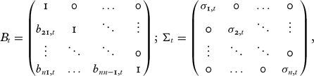
where Σt is the time-varying scaling matrix for the structural shocks ɛt, and Bt is the matrix modelling the contemporaneous interaction between the variables in the system. In the case of Cogley and Sargent (Reference Cogley and Sargent2005), this matrix is constant over time, in the version of Primiceri (Reference Primiceri2005) used here, the parameters are time varying. This has the advantage that the contemporaneous response of the system to structural shocks is time dependent. However, the triangular structure which allows identification does not change over time.
The equations of movement for the elements of the VAR parameter matrices and the components of the variance-covariance matrix are random walks:

The last line ensures that the standard deviations are non-negative. By assumption, the errors are not correlated among each others and follow multivariate normal distributions:
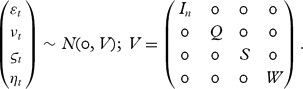
To parameterise as parsimoniously as possible, we fix the order of the VAR to 1, and use UK interest rates as exogenous variables. To arrive at the posterior distribution of the parameters, we have 4 MCMC steps (for details, see Primiceri Reference Primiceri2005):
1. Draw αt conditional on bt, σt, t = 1, . . ., T, and the variance-covariance matrix Q (the variance-covariance matrix for the structural shocks ɛt is fixed to be an identity matrix, see equations 2 and 4). Draws for which the VAR turns out to be unstable are rejected. The prior distribution for αt is independent normal, with expected value and variance-covariance matrix coming from an OLS estimation of a time-constant VAR based on the first 50 observations.
2. Generate bt conditional on αt, σt, t = 1, . . ., T, and the variance-covariance matrix S. The prior distribution of bt is independent normal; the expected value comes from the lower triangular component of an LDL-decomposition of the error variance-covariance matrix of the OLS estimation in step 1, and the variance-covariance matrix is set to the identity matrix.
3. Generate σt conditional on αt, bt, t = 1, . . ., T, and the variance-covariance matrix W. The prior distribution for log σt is also independent normal, with an expected value coming from the diagonal component of an LDL-decomposition of the error variance-covariance matrix of the OLS estimation in step 1, and the variance-covariance matrix is set to the identity matrix.
For steps 1 to 3, the conditional posteriors turn out to be normal. In each case, the underlying model is a state-space model (e.g. Harvey Reference Harvey1992), and the sequence of time varying parameters is generated following the multi-move Gibbs sampling approach proposed by Carter and Kohn (Reference Carter and Kohn1994).
4. In the last step, the variance-covariance matrices Q, S, and W are drawn from an inverted Wishart distribution, conditional on αt, bt, σt, t = 1, . . ., T. The parameters of the inverted Wishart prior for Q come from the OLS estimation in step 1, and for S and W, they are set to I × 1e-2.
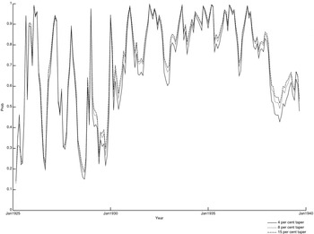
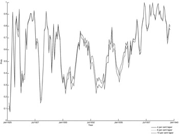
The entire procedure was repeated 60,000 times, and the first 10,000 draws were discarded. After burn-in, we kept every tenth realisation of the chain. To judge convergence of the chain, we calculated the Geweke's χ2 test (e.g. Geweke Reference Geweke2005, pp. 149–50). Since there are too many parameters to look at, convergence is demonstrated for the maximum absolute eigenvalue of the VAR parameter matrix A at each point in time, comparing the mean over a subsample of the first 10 per cent of realisations of the chain with the mean based on the last 50 per cent. The numerical standard errors used to construct this test statistic are based on periodogram estimates at frequency zero with 4 per cent, 8 per cent and 15 per cent autocovariance tapers.Footnote 49 The probabilities that the two means are the same are displayed in Figures A1 (interest rate model) and A2 (money stock model). The figures show that convergence is not a problem here.
Geweke's χ2 test: interest rate model

Geweke's χ2 test: money stock model

It is straightforward to calculate the distribution of the impulse-response matrix at lag j and time t from the distribution of the VAR-parameters and the stochastic volatilities (note that since the lag is set to one, we have just one parameter matrix):