1. Introduction
Among the various robotic systems under consideration for pick-and-place tasks, a 4-DOF robotic arm offers several advantages, particularly in complex industrial scenarios. Unlike higher-DOF systems, a 4-DOF design provides sufficient functionality while reducing costs, complexity, and maintenance requirements.
When it comes to controlling such robotic arms, selecting the right trajectory planning method is essential for ensuring both efficiency and adaptability. Current trajectory planning methods in the 4-DOF robotic arm can be broadly categorized into data-driven method and sample-based optimization.
Data-driven methods [Reference Li, Liu and Dong1, Reference Carron, Arcari, Wermelinger, Hewing, Hutter and Zeilinger2], while more robust, require substantial data and training time. Given that typical pick-and-place tasks are relatively straightforward, such advanced methods may be unnecessary, as simpler approaches can suffice.
Sampling-based optimization methods can be categorized into two main types: those performed in Cartesian space and those performed in joint angle space [Reference Dai, Xiang, Zhang, Jiang, Qu and Zhang3].
Optimization in Cartesian space focuses on planning the trajectory of the robot’s end-effector. While this method is intuitive and allows direct control of the end-effector’s path, it faces challenges with high degrees of freedom. The redundancy in degrees of freedom for positioning a point in 3D space adds complexity, as there is no direct one-to-one correspondence between joint angles and Cartesian coordinates. Additionally, for high DOF robotic arm, it requires complex matrix calculations, making it computationally expensive.
On the other hand, optimization in joint angle space directly plans the motion of each joint, controlling joint angles, velocities, and accelerations. This method avoids the computational complexity of Cartesian space planning and effectively mitigates issues like singularities and redundancy in robotic arms. As a result, joint space planning is widely used for various tasks. It is computationally efficient, supports real-time adjustments, and ensures the continuity of velocity and acceleration. Common methods include polynomial and spline interpolation, with cubic spline [Reference An, Li, Zhang, Man and Zhang4, Reference Xin, Rong, Yang, Xiang and Xiang5] and B-spline [Reference Zhang and Shi6] being particularly useful for maintaining smooth motion.
However, joint space optimization has its limitations. It does not explicitly define the end-effector’s path in Cartesian space. While this reduces computational overhead, it can result in the end-effector’s trajectory being less precise, especially for tasks that require complex movements or obstacle avoidance. Genetic algorithms are often used to optimize joint space planning [Reference Ekrem and Aksoy7, Reference Yue, Henrich, Xu and Tso8], but they struggle with high dimensionality and can easily get stuck in local minima, further complicating the search for optimal solutions in complex environments.
To overcome these challenges, we propose a novel approach that integrates the geometric advantages of Bézier curves with Gaussian process inference. We treat the angle between the manipulator’s end-effector and the horizontal plane as a key variable, a critical factor (the end-effector angle) in construction scenarios, enabling a direct and efficient mapping from Cartesian space to joint space.
-
• Efficiently generate smooth heuristic trajectories using Bézier curves from the initial to the target pose, with interpolation and singularities avoidance applied when a continuous solution is not available to ensure a smooth transition.
-
• When a continuous solution exists, leverage Gaussian process inference and gradient-based optimizer to optimize the end-effector’s orientation, achieving a balance between smoothness and conformity to the prior trajectory.
This method ensures computational efficiency, enabling the robotic arm to generate smooth and feasible trajectories.
2. Kinematics analysis
Understanding the kinematics of our robotic arm in Figure 1 is crucial for trajectory planning.
2.1. Forward kinematics
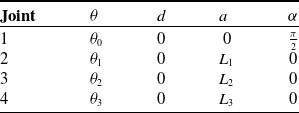
Forward kinematics computes the end-effector’s position and orientation from known joint angles and link lengths. We adopt the Denavit-Hartenberg (DH) convention, which provides a systematic method to describe the kinematic parameters of the robotic arm. These parameters are summarized in Table I.
By substituting the DH parameters into the transformation matrices, we can compute the position of the end-effector
 $X_4$
[Reference Nguyen, Phan, Vo, Trinh, Nguyen, Tran and Tran9]. Similarly, using the same approach, the positions of the other three joints,
 $X_1$
,
 $X_2$
, and
 $X_3$
, can also be determined.
2.2. Inverse kinematics
Given the coordinates
 $(x,y,z)$
of a point in space and the end-effector angle
 $\alpha$
between the manipulator’s end-effector and the horizontal plane, inverse kinematics determines the joint angles required to achieve a desired end-effector position and orientation, relying on geometric relationships [Reference Ting, Hairi, Zaman, Ibrahim and Moubark10, Reference Jazar11]. Due to the unique design of our manipulator, we can decompose the problem into a 3-DOF manipulator and an overall rotational motion.
For the overall rotation, the joint angle can be easily computed using geometric relationships from the top-down view.
DH table.

A 4-DOF Robotic arm,
 $\alpha$
in the figure is the end-effector angle.

For a 3-DOF planar robotic manipulator, the joint angles
 $\theta _1, \theta _2, \theta _3$
can be adjusted to position the end-effector
 $X_4$
at coordinates
 $(x,y,\alpha )$
.
 \begin{equation} \begin{cases} \displaystyle X_{3x}=X_{4x}-L_3\cos \alpha \\ \displaystyle X_{3y}=X_{4y}-L_3\sin \alpha \end{cases} \end{equation}
Since the position of
 $X_3$
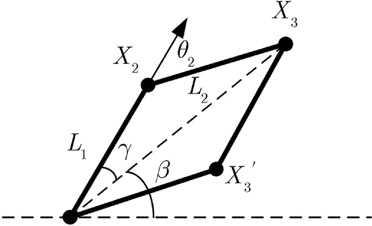
is determined, the problem can be further reduced. Thus, we simplify the planar 3-DOF robotic arm to a 2-DOF system, as illustrated in Figure 2.
2-DOF robot arm inverse kinematic. For the same 2D point, there are generally two solutions.

 \begin{equation} \begin{cases} \displaystyle \theta _1=\beta \pm \gamma \\[3pt] \displaystyle \tan \beta =\frac {X_{3y}}{X_{3x}} \\[8pt] \displaystyle \cos \theta _2=\frac {(X_{3y}^2+X_{3x}^2)-L_1^2-L_2^2}{2L_1L_2} \\[8pt] \displaystyle \cos \gamma =\frac {(X_{3y}^2+X_{3x}^2)+L_1^2-L_2^2}{2L_1\sqrt {X_{3y}^2+X_{3x}^2}}\\ \theta _3 = \alpha - \theta _1 - \theta _2 \end{cases} \end{equation}
These equations provide a means to calculate the joint angles
 $\theta _0, \theta _1, \theta _2,$
and
 $ \theta _3$
.
3. Bézier trajectory generation
Bézier curves exhibit excellent spatial continuity, making them highly effective for generating smooth spatial paths. By adjusting the control points, not only can the local velocity and acceleration be fine-tuned, but the overall shape of the curve can also be modified with high computational efficiency. The mathematical representation of an
 $ n$
-th degree Bézier curve is given by
 \begin{equation} f(t)=\sum _{i=0}^{n} B_i^{(n)}(t)\,\boldsymbol{p}_i = \sum _{i=0}^{n} \left({n\atop i}\right) t^i(1-t)^{n-i}\,\boldsymbol{p}_{i}, \end{equation}
 $ B_i^{(n)}(t)$
are the Bernstein basis polynomials, and
 $ \boldsymbol{p}_i$
are the control points. Then we can use the De Casteljau algorithm, which is commonly used to evaluate Bézier curves. This ensures numerical stability and provides a straightforward method for curve interpolation and refinement.
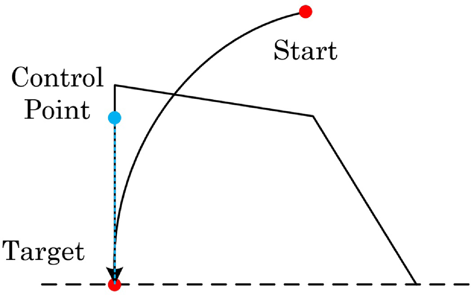
A schematic illustrating the path generated by the Bézier curve. The blue point is a control point that adjusts the curve’s final direction, while the red points mark the starting and ending positions.

We need to lay bricks one by one and ensure that they are placed as vertically as possible to utilize the mortise and tenon structure. This ensures that the bricks can fit together without colliding. So consider the following simplified scenario shown in Figure 3: the task of placing bricks from an initial position to a target location while ensuring that the trajectory remains vertically aligned at the end-effector, i.e., the end-effector remains perpendicular to the ground upon reaching the target point. To achieve this objective, we can utilize the tangent property of Bézier curves [Reference Jiao, Cao, Zhao, Liu and Tan12]. Specifically, a control point is added directly above the target point. By adjusting the distance
 $d$
between the control point and the target point, the shape of the trajectory can be manipulated to meet the desired alignment.
Given the need to solve for four joint angles, we have four degrees of freedom (DOF). With the known positions of
 $x$
,
 $y$
, and
 $z$
, three degrees of freedom can be determined. However,
 $\alpha$
remains to be selected.
4. Linear interpolation of the end-effector angle
Due to the change in
 $\alpha$
, which leads to changes in three joint angles, we aim to minimize the overall change rate of
 $\alpha$
while ensuring it remains within its feasible range. Mathematically, this can be expressed as:
 \begin{equation} \begin{aligned} &\text{minimize} \int _0^1 \left |\frac {d\alpha (t)}{dt}\right | dt \\ \text{subject to} \quad & \alpha _{\text{min}}(t) \leq \alpha (t) \leq \alpha _{\text{max}}(t), \quad \forall t \in [0,1]\\ \quad & \alpha (0) = \alpha _{\textrm { s}}, \quad \alpha (1) = \alpha _{\textrm { e}} \end{aligned} \end{equation}
 $\alpha (t)$
represents the angle
 $\alpha$
as a function of time
 $t$
, and
 $\alpha _{\text{min}}(t)$
and
 $\alpha _{\text{max}}(t)$
are the lower and upper bounds of the feasible range of
 $\alpha$
at time
 $t$
, respectively.
4.1. The end-effector angle’s bound
Based on (1), we can solve for the position of
 $X_3$
. Since
 $X_3$
is also a joint of the robotic arm, it must satisfy the length constraints of the first two links. Specifically, the distance from
 $X_3$
to the origin must be between
 $L_1-L_2$
and
 $L_1+L_2$
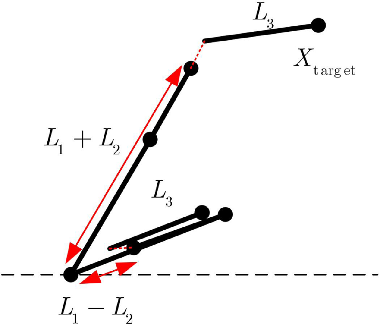
for a solution to exist. As shown in Figure 4, when the distance from to exceeds the allowable range, no solution exists.
The illustration of the case with no solution shows that the distance from
 $ X_3$
to
 $X_1$
is greater than
 $ \|L_1 + L_2\|$
or less than
 $ \|L_2 - L_1\|$
(highlighted in red in the diagram), indicating that this scenario cannot satisfy the length constraints of the links.

This can be described as a circle centered at
 $X_4$
with radius
 $L_3$
must overlap with an annular region centered at the origin with inner radius
 $L_1-L_2$
and outer radius
 $L_1+L_2$
. The
 $\alpha$
values corresponding to these overlapping points on the circle define the range of feasible angles. This constraint can be expressed by the following equation:
 \begin{equation} L_1-L_2 \leq \|X_3-X_1\| \leq L_1+L_2 \quad \text{and} \quad \|X_4-X_3\| = L_3 \end{equation}
 $\|X_3-X_1\|$
represents the distance from
 $X_3$
to the origin
 $X_1$
, and
 $\|X_4-X_3\|$
represents the distance between
 $X_4$
and
 $X_3$
.
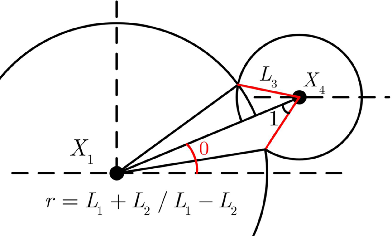
To determine the range of alpha values, assuming the two circles intersect, we can draw a diagram as shown in Figure 5. At this point, we need to calculate the alpha values corresponding to the two intersection points. As can be seen from the figure, the lengths of the three sides of the triangle are known. Therefore, we can calculate the three angles of the triangle. Subsequently, we can obtain several relationships from which we can derive the two alpha values, as follows:
Given that the three sides of the triangle are
 $\|X_4-X_1\|$
,
 $r$
and
 $L_3$
, we can solve for the three angles of the triangle. Let the angle between
 $X_4X_1$
and the X-axis be angle
 $\angle 0$
, and the angle between
 $X_4X_1$
and
 $L_3$
be
 $\angle 1$
.
The diagram for determining the range of
 $\alpha$
can be solved using
 $\angle 0$
, which is the angle between line segment
 $X_4X_1$
and the horizontal plane, along with the relationships of the triangle’s three sides. This allows for the calculation of the two
 $\alpha$
angles, which are indicated by red lines in the diagram.

Therefore, we can obtain two
 $\alpha$
values:
 \begin{equation} \begin{cases} \alpha _1 = \angle 0 + \angle 1 \\ \alpha _2 = \angle 0 - \angle 1 \end{cases} \end{equation}
Through numerical solution by sampling and the theoretical solution method described above, we obtained the range of feasible alpha values for
 $L_1=0.105\text{m},L_2=0.057\text{m},L_3=0.17\text{m}$
, which is illustrated in the following figure.
The blue area in the diagram represents the region where
 $\alpha$
has a solution. It can be observed that in this case, there is no trajectory such that the entire trajectory lies within the blue area; therefore, a continuous solution does not exist.

Here,
 $\alpha _1$
and
 $\alpha _2$
correspond to the case where
 $L_1 + L_2 = ||X_3||$
, while
 $\alpha{'}_1$
and
 $\alpha{'}_2$
correspond to the case where
 $L_1 - L_2 = ||X_3||$
.
4.2. Interpolation method
A straightforward method for determining
 $\alpha$
is through linear interpolation from the start value of
 $\alpha _{\text{s}}$
to the target value of
 $\alpha _{\text{e}}$
, as shown in Figure 6.
From the analysis above, we observe that in some cases, it is not always possible to continuously vary
 $\alpha$
from the initial value to the target value. For such situations, the simplest method is linear interpolation, but this does not ensure smooth slope transitions at the endpoints, leading to a very unsmooth curve. Therefore, we use Bézier or Hermite interpolation.
Compared to Hermite interpolation, Bézier curves offer more flexibility in shaping the curve by adjusting control points. This flexibility allows us to reduce significant deviations from the original path while maintaining a relatively simple and computationally efficient approach, while Hermite interpolation is more accurate and smoother [Reference Hashemi-Dehkordi and Valentini13].
However near elbow singularity configurations, the joint rates become unacceptably large, leading to large fluctuations in the interpolated curve [Reference Xu, Liang and Xu14]. To mitigate this, we revise the criteria for identifying unsolvable cases. As defined in (5) we introduce a discount factor
 $p$
and deem a trajectory point unsolvable when:
 \begin{equation} p\|X_3-X_1\| \leq (L_1-L_2) \quad \text{or} \quad \|X_3-X_1\| \geq p(L_1+L_2) \end{equation}
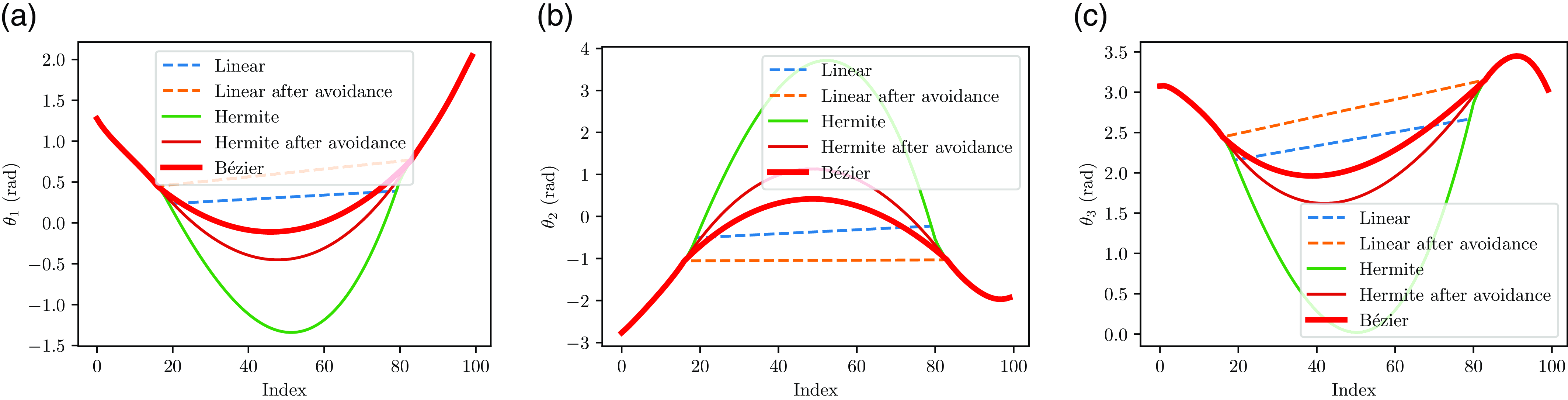
With this adjustment, we significantly reduce the occurrence of elbow singularities, and the interpolation results, as shown in Figure 7, demonstrate improved smoothness and accuracy.
This figure presents the results of the interpolation methods. The blue linear interpolation deviates significantly from the original trajectory and has unsmooth transitions. The green Hermite interpolation is smoothest but slightly deviates from the original path. The red Bézier interpolation is closer to the original trajectory while maintaining a good level of smoothness. (a) joint 1, (b) joint 2, (c) joint 3.

With this improvement, the overall trajectory follows the desired path in Cartesian space more accurately while maintaining smooth transitions. We present a comparative visualization in Figure 8.
The blue linear interpolation deviates significantly from the original trajectory and has unsmooth transitions. The green Hermite interpolation is smoothest but slightly deviates from the original path. The red Bézier interpolation is closer to the original trajectory while maintaining a good level of smoothness.

5. Planning as inference for end-effector angle
In most cases, it is possible to allow
 $\alpha$
to vary continuously from the initial value to the target value. During this process, the trajectory can be designed to avoid passing through regions where no solution exists so we can strictly follow the path. Therefore, the problem transforms into: assuming a feasible path exists, how to choose a path that minimizes the rate of change of
 $\alpha$
.
In this section, we will use probabilistic inference to choose the optimal alpha value. Generating alpha value could be considered as a process of generating a minimum change rate trajectory without collision. Considering the above two criteria, we can transform the problem into maximum a posteriori (MAP) estimation problem. Then we can generate the path by maximizing the conditional posterior distribution
 $p(\boldsymbol{\alpha }|\mathbf {X})$
[Reference Bari, Wang, Haidari and Wollherr15].
 \begin{equation} \begin{aligned} \hat {\boldsymbol{\alpha }}_{\mathrm{MAP}} &=\arg \max P(\boldsymbol{\alpha }|\mathbf {X}) \\ &=\arg \max P(\boldsymbol{\alpha }) P(\mathbf {X}|\boldsymbol{\alpha }) \end{aligned} \end{equation}
The first is the prior factor, and the second is the likelihood factor.
5.1. Define the factors
First, we consider the prior distribution of the alpha value. We need to make sure that the alpha value is always within the feasible range and can connect the start and endpoint. So we choose center line of the region as the prior path. For this problem, we notice that the boundary of the region may change from upper path to lower path or lower path to upper path, so when transitioning from one region to another, we use interpolation to generate the path.
Assume that the centerline changes from
 $\alpha _1$
to
 $\alpha _2$
as time
 $t$
progresses from
 $t_1$
to
 $t_2$
. In this case, we apply interpolation over the time interval
 $[t_1,t_2]$
, ensuring a smooth transition that respects the region boundaries.
 \begin{equation} \begin{cases} \displaystyle p=\frac {t-t_1}{t_2-t_1} \\ \displaystyle \alpha (t) = (1-p)\alpha _1 + p\alpha _2 \end{cases} \end{equation}
The interpolation sometimes may not be smooth, so we use savgol filter to smooth the path and then we get the prior path
 $\boldsymbol{\mu }$
.
But notice We haven’t make sure
 $\alpha (t_0) = \alpha_{\textrm{s}}, \; \alpha (t_N) = \alpha_{\textrm{e}}$
. So we need to make sure the path always satisfies this condition while MAP optimization.
To achieve this, we can define a Gaussian Process (GP) prior on the space of trajectories,
 $\boldsymbol{\alpha }(t) \sim (\boldsymbol{\mu }(t), {\mathbf {K}}(t, t'))$
, where
 $\boldsymbol{\mu }(t)$
is a mean function and
 ${\mathbf {K}}(t,t')$
is a covariance function. The GP is a collection of random variables, so we can use the covariance matrix to add constraints on the path. To facilitate the analysis, we discretize the path into
 $N$
points, i.e.,
 $\alpha _i = \alpha (t_i)$
, where
 $t_i = \frac {i}{N}$
. Therefore,
 $\boldsymbol{\alpha }$
has a joint Gaussian distribution:
 \begin{equation} {\boldsymbol{\alpha}} = \begin{bmatrix} \alpha _0 & \ldots & \alpha _N \end{bmatrix}^\top \sim {\mathcal{N}}({\boldsymbol {\mu}}, {\mathbf {K}}) \end{equation}
where the mean vector is
 $\boldsymbol{\mu }$
and the covariance kernel is
 ${\mathbf {K}}$
.
The GP defines a prior on the space of trajectories :
 \begin{align} p(\boldsymbol{\alpha }) &\propto \exp \bigg \{ - \frac {1}{2} \parallel \boldsymbol{\alpha } - \boldsymbol{\mu } \parallel ^{2}_{\mathbf {K}} \bigg \} \end{align}
where
 $\parallel \boldsymbol{\alpha } - \boldsymbol{\mu } \parallel ^{2}_{\mathbf {K}} \doteq (\boldsymbol{\alpha } - \boldsymbol{\mu })^\top {\mathbf {K}}^{-1} (\boldsymbol{\alpha } - \boldsymbol{\mu })$
.
For the boundary condition, we need to define a linear observation model
 $\mathbf{Y}$
[Reference Mukadam, Dong, Yan, Dellaert and Boots16].
 \begin{equation} {\mathbf {Y}} = C\boldsymbol{\alpha } + \epsilon, \quad \epsilon \sim {\mathcal {N}}(0, {\mathbf {K}}_y). \end{equation}
We can write their joint distribution as
 \begin{equation} {\mathcal {N}} \Bigg ( \left [ \begin{matrix} \boldsymbol{\mu } \\ C\boldsymbol{\mu } \end{matrix} \right ], \left [ \begin{matrix} {\mathbf {K}} & {\mathbf {K}}C^\top \\ C {\mathbf {K}} & C {\mathbf {K}}C^\top + {\mathbf {K}}_y \end{matrix}\right ] \Bigg ). \end{equation}
Conditioned on the observations, we can update the mean and covariance of the Gaussian Process as follows:
 \begin{equation} \boldsymbol{\mu } = \boldsymbol{\mu } + {\mathbf {K}}C^\top ({\mathbf {K}}C^\top + {\mathbf {K}}_y)^{-1} (\boldsymbol{\alpha } - C\boldsymbol{\mu }) \end{equation}
 \begin{equation} {\mathbf {K}} = {\mathbf {K}} - {\mathbf {K}}C^\top ({\mathbf {K}}C^\top + {\mathbf {K}}_y)^{-1}C{\mathbf {K}} =({\mathbf {K}}^{-1} + C^\top {\mathbf {K}}^{-1}_yC)^{-1} \end{equation}
Since we only need the observation at the start alpha
 ${\mathcal {N}}(\alpha _{\textrm { s}},K_{\textrm { s}})$
and endpoint
 ${\mathcal {N}}(\alpha _{\textrm { e}}, K_{\textrm { e}})$
, we can set
 $C_1 = [1, 0, \ldots, 0], C_2 = [0, \ldots, 0, 1]$
, substituting these into (14) (15) we get
 \begin{equation} \begin{aligned} \boldsymbol{\mu } &= \widetilde {\boldsymbol{\mu }} + {\mathbf {K}}C_1^\top ({\mathbf {K}}(t_0,t_0) + K_{\textrm { s}})^{-1} (\alpha _{\textrm { s}} - \widetilde {\boldsymbol{\mu }}(t_0))\\ &\quad +{\mathbf {K}}C_2^\top ({\mathbf {K}}(t_N,t_N) + K_{\textrm { e}})^{-1} (\alpha _{\textrm { e}} - \widetilde {\boldsymbol{\mu }}(t_N))\\ {\mathbf {K}} &= ({\mathbf {K}}^{-1} + C_1^\top K^{-1}_{\textrm { s}}C_1+C_2^\top K^{-1}_{\textrm { e}}C_2)^{-1} \end{aligned} \end{equation}
To ensure the smoothness of the path, we need to minimize the changes of the path, which can be expressed as
 \begin{equation} P(\mathbf{X}|\boldsymbol{\alpha }) \propto \exp \bigg \{ -\frac {1}{2}\sum _{i=1}^{N-1} \parallel \alpha _i - \alpha _{i+1}\parallel ^2 \bigg \} \end{equation}
5.2. Optimization
Combining the prior factor and the minimum changes factor using (8), we can get the posterior distribution of
 $\alpha$
. Here we use
 $\lambda$
to control the balance between the prior factor and likelihood factor.
 \begin{equation} P(\boldsymbol{\alpha }|\mathbf{X}) \propto \exp \bigg \{ - \frac {1}{2} \parallel \boldsymbol{\alpha } - \boldsymbol{\mu } \parallel ^2_{{\mathbf {K}}}-\frac {\lambda }{2}\sum _{i=1}^{N-1} \parallel \alpha _i - \alpha _{i+1}\parallel ^2 \bigg \} \end{equation}
We can take a negative log to transfer the problem into an optimization problem.
 \begin{equation} \hat {\boldsymbol{\alpha }}_{\mathrm{MAP}} = \arg \min \left [\parallel \boldsymbol{\alpha } - \boldsymbol{\mu } \parallel ^2_{{\mathbf {K}}} + \lambda \sum _{i=1}^{N-1} \parallel \alpha _i - \alpha _{i+1}\parallel ^2 \right ] \end{equation}
We can search the optimal
 $\lambda$
by increasing it from 0 to a large enough number while checking the path with a feasible solution. We use gradient-based optimizer to solve the optimization problem. The optimization result is shown in Figure 9.
The diagram of the optimization results shows that if interpolation is used, there exists a portion of
 $\alpha$
with no solution. However, by utilizing Gaussian processes for optimization, we first obtain the yellow centerline path and then apply boundary conditions to derive the blue prior path. Finally, we optimize the trajectory with different values of
 $\lambda$
to achieve the optimal values for
 $\alpha$
.

The algorithm to find the optimal path for the Bézier curve is outlined in Algorithm 1.
Find the Optimal Path for Bézier Curve

6. Result and discussion
6.1. Interpolate evaluation
By employing inverse kinematics to compute the joint angles of the robotic arm, we can subsequently derive the angular velocity, acceleration, and jerk of the arm based on these angles.
To evaluate the trajectory of the robotic arm, we propose a metric designed to assess energy consumption during pick-and-place tasks by minimizing the sum of the joint rates. Furthermore, it is crucial to ensure that abrupt variations in acceleration—whether positive or negative—are minimized to prevent excessive mechanical stress and potential damage to the robotic arm. In this context, jerk, defined as the third derivative of position, is widely used in research to evaluate such factors [Reference Ye, Hao and Cheng17, Reference Dobiš, Dekan, Beňo, Duchoň and Babinec18]. Building on these considerations, we introduce a composite metric that simultaneously accounts for both joint rates and joint jerks, thereby promoting energy efficiency and smooth motion.
Let
 $\theta _{i,j}$
denote the angle of the
 $i$
th joint at the
 $j$
th time step. To quantify energy efficiency, we employ the discrete absolute change in joint angles between consecutive time steps, represented as
 $||\theta _{i,j} - \theta _{i,j-1} ||$
, which serves as a time-parametrized measure of the trajectory. Additionally, the joint jerk, denoted as
 $\theta ^{(3)}_{i,j}$
, is incorporated to capture the impact of abrupt changes in acceleration. To ensure that both positive and negative jerk fluctuations are equally accounted for, we utilize the absolute value of the jerk. This prevents the underestimation of sudden acceleration changes that might otherwise be masked by cancelation effects. Integrating these components, we define the metric
 $E_1$
as follows:
 \begin{equation} E_1 = \sum _{i=1}^3 \sum _{j=1}^N \left \lVert (\theta _{i,j} - \theta _{i,j-1}) \theta ^{(3)}_{i,j} \right \rVert \end{equation}
This formulation effectively penalizes rapid fluctuations in acceleration while maintaining computational simplicity by avoiding intricate calculations. The use of absolute values ensures that both abrupt increases and decreases in acceleration contribute equally to the metric, thereby promoting smoother and more stable trajectories for the robotic arm. By minimizing
 $E_1$
, we can achieve trajectories that are not only energy-efficient but also mechanically sustainable, reducing wear and tear on the robotic system.
In addition, we define the metric
 $E_2$
as the sum of the distances between the original path and the interpolated path, calculated as follows:
 \begin{equation} E_2 = \sum _{j=1}^N||p^\prime _j-p_j|| \end{equation}
The results of our evaluation are summarized in Table II.
Evaluation results for different
 $p$
values and interpolation methods.

From the table, we observe that as the value of
 $p$
decreases, both metrics
 $E_1$
and
 $E_2$
generally decrease for all interpolation methods except
 $E_2$
in the linear method. This suggests that the linear method interpolates the path without accounting for boundary conditions, resulting in larger
 $E_2$
values as more trajectory points are interpolated. Hermite interpolation yields smoother trajectories with lower
 $E_1$
values compared to the other methods. This is particularly beneficial for applications requiring high precision and minimal abrupt changes in motion. On the other hand, Bézier curves allow for the adjustment of control point parameters, which helps to minimize deviations from the original trajectory while still maintaining a relatively smooth path. Ultimately, the choice between these methods can be made based on the specific needs of the task at hand.
6.2. Gaussian process optimization result
We plot the angles of each joint for different values of
 $\lambda$
, as shown in Figure 10.
Comparison of joint angles obtained using different values of
 $\lambda$
for optimization. As
 $\lambda$
increases, the curves become smoother, indicating improved trajectory quality. (a) joint 1, (b) joint 2, (c) joint 3.

To further test and visualize the algorithm’s results, we set up a surface simulation environment by importing a surface model, along with models of the robot car and bricks, based on Nvidia Isaac Sim and conducted simulation tests.
The left image shows the unoptimized trajectory of the brick, while the right image displays the optimized trajectory, which strictly follows the Bézier curve.

As shown in Figure 11, the optimized trajectory satisfies the end-effector constraints and is better suited for the pick-and-place task.
The two figures show the simulation results in the NVIDIA Isaac Sim environment. It can be observed that, except for slight oscillations at the beginning of the motion, the velocity remains stable at a relatively low value during the rest of the time. (a) linear velocity (b) angular velocity.

We obtained the linear velocity and angular velocity of the brick during placement and compared it with the result of linear interpolation of angles without considering the path. As shown in Figure 12, it can be seen that our method is very close to the smoothest possible change while ensuring path constraints, accomplishing the path planning task under the condition of minimizing the brick’s speed as much as possible.
7. Conclusion
This study presents a comprehensive approach to trajectory planning for a 4-DOF robotic arm. The algorithm framework includes two cases for trajectory planning: when a continuous solution does not exist and when it does. For the former, we propose a method to interpolate the path using Bézier or Hermite methods, while for the latter, we introduce a probabilistic inference approach to optimize the trajectory. Our method can generate a smooth trajectory that follows the Cartesian path as closely as possible while ensuring the end-effector angle remains within feasible limits. The results of our evaluation demonstrate that the proposed method can effectively generate a trajectory for pick-and-place tasks. Future work could explore integrating this method with better prior trajectories and further optimizing methods to ensure smoother joint angle transitions. Additionally, experimental validation on physical robotic systems would further demonstrate the practical benefits of this approach.
Author contributions
Shiwei Pan, Jiaxue Li, and Xiaoxiao Lv conducted the majority of the research and analysis. Shiwei Pan drafted the manuscript. Wenrui Jin provided guidance and supervision throughout the study.
Financial support
This work was supported by Construction of Plateau Discipline of Shanghai at Tongji University (grant no. 0200121005/180/005), Tongji University Interdisciplinary Joint Research Project (grant no. 2023-2-ZD-09 ) and Students Innovation Training Program of Tongji University (grant no. X2024150).
Conflicts of interest
The authors have no financial or proprietary interests in any material discussed in this article.
Ethical approval
None.