

1. Introduction
Flow control is either passive without power input or active with powered actuators, which can be of tremendous benefit in a number of applications (Gad-el Hak Reference Gad-el Hak2007). Typical examples include the altering and suppression of vortex shedding, enhanced mixing, drag reduction and noise abatement (Gad-el Hak, Pollard & Bonnet Reference Gad-el Hak, Pollard and Bonnet2003; Choi, Jeon & Kim Reference Choi, Jeon and Kim2008; Ceccio Reference Ceccio2010; Tan, Zhang & Lv Reference Tan, Zhang and Lv2018). In the last few decades efforts have been made to improve the ability of manipulating fluid dynamics. One of the foremost challenges in flow control is the placement of control devices, which is crucial to the performance of both passive control (Strykowski & Sreenivasan Reference Strykowski and Sreenivasan1990; Hwang & Choi Reference Hwang and Choi2006) and active control (Belson et al. Reference Belson, Semeraro, Rowley and Henningson2013). Finding the optimal placement for control devices, although challenging, could significantly improve the effectiveness and efficiency of flow control schemes and provide deeper insights into the physical properties of fluid flows.
1.1. Placement of control devices
Most studies concerning optimal placement are based on the physical characteristics of flow systems (Chomaz Reference Chomaz2005; Schmid & Brandt Reference Schmid and Brandt2014). Some recent studies have suggested that any sensors should be placed where any unstable eigenmodes are large for the best detectability for those modes, and that any actuators should be placed where the corresponding adjoint modes are large for the best stabilisability for those adjoint modes (Lauga & Bewley Reference Lauga and Bewley2003; Åkervik et al. Reference Åkervik, Hœpffner, Ehrenstein and Henningson2007; Bagheri et al. Reference Bagheri, Henningson, Hoepffner and Schmid2009). Similar arguments were also given based on a Gramian-based analysis of the open-loop system with full sensing and actuation: good sensor locations overlap with regions that have the largest response to external disturbances, as indicated by the leading eigenmodes of the controllability Gramian; good actuator locations overlap with regions that have the highest receptivity to perturbations, as indicated by the leading eigenmodes of the observability Gramian (Ma, Ahuja & Rowley Reference Ma, Ahuja and Rowley2011; Chen & Rowley Reference Chen and Rowley2014).
Moreover, Lauga & Bewley (Reference Lauga and Bewley2004) considered linear  $\mathcal {H}_{\infty }$ feedback control of the complex Ginzburg–Landau (CGL) equation and placed an actuator and a sensor in the wavemaker region, which was originally introduced for the case of weakly non-parallel flows (Chomaz, Huerre & Redekopp Reference Chomaz, Huerre and Redekopp1991; Monkewitz, Huerre & Chomaz Reference Monkewitz, Huerre and Chomaz1993). Further work conducted by Giannetti & Luchini (Reference Giannetti and Luchini2007) defined a wavemaker region using an eigenvalue sensitivity analysis for strongly non-parallel flows, e.g. the cylinder flow, based on the concept of localised feedback of flow perturbations. Specifically, these regions describe the overlap between any unstable eigenmodes and their corresponding adjoint eigenmodes, inside which local feedback mechanisms could result in large modifications of any unstable eigenvalues to push them into the stable half-plane. Based on this eigenvalue sensitivity analysis, Camarri & Iollo (Reference Camarri and Iollo2010) determined the types and positions of sensors as well as feedback coefficients for a simple proportional feedback control law for the flow past a square cylinder confined in a channel. Their strategy led to the successful stabilisation of the flow up to a Reynolds number that was 100 % higher than the critical value after which otherwise the flow would become unsteady. Similar studies have employed various sensitivity analyses for the selection and placement of collocated actuator–sensor pairs in a separated boundary layer (Natarajan, Freund & Bodony Reference Natarajan, Freund and Bodony2016) and optimal sensor placement for variational data assimilation of unsteady flows (Mons, Chassaing & Sagaut Reference Mons, Chassaing and Sagaut2017). Rather than control perturbations, Marquet, Sipp & Jacquin (Reference Marquet, Sipp and Jacquin2008) assumed a steady forcing for base-flow modifications and reproduced flow-stabilising regions using sensitivity analysis, which showed good agreement with those found experimentally by Strykowski & Sreenivasan (Reference Strykowski and Sreenivasan1990). A more detailed comparison between these studies is presented in Sipp et al. (Reference Sipp, Marquet, Meliga and Barbagallo2010).
Although the modal analyses described above provide sensible placements for control purposes, they do not yield the true optimal placement due to the strong non-normality of fluid flows. Therefore, a rigorous methodology and justification for finding the optimal placement should be based on the optimal control performance of each possible actuator–sensor configuration. Standard metrics of quantifying control performance include the  $\mathcal {H}_2$ norm which measures the energy of the system's impulse response and the
 $\mathcal {H}_{\infty }$ norm which measures the worst-case (i.e. most amplified) response to harmonic forcing (Skogestad & Postlethwaite Reference Skogestad and Postlethwaite2007, pp. 368–382). However, it is challenging to recompute the optimal control performance for each new placement of sensors and actuators, especially for high-dimensional control problems arising from two- or three-dimensional flows. Lauga & Bewley (Reference Lauga and Bewley2003) considered the one-dimensional Ginzburg–Landau system for which a full-state information controller (i.e. linear quadratic regulator) was designed for each possible actuator position. The variation of the optimal actuator location with Reynolds number was compared with that predicted by eigenanalysis. Recent studies have also considered optimal sensor placement for state estimation of the one-dimensional dispersive wave equation (Khan, Morris & Stastna Reference Khan, Morris and Stastna2015) and the Boussinesq equations that model a controlled thermal fluid (Hu, Morris & Zhang Reference Hu, Morris and Zhang2016). Reduced-order modelling has also been employed in optimal placement problems for two-dimensional flows, such as the flow over a backward-facing step (Juillet, Schmid & Huerre Reference Juillet, Schmid and Huerre2013) and the cylinder flow (Akhtar et al. Reference Akhtar, Borggaard, Burns, Imtiaz and Zietsman2015; Jin, Illingworth & Sandberg Reference Jin, Illingworth and Sandberg2020).
There are only few studies that rigorously analyse the optimal placements of sensors and actuators and their implications for the flow's closed-loop dynamics. Chen & Rowley (Reference Chen and Rowley2011, Reference Chen and Rowley2014) studied the optimal placement problem for  $\mathcal {H}_2$ optimal control of the CGL equation. They found the optimal sensor and actuator positions using an extended gradient minimisation algorithm developed by Hiramoto, Doki & Obinata (Reference Hiramoto, Doki and Obinata2000) for closed-loop control set-ups. In particular, the optimal placements of a single sensor and a single actuator were compared with those predicted by modal analyses, which demonstrated the shortcomings of eigenmode analysis and Gramian-based analysis for predicting optimal placements. Chen & Rowley (Reference Chen and Rowley2011) comment that these shortcomings are caused either by the strong non-normality of the system characterised by non-orthogonal eigenmodes or by the presence of time delays. They further comment that the wavemaker region proposed by Giannetti & Luchini (Reference Giannetti and Luchini2007), which indicates areas of high dynamical sensitivity, provides improved estimates of the optimal actuator and sensor placements. Oehler & Illingworth (Reference Oehler and Illingworth2018) further investigated optimal actuator and sensor placements for the same system but over a wider range of stability parameters. Their results indicated that the wavemaker region has no special significance for optimal placement and that, with increasing instability, the optimal placements move further away from that predicted by the wavemaker region. Instead, the optimal sensor and actuator positions show good agreement with those computed from the optimal estimation and full-state information control problems. A recent study of Jin et al. (Reference Jin, Illingworth and Sandberg2020) investigated optimal sensor placement in the two-dimensional cylinder wake using resolvent-based model-order reduction. A fundamental trade-off was demonstrated between measuring downstream information and reducing the time lag with respect to the actuator upstream. However, it is still not well understood whether feedback control performance is limited predominantly by the measurements (e.g. sensor placement) or by the actuation (e.g. actuator placement) or by their interaction in the overall feedback loop.
1.2. Objectives of the present work
The current work focuses on the optimal sensor and actuator placements for feedback control of the two-dimensional cylinder flow and investigates any trade-offs and coupling effects in the optimal placements. In this study we consider a velocity sensor that measures the perturbation velocity and an in-flow actuator that couples with the momentum of the flow and can be modelled as a body force. Similar control set-ups have been either numerically or experimentally investigated in many previous studies concerning the wake control behind bluff bodies. One typical example is passive control using a small control cylinder that was numerically modelled as an external forcing for sensitivity analysis (Marquet et al. Reference Marquet, Sipp and Jacquin2008). They successfully predicted the stabilisation zones for the cylinder flow that was experimentally found by Strykowski and Sreenivasan (Strykowski & Sreenivasan Reference Strykowski and Sreenivasan1990). The concept of a wavemaker region was defined based on the structural sensitivity analysis which theoretically predicts the optimal placement for the localised feedback (e.g. a local volume force) of flow perturbations (Giannetti & Luchini Reference Giannetti and Luchini2007). Other examples involve placing hot-wire sensors for off-body measurement (Roussopoulos Reference Roussopoulos1993; Gerhard et al. Reference Gerhard, Pastoor, King, Noack, Dillmann, Morzynski and Tadmor2003), using electrohydrodynamic devices or plasma actuators in the near wake to form a direct momentum transfer through a local body force (e.g. a Lorentz force) (Gerhard et al. Reference Gerhard, Pastoor, King, Noack, Dillmann, Morzynski and Tadmor2003; Hyun & Chun Reference Hyun and Chun2003; Deylami et al. Reference Deylami, Amanifard, Hosseininezhad and Dolati2017).
We first consider three optimal placement problems: (i) the optimal estimation (OE) problem in which the objective is to estimate the entire flow using a single sensor; (ii) the full-state information control (FIC) problem in which the entire flow field is known but only a single actuator is available for control; and (iii) the collocated input–output control (CIOC) problem in which a single sensor is available for measurements, which is collocated with a single actuator for control (localised feedback). By varying the Reynolds number and, therefore, the stability of the flow, any fundamental limitations or trade-offs are made clear for the optimal placements of a single sensor (OE), of a single actuator (FIC) and for localised feedback (CIOC).
The optimal performance achieved in the above three problems are compared with those achieved in the overall feedback control problem where a single sensor and a single actuator are separately placed at (i) the optimal positions found for the OE and FIC problems, respectively; and (ii) the optimal positions found for the overall feedback control problem. This provides a benchmark for evaluating the extent to which the optimal placements for the OE, FIC and CIOC problems approximate the optimal feedback control set-up and reveals any key factors that limit control performance. We discuss implications for sensor placement, actuator placement and the coupling effect between sensing and actuation (i.e. the time lag) for effective feedback control using a single sensor and a single actuator.
The work is organised as follows. Mathematical formulations and flow configurations are given in § 2. Arrangements and design method of the estimation and control problems are introduced in § 3. In § 4 we present results and discussions about the optimal sensor and actuator placements for feedback control of the two-dimensional cylinder flow. Conclusions are drawn in § 5.
2. Mathematical formulation
2.1. Governing equations
We consider the incompressible flow past a two-dimensional circular cylinder. The incompressible Navier–Stokes equations describe the conservation of mass and momentum of an incompressible fluid,
 \begin{equation} \left.\begin{gathered} \partial_t{\boldsymbol{u}}={-}{\boldsymbol{u}}\boldsymbol{\cdot} \boldsymbol{\nabla}{\boldsymbol{u}}- \boldsymbol{\nabla}\textit{p}+{\textit{Re}}^{{-}1} \nabla^2{\boldsymbol{u}},\\ \boldsymbol{\nabla}\boldsymbol{\cdot}{\boldsymbol{u}}=0, \end{gathered}\right\} \end{equation}
where the Reynolds number  ${\textit {Re}}={\textit {U}_{\infty }D}/{\nu }$ is based on a uniform inflow velocity
 $\textit {U}_{\infty }$ and the cylinder diameter
 $D$ to make all variables dimensionless. Here,
 $\nu$ is the kinematic viscosity. In this study we focus on Reynolds numbers in the range
 ${\textit {Re}} \in [50,\ 110]$ for which the cylinder wake has a single linearly unstable mode that drives the flow to periodic self-sustained limit-cycle oscillations (vortex shedding).
Note that the flow is asymptotically time periodic and two dimensional for  $Re$ up to approximately 188, where the flow becomes three dimensional (Barkley & Henderson Reference Barkley and Henderson1996; Williamson Reference Williamson1996; Barkley Reference Barkley2006). That is, the cylinder wake remains two dimensional for all Reynolds numbers considered in the study.
The objective of feedback control is to completely suppress vortex shedding behind a two-dimensional circular cylinder and drive the flow towards its unstable steady state (base flow). Therefore, we linearise the nonlinear Navier–Stokes equations (2.1) about the laminar base flow ( ${\boldsymbol {U}},\ \textit {P}$) which allows us to use existing linear control theory and analysis techniques,
 \begin{equation} \left.\begin{gathered} \partial_t{\boldsymbol{u}}'=\mathcal{L}{\boldsymbol{u}}'- \boldsymbol{\nabla}\textit{p}'+{\boldsymbol{f}}',\\ \boldsymbol{\nabla}\boldsymbol{\cdot}{\boldsymbol{u}}'=0. \end{gathered}\right\} \end{equation}
The perturbations ( ${\boldsymbol {u}}',\ \textit {p}'$) evolve according to the linear operator
 $\mathcal {L} = {-{\boldsymbol {U}}\boldsymbol {\cdot }\boldsymbol {\nabla }()} - {()\boldsymbol {\cdot }\boldsymbol {\nabla }{\boldsymbol {U}}} + {{\textit {Re}}^{-1}\nabla ^2()}$. The remaining nonlinear terms
 ${-{\boldsymbol {u}}'\boldsymbol {\cdot }\boldsymbol {\nabla }{\boldsymbol {u}}'}$ are neglected due to the assumption of small perturbations and the source term
 ${\boldsymbol {f}}'$ models any external forcing, such as stochastic disturbances or actuation. The linear perturbation equations (2.2) can also be written compactly as
 \begin{equation} \frac{\partial}{\partial t} \underbrace{\begin{bmatrix} \text{I} & \text{0}\\ \text{0} & \text{0} \end{bmatrix}}_{\mathcal{E}} \begin{bmatrix} {\boldsymbol{u}}'\\ \textit{p}' \end{bmatrix}=\underbrace{\begin{bmatrix} \mathcal{L} & -\boldsymbol{\nabla}()\\ -\boldsymbol{\nabla}\boldsymbol{\cdot}() & 0 \end{bmatrix}}_{\mathcal{A}} \begin{bmatrix} {\boldsymbol{u}}'\\ \textit{p}' \end{bmatrix}+ \underbrace{\begin{bmatrix} \text{I}\\ \text{0} \end{bmatrix}}_{\mathcal{P}}{\boldsymbol{f}}', \end{equation}
where  $\mathcal {E}=\mathcal {P}\mathcal {P}^T$ and
 $\mathcal {P}$ is the prolongation operator that maps a velocity vector
 ${\boldsymbol {u}}'$ to a velocity-zero-pressure vector
 $[{\boldsymbol {u}}',\ \text {0}]^T$;
 $\mathcal {A}$ denotes the linearized Navier–Stokes operator around the base flow.
2.2. Flow configuration and discretisation
The schematic diagram of the set-up used for the two-dimensional cylinder flow is displayed in figure 1, in which we employ the same computational domain and boundary conditions as those used by Leontini et al. (Reference Leontini, Stewart, Thompson and Hourigan2006) and Jin et al. (Reference Jin, Illingworth and Sandberg2020). A uniform free-stream velocity ( $\textit {U}_{\infty }=1$) is imposed at the inlet boundary (
 $\varGamma _{in}$) and encounters a cylinder (
 $\varGamma _{wall}$) of diameter
 $D=1$ with no-slip boundary conditions. Symmetric boundary conditions and standard outflow boundary conditions are imposed at the top boundary (
 $\varGamma _{top}$) and the outlet boundary (
 $\varGamma _{out}$), respectively. Note that the linear perturbation system has the same boundary conditions as those depicted in the figure except at the inlet where homogeneous boundary conditions (
 ${\boldsymbol {u}}'=[0,\ 0]$) are enforced to ensure zero perturbations at infinity.
Computational domain and boundary conditions for the cylinder flow (only a one-half-segment of the entire geometry is shown).

The Navier–Stokes equations are discretized using Taylor–Hood finite elements over a structured mesh using the FEniCS platform (Logg, Mardal & Wells Reference Logg, Mardal and Wells2012). The mesh points are clustered smoothly near the cylinder and in the wake to appropriately resolve the details of the flow. In particular, the mesh consists of  $2.7\times 10^4$ triangles and the minimum wall-normal spacing around the cylinder is 0.01. The compound state vector
 ${\boldsymbol {w}}=[{\boldsymbol {u}}',\ \textit {p}']^T\in \mathbb {R}^{N}$ thus has over
 $N=1.2\times 10^5$ degrees of freedom. The laminar base flow governed by the steady Navier–Stokes equations is then solved for using a Newton method. We use a backward Euler scheme for time discretization (
 $\Delta t=0.01$) in numerical simulations of the linear perturbation system. Mean (time-averaged) flow quantities are obtained by averaging results over 600 vortex shedding periods after the controlled flow is fully developed. This corresponds to a time horizon of around 5000 non-dimensional time units. Note that the laminar base flows and discretised perturbation systems have been validated by comparing them with the stability analysis results of Barkley (Reference Barkley2006). A sparse direct LU solver (MUMPS, Amestoy et al. Reference Amestoy, Duff, L'Excellent and Koster2001) and iterative Arnoldi methods (ARPACK, Lehoucq, Sorensen & Yang Reference Lehoucq, Sorensen and Yang1998) are used for all linear problems encountered in the study.
3. Modelling and control methods
We now consider the feedback control of linear perturbations in the flow. This section is organised as follows. The discretised input–output system is formulated in § 3.1. The estimation and control arrangements are then presented in § 3.2. In § 3.3 we introduce a resolvent-based design approach for the estimation and control problems.
3.1. Input–output system
The linear system (2.3) is subject to stochastic disturbances and actuation, which serve as perturbations and control mechanisms for the flow. Following spatial discretization, we can express (2.3) as a linear time-invariant state-space model  $\boldsymbol {P}(s)$ with outputs of interest (i.e.
 ${\boldsymbol {y}}$ and
 ${\boldsymbol {z}}$), as depicted in figure 2,
 \begin{equation} \left.\begin{gathered}
\boldsymbol{E}{{\boldsymbol{\dot {w}}}}=\boldsymbol{A}{\boldsymbol{w}}+\boldsymbol{B}_q{\boldsymbol{q}}+
\boldsymbol{B}_d{\boldsymbol{d},}\\
{\boldsymbol{y}}=\boldsymbol{C}_y{\boldsymbol{w}}+\boldsymbol{V}
{^{1/2}}
{\boldsymbol{n}},\\
{\boldsymbol{z}}=[\boldsymbol{C}_z{\boldsymbol{w}}\quad
\boldsymbol{R}^{1/2}{\boldsymbol{q}}]^T,
\end{gathered}\right\} \end{equation}
where the compound state vector  ${\boldsymbol {w}}=[{\boldsymbol {u}}',\ \textit {p}']^T$ and the matrix
 $\boldsymbol {E}=\boldsymbol {P}\boldsymbol {M}\boldsymbol {P}^T$. Here,
 $\boldsymbol {P}$ and
 $\boldsymbol {M}$ denote the prolongation matrix and the mass matrix of the velocity state due to the spatial discretization. The spatial discretization of actuation and statistical properties of disturbances are represented by the matrices
 $\boldsymbol {B}_q$ and
 $\boldsymbol {B}_d$, respectively. The disturbances are modelled as uncorrelated zero-mean Gaussian white noise and are injected over the entire velocity field. Therefore, the statistical properties of disturbances is given by
 $\boldsymbol {B}_d=\boldsymbol {P}\boldsymbol {M}^{1/2}$ after the spatial discretization (Croci et al. Reference Croci, Giles, Rognes and Farrell2018).
Block diagram of the state-space model (3.1), which is denoted as a transfer function  $\boldsymbol {P}(s)$ with the Laplace variable
 $s$.

The sensor measurement  ${\boldsymbol {y}}$ provides sensing and is characterised by the matrix
 $\boldsymbol {C}_y$. It includes a contribution from sensor noise
 ${\boldsymbol {n}}$ which is white in space and time with magnitude
 $\alpha$ (i.e.
 $\boldsymbol {V}^{1/2}=\alpha \boldsymbol {I}$). We aim to minimise the mean kinetic energy of linear perturbations
 ${\boldsymbol {w}}$. That is, the
 $\mathcal {H}_2$ norm of the performance measure
 ${\boldsymbol {z}}$ is minimised (with
 $\boldsymbol {C}_z=\boldsymbol {M}^{1/2}\boldsymbol {P}^T$). Therefore, the cost function is of the form
 \begin{equation} {\boldsymbol{J}}=\lim_{t\rightarrow\infty}\frac{1}{T}\int_0^T{\boldsymbol{z}}^T{\boldsymbol{z}}\,\textrm{d} t. \end{equation}
Note that the actuation input  ${\boldsymbol {q}}$ is a signal of interest in the control problem, which is scaled by
 $\beta$ to ensure that the control effort is sensible (i.e.
 $\boldsymbol {R}^{1/2}=\beta \boldsymbol {I}$).
3.2. Estimation and control set-ups
We employ  $\mathcal {H}_2$-optimal control tools as established by Doyle et al. (Reference Doyle, Glover, Khargonekar and Francis1988) to solve the feedback control (i.e. input–output control) problem for the linear system (3.1). A complete introduction to the method can be found in Skogestad & Postlethwaite (Reference Skogestad and Postlethwaite2007), in which any input–output control (IOC) problem is composed of two basic problems: (i) an OE problem and (ii) a FIC problem.
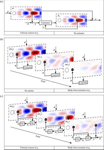
Detailed below and in Figure 3 are the three set-ups for the estimation and control problems considered.
(i) The OE problem, where the entire flow field is estimated using a single sensor that measures the perturbation velocity
 ${\boldsymbol {u}}'({\boldsymbol {x}}_s,t)$ at a single point in the flow. The sensor is contaminated by noise ${\boldsymbol {n}}$ of magnitude $\alpha =10^{-4}$ so that sensor noise is present but relatively small. For each sensor placement, we aim to minimise the mean (i.e. time-averaged) kinetic energy of the estimation error (${\boldsymbol {e}}={\boldsymbol {w}}-{\boldsymbol {w}}_e$) under the excitation of stochastic disturbances and in the presence of sensor noise. The optimal sensor position therefore leads to the smallest possible $\mathcal {H}_2$ norm of the estimation error (i.e. the OE of the entire cylinder flow).
(ii) The FIC problem, where the entire flow field is known (i.e. measured perfectly everywhere without any sensor noise
$\alpha =0$) but only a single body force ${\boldsymbol {f}}'({\boldsymbol {x}}_a,t)$ that serves as an in-flow actuator is available for control and operates according to the signal ${\boldsymbol {q}}$. For each actuator placement, the task of the FIC problem is to use a sensible control effort to minimise the mean kinetic energy of flow perturbations that are excited by stochastic disturbances. We choose a small control penalty of $\beta =10^{-4}$ to allow for relatively aggressive control. Analogous to the OE problem, the optimal actuator position achieves the smallest possible $\mathcal {H}_2$ norm of the perturbation velocity (i.e. the optimal FIC of the entire cylinder flow).(iii) The CIOC problem, where a single collocated actuator–sensor pair is available for both control and measurement (i.e.
${\boldsymbol {x}}_s={\boldsymbol {x}}_a$). In this case, we use the same set-ups as those used for the OE and FIC problems (i.e. $\alpha =\beta =10^{-4}$) but the single sensor and single actuator are collocated to model a localised feedback control mechanism with minimal time lag. For each collocated actuator–sensor placement, we aim to minimise the mean kinetic energy of flow perturbations under excitation from external disturbances and in the presence of sensor noise. The optimal position for the collocated actuator–sensor pair thus provides the best compromise between adequate estimation of the entire flow and adequate FIC of the entire flow.(iv) The general IOC problem, which shares the same set-up as that described in the CIOC problem but which uses a single sensor placed downstream for measurement and a single actuator placed upstream for control (i.e.
${\boldsymbol {x}}_s\neq {\boldsymbol {x}}_a$). In particular, we consider the sensor and actuator placements at i) the optimal positions that achieve the best feedback control performance; and ii) the optimal locations found for the OE and FIC problems, respectively. In the latter case, the sensor and actuator placements provide the best estimation performance and the best FIC performance, respectively, of the whole cylinder flow but may allow excessive time lag between the sensor and the actuator. By comparing it to the above three problems, we aim to evaluate the coupling effect between sensing and actuating, e.g. the time-lag effect, for effective feedback control.


Set-ups of the OE, FIC and IOC/CIOC problems. (a) Optimal estimation of the whole flow field using a single sensor at  ${\boldsymbol {x}}_s$. (b) Full-state information control using a single actuator at
 ${\boldsymbol {x}}_a$ when the entire flow field is known. (c) Input–output feedback control with a single sensor at
 ${\boldsymbol {x}}_s$ and a single actuator at
 ${\boldsymbol {x}}_a$.

Having defined the estimation and control set-ups, we then need to solve the OE and FIC problems (e.g. solve their corresponding Riccati equations). Based on the separation theorem (Georgiou & Lindquist Reference Georgiou and Lindquist2013), any IOC problem can be solved by combining the solutions of the corresponding OE and FIC problems. Refer to Appendix A for a summary of the systems and solutions for these problems. However, the generalized algebraic Riccati equations associated with the OE and FIC problems are generally of high dimension. Although it is common to perform numerical simulations for two- or three-dimensional fluid flows (i.e.  $N>10^5$), traditional control design tools (e.g. Riccati solvers) typically become computationally intractable for
 $N>10^3$. This difficulty has been partially overcome by a sparse Riccati solver using an extended low-rank method, in which the number of inputs and outputs (so-called terminals) is limited to be far less than the dimension of the control problem (Benner, Köhler & Saak Reference Benner, Köhler and Saak2019; Saak, Köhler & Benner Reference Saak, Köhler and Benner2019). For problems with either many inputs (e.g. full-state disturbances in the OE problem) or many outputs (e.g. full-state measuring in the FIC problem), no efficient numerical tools are available to directly handle large-scale systems. In the next section we will introduce a ‘terminal reduction’ method to overcome the challenges of many inputs and outputs.
3.3. Optimal estimator and controller design
As depicted in figure 5, the closed-loop transfer function  $\boldsymbol {G}(s)$ can be formed once the estimator or controller is designed, defined such that
 ${\boldsymbol {z}}=\boldsymbol {G}(s)[{\boldsymbol {d}},{\boldsymbol {n}}]^T$. The feedback law from the sensor measurement
 ${\boldsymbol {y}}$ to the actuation signal
 ${\boldsymbol {q}}$ is represented by the transfer function
 $\boldsymbol {Q}(s)$. For both the OE and FIC problems, our purpose is to minimise
 $\boldsymbol {G}(s)$ such that the performance measurement
 ${\boldsymbol {z}}$ is small. Therefore, an equivalent form of the cost function (3.2) is the
 $\mathcal {H}_2$ norm of
 $\boldsymbol {G}(s)$,
 \begin{align} {\boldsymbol{J}}=\lVert{\boldsymbol{G}(s)}\rVert^2_2&=\frac{1}{2{\rm \pi}}\int_{-\infty}^{\infty}
\text{tr}\{\boldsymbol{G}^H(\kern0.06em j\omega)\boldsymbol{G}(\kern0.06em j\omega)\}\,\textrm{d}\omega
\nonumber\\
&=\frac{1}{2{\rm \pi}}\int_{-\infty}^{\infty}\sum_{i}^{}\sigma^2_i(\kern0.06em j\omega)\,\textrm{d}\omega,
\end{align}
where  $\sigma _i(\kern0.06em j\omega )$ are the singular values of the transfer function
 $\boldsymbol {G}(s)$ at frequency
 $\omega$ arranged in descending order. The singular values of a transfer function can be considered as energy gains between a series of inputs and the corresponding outputs. We thus aim to minimise the integrated energy gain (3.3) for inputs and outputs over all frequencies and all possible directions.
However, it is not feasible to consider all inputs or outputs while designing estimators or controllers for a high-dimensional flow system. One possible solution is to consider an alternative cost function  $\gamma ^2{(k,\omega _n)}$ which only includes a limited number of singular values within a specified frequency range,
 \begin{equation} \gamma^2(k,\omega_n)=\frac{1}{2{\rm \pi}}\int_{-\omega_n}^{\omega_n}\sum_{i=1}^{k}\sigma^2_i(\kern0.06em j\omega)\,\textrm{d}\omega. \end{equation}
Therefore, only the first  $k$ orthogonal inputs and outputs across a limited frequency range
 $\omega \in [-\omega _n,\ \omega _n]$ will be considered. This cost function is constructed based on two insights: (i) for fluid flows, only a limited number of dominant physical mechanisms occur within a finite frequency range, e.g. the instability of the linearised cylinder flow occurs around
 $\omega _c\approx 0.8$; (ii) these physical mechanisms can be approximated by a small number of orthogonal inputs and outputs that have large energy gains
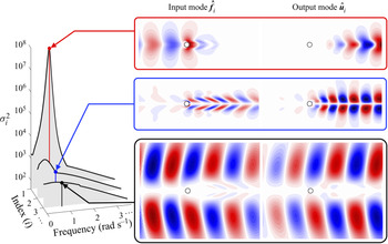
 $\sigma _i^2$, which are also the most significant for estimation or control. These can be more clearly seen in figure 4 where the first three energy spectra (i.e. singular values
 $\sigma ^2_i(\kern0.06em j\omega )$) are shown for the cylinder flow at
 ${\textit {Re}}=90$ together with the corresponding input and output modes at the unstable frequency
 $\omega \approx 0.76$. The first two output modes correspond to vortex shedding. In particular, the leading output mode
 $\hat {{\boldsymbol {u}}}_1$ corresponds to the amplification of upstream inputs
 $\hat {{\boldsymbol {f}}}_1$ while the second output mode corresponds to a local amplification of disturbances. The third output mode, however, consists of waves that are concentrated in the free stream. There exists a large separation between the first and other energy gains and we might expect that the physical mechanisms represented by the first few input and output modes are the most important for estimation and control. Instead of minimising all energy gains over all frequencies and all possible directions, it is more feasible to use the alternative cost function (3.4) that considers a significantly smaller number of inputs and outputs.
Resolvent analysis of the cylinder flow at  ${\textit {Re}}=90$. The first three energy spectra (
 $\sigma _i^2$) and the corresponding optimal input and output modes (transverse component, real part) at the unstable frequency
 $\omega \approx 0.76$ are shown (Jin, Illingworth & Sandberg Reference Jin, Illingworth and Sandberg2021).

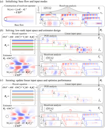
The implementation of the alternative cost function is depicted in figure 5, where we iteratively replace  $\boldsymbol {B}_d$ and
 $\boldsymbol {C}_z$ with properly constructed low-rank matrices (i.e.
 $\boldsymbol {B}_d=\boldsymbol {P}\boldsymbol {M}\tilde {\boldsymbol {F}}_m$ and
 $\boldsymbol {C}_z=\tilde {\boldsymbol {U}}_m\boldsymbol {M}\boldsymbol {P}^T$). In this case, the white noise disturbances applied everywhere are limited to orthonormal modes in the low-rank input basis
 $\tilde {\boldsymbol {F}}_m$. As for the full-state performance measure
 ${\boldsymbol {z}}$, the system states
 ${\boldsymbol {w}}$ are recast as linear combinations of orthonormal output modes in the low-rank output basis
 $\tilde {\boldsymbol {U}}_m$. Therefore, the number of either inputs or outputs is reduced to
 $m$ – the rank of the input and output bases. The construction of low-rank bases is based on the proper orthogonal decomposition (POD) of the first
 $k$ resolvent modes across a wide frequency range
 $[-\omega _n,\ \omega _n]$, which generates orthonormal POD modes ranked by their importance (i.e. the energy gain). In this study the low-rank bases
 $\tilde {\boldsymbol {F}}_m$ and
 $\tilde {\boldsymbol {U}}_m$ contain the first
 $m$ POD modes such that all relevant resolvent input and output modes can be recovered from linear combinations of orthonormal POD modes within a relative mismatch less than
 $10^{-6}$. Refer to Appendix B for more details concerning the implementation of the control design method. Note that resolvent analysis preferentially displays low-rank characteristics for physical mechanisms that are active in fluid flows (McKeon & Sharma Reference McKeon and Sharma2010; Sipp & Marquet Reference Sipp and Marquet2013). In other words, there often exists a large separation between singular values
 $\sigma _i$ such that only a limited number of forcing modes give rise to energetic responses that are the most important for estimation and control. By choosing a sufficient number of resolvent modes over a sufficiently large frequency range, the resulting performance should eventually converge to the true global optimum. In this study, we choose the parameter combination
 $k=3$ and
 $\omega _n=9$, which is sufficient to achieve convergence for both the optimal performance and the optimal placements (see Appendix C).
Schematic of the resolvent-based design approach for the optimal estimation and control of a high-dimensional flow system. The state-space model (3.1) is denoted as  $\boldsymbol {P}(s)$ and the closed-loop
 $\boldsymbol {G}(s)$ is formed by coupling the secondary transfer function
 $\boldsymbol {R}(s)$ from the sensor measurement
 ${\boldsymbol {y}}$ to the control signal
 ${\boldsymbol {q}}$.

4. Results
We now design optimal estimators and controllers for the two-dimensional cylinder flow and find the optimal sensor and actuator placements. This section consists of three parts: (i) the OE problem with a single sensor (figure 3a); (ii) the FIC problem with a single actuator (figure 3b); (iii) the CIOC problem with a single collocated actuator–sensor pair (figure 3(c) with  ${\boldsymbol {x}}_s={\boldsymbol {x}}_a$). In the last subsection, § 4.4, we further consider an IOC set-up with a single sensor and a single actuator placed at the optimal positions found for the OE and FIC problems, respectively (figure 3(c) with
 ${\boldsymbol {x}}_s\neq {\boldsymbol {x}}_a$). The comparison of the optimal performance among all four cases provides deeper insights into the sensor and actuator placement problems and the influence of their coupling for effective feedback control.
4.1. Optimal estimation problem
4.1.1. Brute-force sampling
To fully understand the effect of sensor placement, we start by performing a brute-force sampling approach for the OE problem at two Reynolds numbers:  ${\textit {Re}}=60$ and
 ${\textit {Re}}=110$. The OE problem is solved by implementing the method introduced in § 3 with parameters
 $k=3,\ \omega _n=9$. The corresponding cost function (3.4) is mapped out as a function of the sensor location (
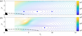
 $x_{s},\ y_{s}$) in figure 6. As discussed in § 3.3, the cost function
 $\gamma _{(k,\omega _n)}^2$, though excluding the contribution from ‘background’ modes, is sufficient to characterise the optimal estimator performance when random disturbances are applied everywhere and, thus, to determine the global optimal sensor location.
Contours of the cost function  $\gamma ^2{(k,\omega _n)}$ in the OE problem and the optimal sensor locations (
 $\bullet$, blue) at (a)
 ${\textit {Re}}=60$ and (b)
 ${\textit {Re}}=110$. The square (
 $\blacksquare$, blue) and triangle (
 $\blacktriangle$, blue) correspond to the sensor locations considered in figure 7. Estimators are designed using the parameters
 $k=3$ and
 $\omega _n=9$. The dash–dotted line (–
 $\cdot$ –) indicates the boundary of the reverse-flow region.

Some critical features are immediately seen in figure 6. First of all, the global optimal sensor location ( $\bullet$, blue) is at approximately
 $(x_s, y_s)=(6.83,\ 0.73)$ for
 ${\textit {Re}}=60$ and at
 $(x_s, y_s)=(8.41,\ 0.73)$ for
 ${\textit {Re}}=110$. The optimal sensor location therefore moves downstream with increasing Reynolds number but its transverse position remains constant. Second, at the lower Reynolds number (
 ${\textit {Re}}=60$), only one minimum exists. Although multiple extrema (maxima and minima) arise at the higher Reynolds number (
 ${\textit {Re}}=110$), there is still only one local minimum in the wake area (downstream of the reverse-flow region) which is also the global minimum and far superior to any other minimum. Third, in both cases, placing the sensor too far upstream suffers a slightly higher penalty than placing it too far downstream. This is more clearly seen by plotting the spatial distribution of the estimation error throughout the domain. Thus, we define a root-mean-square value
 $\epsilon _{{OE}}$ such that
 \begin{equation} \gamma^2{(k,\omega_n)}=\int_{\varOmega}\epsilon_{{OE}}^2(x,y)\,\textrm{d}\varOmega, \end{equation}
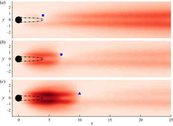
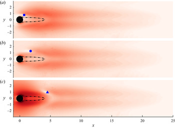
where  $\epsilon _{{OE}}^2$ denotes the mean kinetic energy of the estimation error throughout the domain (see Appendix D). Figure 7 uses the three sensor locations marked in figure 6(a), including the optimal location (
 $\bullet$, blue), one located upstream (
 $\blacksquare$, blue) and one located downstream (
 $\blacktriangle$, blue), to show the effect of the sensor position on
 $\epsilon _{{OE}}$.
Spatial distribution of the estimation error  $\epsilon _{{OE}}$ at
 ${\textit {Re}}=60$. Three different sensor locations shown in figure 6(a) are tested, which are marked by (a) (
 $\blacksquare$, blue); (b) (
 $\bullet$, blue) (optimal); (c) (
 $\blacktriangle$, blue). The optimal estimators are designed using the parameters
 $k=3$ and
 $\omega _n=9$. The dash–dotted line (–
 $\cdot$ –) indicates the boundary of the reverse-flow region and all plots share the same linear colour scale.

In all three cases, the smallest value of  $\epsilon _{{OE}}$ occurs at the sensor location. The most significant contributions to the estimation error are concentrated in two horizontal streaks which are approximately symmetric and located around
 $y\approx 0.7$. The reduction of
 $\epsilon _{{OE}}$ at the sensor location divides these two streaks into two regions: a near-wake area (between the cylinder and the sensor) and a far-wake area (downstream of the sensor). If the sensor is placed too far upstream, the upstream estimation error is naturally dampened but the downstream flow is not observable to the sensor and, thus, the estimation error develops in the large far-wake area. When the sensor moves downstream, the estimation error is strongly amplified in the near-wake area, as shown in figure 7(c). The optimal placement of the sensor should therefore balance minimising the estimation error that is amplified in the near-wake area against minimising that developing in the far-wake area, which agrees with the findings for a spatially developing one-dimensional flow (Oehler & Illingworth Reference Oehler and Illingworth2018).
4.1.2. Optimal sensor placement
We are interested in the optimal sensor locations to achieve the best estimation performance for different Reynolds numbers. Brute-force sampling is inefficient when searching for global optimal placements for different Reynolds numbers. Instead, we now employ a gradient minimisation method (e.g. Newton's method) together with sensible initial guesses chosen based on the observations of figure 6.
Coordinates of the optimal sensor location are plotted in figure 8(a,b) as a function of the Reynolds number. It can be seen that, as the Reynolds number increases, the optimal streamwise location  $x_{s-opt}$ moves downstream whereas the optimal transverse location
 $y_{s-opt}$ remains approximately constant (
 $0.73\pm 0.01$). This trend is consistent with the evolution of the reverse-flow region shown in figure 8(c), which also closely approximates the absolutely unstable (AU) region (Pier Reference Pier2002). The length of the AU region behind the circular cylinder increases with increasing Reynolds number, which pushes the optimal sensor location downstream. However, to avoid excessive time lag, the migration of the optimal sensor location downstream is much slower than the evolution of the AU region: the optimal sensor location moves only
 $1.8$ diameters downstream whereas the length of the AU region extends
 $3.8$ diameters further when the Reynolds number increases from
 $50$ to
 $110$. This is a result of the convection-driven nature of the system: at higher Reynolds numbers, the instability develops more rapidly while convecting downstream and, thus, there exists a larger effective phase lag in the measurements when the sensor is placed at a fixed distance downstream of the AU region. This is consistent with the findings of Oehler & Illingworth (Reference Oehler and Illingworth2018), where the optimal sensor locations found for the OE problem moved upstream to compensate for any artificial time lag that was imposed on the system.
Coordinates of the optimal sensor location (a)  $x_{s-opt}$ and (b)
 $y_{s-opt}$ as a function of the Reynolds number. (c) The profile of the reverse-flow region (the grey area) at different Reynolds numbers. (d) The OE performance as a function of the Reynolds number. Here
 $\gamma ^2{(k,\omega _n)}$ is the cost function for the estimator design (
 $k=3$,
 $\omega _n=9$), whereas
 ${\boldsymbol {J}}_{OE}$ represents the mean kinetic energy of the total estimation error evaluated from numerical simulations with random disturbances applied everywhere.

It is also interesting to note that, although the AU region extends further downstream with increasing Reynolds number, it barely changes in the transverse direction. As a result, the optimal transverse position remains almost constant over the Reynolds number range considered. Meanwhile, the cost function  $\gamma ^2{(k,\omega _n)}$ for the estimator design, which considers only the first
 $k$ resolvent modes over the frequency range
 $\omega \in [-\omega _n, \omega _n]$, increases logarithmically, as shown in figure 8(d). To evaluate the OE performance when random disturbances are applied everywhere, we simulate the closed-loop error system with the optimal sensor placement and the optimal estimator. The mean kinetic energy of the total estimation error
 $\boldsymbol {J}_{OE}$, as defined by (3.2), is plotted as a function of the Reynolds number in figure 8(d). Similarly, the estimation performance
 $\boldsymbol {J}_{OE}$ also increases logarithmically with increasing Reynolds number. The gap between
 $\gamma ^2{(k,\omega _n)}$ and
 $\boldsymbol {J}_{OE}$ represents the contribution from the ‘background’ or ‘free-stream’ modes that are excluded while designing the optimal estimator. We notice that this gap accounts for
 $91\,\%$ of the total estimation error at
 $Re=50$ but decreases to
 $75\,\%$ of the total at
 $Re=110$. This suggests that the cost function
 $\gamma ^2{(k,\omega _n)}$ better approximates the total estimation error
 $\boldsymbol {J}_{OE}$ at higher Reynolds numbers. Note that the solution of the optimisation problem (e.g. optimal estimator, optimal sensor placement) is determined by the gradient of the cost function (i.e. by setting the gradient equal to zero). Therefore, although there is a large gap between
 $\gamma ^2{(k,\omega _n)}$ and
 $\boldsymbol {J}_{OE}$, both of them give the same optimal location.
4.1.3. Effect of domain size
In the OE problem, we simply choose to optimally estimate the entire flow field, which is influenced by two different mechanisms: (i) the growth of flow perturbations due to the strong shear layer in the near-wake area of the base flow; (ii) the transportation of flow perturbations to the far-wake area due to the convective nature of the flow. Due to the lack of nonlinear energy transfer to higher frequencies, any flow perturbations will grow and be transported far downstream of the cylinder until they dissipate. However, this leads to two significant problems. First, in contrast to the optimal placements in other control problems, the optimal sensor location in the OE problem is sensitive to the streamwise extent of the computational domain. When the domain is extended in the streamwise direction, i.e. estimation extends further downstream, the optimal sensor location also moves downstream. This can be clearly seen in figure 9 where the optimal sensor location at  ${\textit {Re}}=110$ is plotted as a function of the streamwise extent of the domain. In particular, the streamwise coordinate
 $x_{s-opt}$ does not converge even when the domain extends to 100 diameters downstream of the cylinder. Second, the optimal sensor placement found for the OE problem is not optimal for feedback control. Intuitively, the upstream growth of flow perturbations should be the main concern for feedback control and the control of their convection downstream would not be effective at minimising flow perturbations. Indeed, we will see later that the optimal locations of either the actuator or the sensor found for feedback control are always upstream or near the edge of the reverse-flow region whereas the sensor in the OE problem is best placed far downstream. Together these observations indicate that the OE problem, although interesting, is not the most suitable method for placing sensors for feedback control. Therefore, effective estimation of the flow field does not guarantee effective control performance and vice versa. Similar conclusions have been drawn while investigating the sensor placement problem for a one-dimensional flow (Oehler & Illingworth Reference Oehler and Illingworth2018) and for the cylinder flow using deep reinforcement learning (Paris, Beneddine & Dandois Reference Paris, Beneddine and Dandois2021). Note that the OE problem considered in this study is merely a part of the whole optimal feedback control problem. Although the optimal sensor placement found for the OE problem varies with the domain size, the computational domain described in figure 1 results in converged optimal placements for the other control problems considered.
Coordinates of the optimal sensor location (a)  $x_{s-opt}$ and (b)
 $y_{s-opt}$ at
 ${\textit {Re}}$=110 when the domain is extended in the streamwise direction. Here
 $X_{outlet}$ is the position of the outlet boundary.

4.2. Full-state information control problem
4.2.1. Brute-force sampling
We now turn our attention to the FIC problem and the corresponding optimal actuator placement problem. Analogous to the OE problem, a brute-force sampling approach for the FIC problem is performed at  ${\textit {Re}}=60$ and
 ${\textit {Re}}=110$ with the same parameters (
 $k=3$,
 $\omega _n=9$) as those used in the OE problem. The corresponding cost function
 $\gamma ^2{(k,\omega _n)}$ is mapped as a function of the actuator location (
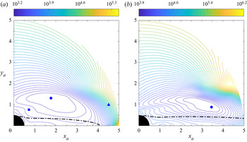
 $x_{a},\ y_{a}$) in figure 10, where the dash–dotted line indicates the region of reverse flow.
Contours of the cost function  $\gamma ^2{(k,\omega _n)}$ in the FIC problem and the optimal actuator locations (
 $\bullet$, blue) at (a)
 ${\textit {Re}}=60$ and (b)
 ${\textit {Re}}=110$. The square (
 $\blacksquare$, blue) and triangle (
 $\blacktriangle$, blue) correspond to the actuator locations considered in figure 11. Controllers are designed using the parameters
 $k=3$ and
 $\omega _n=9$. The dash–dotted line (–
 $\cdot$ –) indicates the boundary of the reverse-flow region.

We first note that the global optimal actuator ( $\bullet$, blue) is located at approximately
 $(x_a, y_a)=(1.77,\ 1.31)$ for
 ${\textit {Re}}=60$ and at
 $(x_a, y_a)=(3.46,\ 0.88)$ for
 ${\textit {Re}}=110$. Similar to the OE problem, only one minimum appears in the sampled area at each Reynolds number, which is therefore the global optimum. The performance of an full-state information controller with the actuator placed outside the sampled area is far worse than that with an actuator placed inside the sampled area. It is reasonable to suppose that the optimal actuator locations for the Reynolds numbers considered in this study will always be in the near-wake area and outside the reverse-flow region. As can be seen from figure 10, we expect that, with increasing Reynolds number, the optimal actuator placement will move not only downstream but also closer to the reverse-flow region. These observations provide reasonable initial guesses for the optimal placement problem at different Reynolds numbers and a traditional gradient minimisation method (e.g. Newton's method) is sufficient to solve this non-convex problem. Another significant feature observed from the topography of the cost function in figure 10 is that a ‘cliff’ appears slightly downstream of the optimal actuator position at each Reynolds number, where the cost function increases rapidly. This occurs because the shift in the actuator location across the ‘cliff’ causes a right-half-plane (RHP) zero to appear near the unstable pole in the
 ${\boldsymbol {q}}$-to-
 ${\boldsymbol {y}}$ transfer function. This imposes a severe limitation on the controller's ability to reject disturbances (see Skogestad & Postlethwaite (Reference Skogestad and Postlethwaite2007) and the discussion of figure 11).
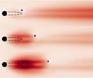
Spatial distribution of the receptivity to disturbance  $\epsilon _{{FIC}}$ at
 ${\textit {Re}}=60$. Three different actuator locations shown in figure 10(a) are tested, which are marked by (a) (
 $\blacksquare$, blue); (b) (
 $\bullet$, blue) (optimal); (c) (
 $\blacktriangle$, blue). The optimal controllers are designed with
 $k=3$ and
 $\omega _n=9$. The dash–dotted line (–
 $\cdot$ –) indicates the boundary of the reverse-flow region and all plots share the same logarithmic colour scale.

In order to clearly show the controller's disturbance rejection performance for different actuator placements, we plot the root-mean-square value  $\epsilon _{{FIC}}$ in figure 11, which is defined similarly to (4.1) (see Appendix D). Analogous to the OE problem, we only consider the first
 $k$ resolvent modes within the frequency range
 $\omega \in [-\omega _n,\omega _n]$ to make the computation tractable. Here, the term
 $\epsilon _{{FIC}}^2$ indicates the contribution of each and every disturbance to the mean kinetic energy of flow perturbations under closed-loop control. In other words, it shows the spatial distribution of the receptivity of the closed-loop system to disturbances. The darker regions in figure 11 have higher receptivity, which implies that the flow is sensitive to disturbances (poorer disturbance rejection ability) under the control of the actuator.
In order to show the effect of actuator position on  $\epsilon _{{FIC}}$, figure 11 uses the three actuator locations marked in figure 10(a): the optimal location (
 $\bullet$, blue), one located upstream (
 $\blacksquare$, blue) and one located downstream (
 $\blacktriangle$, blue). The same logarithmic colour scale is used for all three contour plots. In each case, the minimum value of
 $\epsilon _{{FIC}}$ occurs at the location of the actuator, which is where the disturbance's influence can be directly eliminated. We also see that, for all three plots, there is a small white area upstream of the actuator rather than downstream of it. Therefore, the actuator is better able to reject the influences of disturbances that occur immediately upstream of the actuator than those that occur immediately downstream. Another significant observation from these contour plots is that the spatial distribution of
 $\epsilon _{{FIC}}$ can also be divided into two regions: the first is the near-wake area (upstream of the actuator) and the second is the far-wake area (downstream of the actuator). If the actuator is placed too close to the cylinder, it successfully rejects upstream disturbances but fails to suppress disturbances in the large far-wake area, as shown by figure 11(a). But if the actuator is moved to the far-wake area, the situation becomes much worse, as shown in figure 11(c), where the influence of upstream disturbances is much greater than for the other two cases. This occurs because the actuator is located inside the ‘cliff’ region presented in figure 10(a). The optimal actuator position should therefore allow the actuator to handle the effect of disturbances from both the near-wake area and the far-wake area, which is consistent with previous results for the one-dimensional Ginzburg–Landau equation (Oehler & Illingworth Reference Oehler and Illingworth2018).
4.2.2. Optimal actuator placement
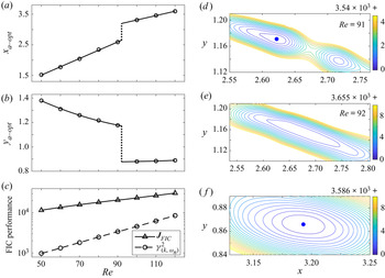
To locate the optimal actuator positions at different Reynolds numbers, we employ the same gradient minimisation method as that used in the OE problem with sensible initial guesses chosen based on the results of figure 10. The corresponding optimal placements and their control performances are summarised in figure 12. We see that the optimal actuator position ( $x_{a-opt}$,
 $y_{a-opt}$) moves downstream and closer to the recirculation zone as the Reynolds number increases. This trend is the opposite of that observed for a spatially developing one-dimensional flow where the optimal actuator placement moves upstream with increasing instability (Oehler & Illingworth Reference Oehler and Illingworth2018). This occurs because the AU region, as shown in figure 8(c), extends only further downstream when the instability increases, whereas it also expands upstream in the one-dimensional Ginzburg–Landau equation. The cost function
 $\gamma ^2{(k,\omega _n)}$ for the full-state information controller design and the optimal control performance
 ${\boldsymbol {J}}_{FIC}$ from numerical simulations are plotted as a function of the Reynolds number in figure 12(c). Both quantities increase logarithmically with increasing Reynolds number and the gap between them represents the contribution from the ‘background’ or ‘free-stream’ modes that are not important for the optimal controller design (see Appendix C).
(a–c) Coordinates of the optimal actuator location (a)  $x_{a-opt}$ and (b)
 $y_{a-opt}$ as a function of the Reynolds number. (c) The optimal FIC control performance as a function of the Reynolds number. Here
 $\gamma ^2{(k,\omega _n)}$ is the cost function for the controller design (
 $k=3$,
 $\omega _n=9$), whereas
 ${\boldsymbol {J}}_\textrm {FIC}$ is the mean kinetic energy of flow perturbations from numerical simulations where random disturbances are applied everywhere. A discontinuity in the optimal actuator location (
 $\cdot \cdot \cdot \cdot \cdot$) occurs around
 ${\textit {Re}}\approx 92$. (d–f) Contours of the cost function
 $\gamma ^2{(k,\omega _n)}$ for divisions of the minima at (d)
 ${\textit {Re}}=91$ and (e,f)
 ${\textit {Re}}=92$ where the discontinuity occurs. The global optimal actuator positions are marked by a blue dot (
 $\bullet$, blue).

Another interesting feature observed is that there exists a discontinuity in the optimal actuator location around  ${\textit {Re}}\approx 92$, as indicated by the dotted line in figure 12(a,b). To clearly show why it occurs, we plot contours of the cost function near the optimal positions at
 ${\textit {Re}}=91$ and
 ${\textit {Re}}=92$ in figure 12(d,e). First of all, we identify that one global minimum dominates the near-wake area for
 ${\textit {Re}}\leq 90$ but that it splits into two local minima at
 ${\textit {Re}}=91$, as shown in 12(d). The blue dot (
 $\bullet$, blue) marks the global optimal actuator location which still follows the trend of the optimal actuator placement before the discontinuity occurs. Second, these local minima move relatively far from each other at
 ${\textit {Re}}=92$ and, thus, we show them separately using two panels in figure 12(e,f). In this case, the global optimum, as marked by the blue dot (
 $\bullet$, blue), switches to the one with the lower transverse position which is far downstream and follows this path at higher Reynolds numbers. Note that at a slightly higher Reynolds number, e.g.
 ${\textit {Re}}=93$, the local minimum shown in (e) disappears and only the downstream minimum in (f) remains. Third, even though the optimal position changes rapidly near
 ${\textit {Re}}=92$, any corresponding discontinuity in the control performance is barely observable in figure 12(c). In both cases, the difference in the control performance between these two local minima is small (<2 %). A similar discontinuity has also been observed in the spacing and the frequency of vortex shedding around
 ${\textit {Re}}\approx 90$ which reveals a small transition of the wake's instability (Tritton Reference Tritton1959; Lienhard Reference Lienhard1966).
4.3. Collocated input–output control problem
4.3.1. Brute-force sampling
We now look at the CIOC problem depicted in figure 3(c), where a single collocated actuator–sensor pair is available for measurement and control. The results of the OE and FIC problems have shown success in solving optimal placement problems and help us to understand the challenges of sensor and actuator placement. In this case, a single actuator and a single sensor are placed together such that a localised feedback loop is formed. Brute-force sampling for the CIOC problem is performed at  ${\textit {Re}} = 60$ and
 ${\textit {Re}} = 110$ with the parameters
 $k=3$ and
 $\omega _n=9$. The corresponding cost function
 $\gamma ^2{(k,\omega _n)}$ is mapped as a function of the location of the actuator–sensor pair (
 $x_c$,
 $y_c$) in figure 13, where the dash–dotted line indicates the reverse-flow region.
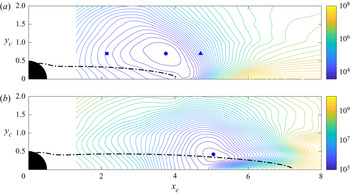
Contours of the cost function  $\gamma ^2{(k,\omega _n)}$ in the CIOC problem and the optimal locations of the collocated actuator–sensor pair (
 $\bullet$, blue) at (a)
 ${\textit {Re}}=60$ and (b)
 ${\textit {Re}}=110$. Feedback controllers are designed using the parameters
 $k=3$ and
 $\omega _n=9$. The dash–dotted line (–
 $\cdot$ –) indicates the boundary of the reverse-flow region.

As can be seen from figure 13, the optimal position for the collocated actuator–sensor pair occurs at approximately  $({x_c,\ y_c})=(3.75,\ 0.70)$ at
 ${\textit {Re}}=60$ and at approximately (
 ${x_c,\ y_c})=(5.05,\ 0.42)$ at
 ${\textit {Re}}=110$. Analogous to the OE and FIC problems, only a single local minimum appears in the sampled area at each Reynolds number, which is therefore the global optimum for the optimal placement problem of a collocated actuator–sensor pair. With increasing Reynolds number, this optimum moves downstream and closer to the edge of the reverse-flow region. Another significant observation from figure 13 is that a ‘cliff’ appears near
 $x_c\approx 5$ and along the centreline at both Reynolds numbers, where the cost function increases rapidly. This is due to the actuator being placed at a position with small receptivity to momentum forcing and a RHP zero occurs near the unstable pole in the
 ${\boldsymbol {q}}$-to-
 ${\boldsymbol {y}}$ transfer function, which imposes a severe limitation on the actuator's ability to control.
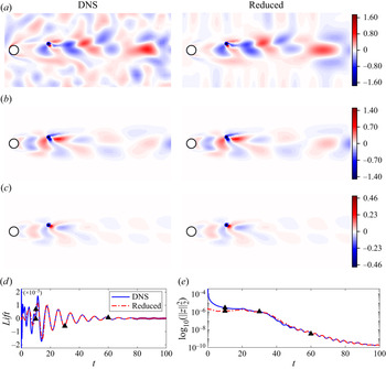
To more clearly show the control performance, we implement the optimal feedback control using an optimally placed collocated actuator–sensor pair in the fully nonlinear Navier–Stokes equations at  ${\textit {Re}}=60$. Here, direct numerical simulations (DNS) are performed using the IPCS (incremental pressure correction scheme) method which has been extensively tested on the computing platform FEniCS (Logg et al. Reference Logg, Mardal and Wells2012). We compare numerical simulations of two cases: (i) the actual nonlinear flow (i.e. DNS); (ii) the linear reduced model used for control design (i.e. by using reduced POD bases
 $\tilde {\boldsymbol {F}}_m$ and
 $\tilde {\boldsymbol {U}}_m$). The initial conditions for both cases are the impulse responses of an input that is modelled as uncorrelated random disturbances applied over the entire velocity field, with a magnitude of
 $1\times 10^{-4}$. The resulting control performance for each case is shown in figure 14.
Comparisons of feedback control results from DNS (—–, blue) and the linear reduced model (–  $\cdot$ –, red) at
 $Re=60$ using the optimal collocated set-up (
 $\bullet$). (a–c) Vorticity contours from DNS and the reduced linear model at
 $t=10, 30, 60$ (
 $\blacktriangle$, black). (d,e) Time evolution of the lift acting on the circular cylinder and the total perturbation energy
 $\|{\boldsymbol {z}}\|_2^2$ in log scale. The colour ranges of contour plots are scaled by
 $10^{-3}$.

Figure 14(a–c) shows comparisons of the instantaneous perturbation vorticity fields from the actual nonlinear flow and the linear reduced model at three different time steps:  $t=10, 30, 60$. At
 $t=10$ we observe good agreement between the nonlinear flow and the linear reduced model in the near weak. We do, however, observe some differences in the free stream. In particular, we observe strong responses in the free-stream area of the nonlinear flow field whereas the free-stream perturbation vorticity is almost zero in the linear reduced model. Although random disturbances are applied over the entire domain, the linear reduced model only considers dominant resolvent modes and excludes the contribution from ‘background’ modes that are concentrated in the free stream (see figure 4). Second, the perturbation vorticity fields at
 $t=30$ are almost identical for the nonlinear flow and the linear reduced model with only slight differences in the far downstream. It indicates that a small number of dominant modes are sufficient to characterise linear flow physics since the truncated ‘background’ modes are irrelevant to flow control and are soon damped out. This can be more clearly seen in figure 14(c) where the perturbation vorticity fields of both cases appear identical even in the far downstream and the linear reduced model accurately reconstructs the nonlinear flow.
Figure 14(d,e) further shows the time evolution of the lift acting on the circular cylinder and the total perturbation energy. Here, blue solid lines (—–, blue) and red dot–dashed lines (–  $\cdot$ –, red) denote physical quantities from the nonlinear flow and the linear reduced model, respectively. The two simulations match when
 $t>20$ and their differences at the early stage (i.e.
 $t<20$) represent the contribution from ‘background’ modes that are truncated in the linear reduced model. Note that neither lift nor perturbation energy comes from the sensor measurement and the control design method considers the reconstruction of the whole flow field instead of recovering merely the sensor information. Although only the first three resolvent modes within the frequency range
 $\omega \in [-9, 9]$ rad s
 $^{-1}$ are considered, the linear reduced model accurately reproduces the true nonlinear flow.
4.3.2. Optimal actuator–sensor placement
The optimal positions of the collocated actuator–sensor pair are found using the same gradient minimisation method described in § 4.1 with sensible initial guesses at different Reynolds numbers. The results are displayed in figure 15(a,b). The optimal location moves downstream with increasing Reynolds number, which is consistent with the trends observed for both the OE and FIC problems. Meanwhile, the optimal transverse position  $y_{c-opt}$, as shown in figure 15(b), decreases and eventually converges to a constant position at higher Reynolds numbers. Both the cost function
 $\gamma ^2{(k,\omega _n)}$ and the optimal control performance
 ${\boldsymbol {J}}_{CIOC}$ are summarised in figure 15(c). In particular, they rise approximately logarithmically with increasing Reynolds number and the gap between them becomes increasingly negligible at higher Reynolds numbers. This is because the contributions from the neglected ‘background’ or ‘free-stream’ modes remain approximately constant regardless of any control, as concluded from figure 18. As a result, they account for a smaller proportion of the total kinetic energy of flow perturbations at higher Reynolds numbers. The comparisons of optimal placements and their performances found for the OE, FIC and CIOC problems will be presented in § 4.4.1.
Coordinates of the optimal actuator–sensor location (a)  $x_{c-opt}$ and (b)
 $y_{c-opt}$ as a function of the Reynolds number. (c) The optimal feedback control performance as a function of the Reynolds number. Here
 $\gamma ^2{(k,\omega _n)}$ is the cost function for the feedback controller design (
 $k=3,\ \omega _n=9$), whereas
 ${\boldsymbol {J}}_{CIOC}$ is the mean kinetic energy of flow perturbations evaluated from numerical simulations with random disturbances applied everywhere.

4.4. Trade-offs for optimal placement
We now compare the main results of the OE, FIC and CIOC problems, and discuss the implications for effective input–output (feedback) control. Any fundamental trade-offs and key factors that limit effective estimation and control will be explored. In particular, the coupling effect between the sensor and the actuator (i.e. the time lag) is important due to the convective nature of the flow, and we will highlight the decisive influence of excessive time delay on the sensor and actuator placements. To better demonstrate this, we compare three different IOC set-ups: (i) using an optimally placed collocated actuator–sensor pair (i.e. CIOC); (ii) using optimal sensor and actuator placements found for the OE and FIC problems separately (i.e. IOC $_{{sep}}$); (iii) using an optimally placed actuator and an optimally placed sensor (i.e. IOC
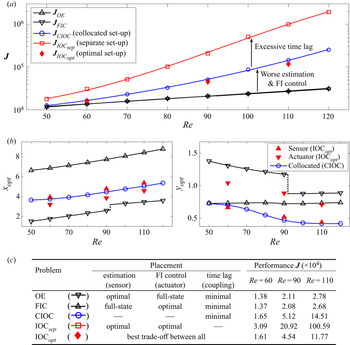
 $_{{opt}}$). Sensor and actuator placements and their performances for each problem are plotted as a function of the Reynolds number in figure 16(a,b). Details of the problem set-ups and their optimal performances achieved are then summarised in the table beneath.
Comparisons of the optimal performances and the optimal placements between different problem set-ups. (a) The optimal performance  ${\boldsymbol {J}}$ as a function of the Reynolds number in the OE (lined downtriangle, black), FIC (lined triangle, black), CIOC (collocated set-up, lined circle, blue), IOC
 $_{{sep}}$ (separate set-up, lined square, red) and IOC
 $_{{opt}}$ (optimal set-up,
 $\diamond$, red) problems. (b) Coordinates of optimal placements as a function of the Reynolds number. (c) A summary of set-ups for all problems and their optimal performances at
 ${\textit {Re}}=60, 90, 110$.

4.4.1. Comparisons of OE, FIC and CIOC problems
We first consider the OE problem (represented by lined triangle, black) and the FIC problem (represented by lined downtriangle, black), in which the sensor and actuator are each placed to achieve the best estimation and FIC performance possible, respectively. From figure 16(a) we first note that the optimal OE performance  ${\boldsymbol {J}}_{OE}$ (lined triangle, black) and the optimal FIC performance
 ${\boldsymbol {J}}_{FIC}$ (lined downtriangle, black) are almost identical for each Reynolds number considered. As aforementioned, the OE problem can be recast as a unity feedback control problem for the estimation error with perfect actuation, and the optimal sensor placement strikes a balance between measuring the flow upstream and measuring the flow downstream to provide the best observation of the entire flow. Similarly, the FIC problem provides perfect measurements of the entire flow field, and the optimal actuator placement achieves the best FIC performance by striking a balance between attenuating flow perturbations upstream and attenuating flow perturbations downstream. The differences between the OE and FIC problems are summarised in figure 16(c), and the similarities between their optimal performances implies that neither the sensor placement nor the actuator placement is the key factor that limits control performance. It is also interesting to note that there exists a large spatial separation between the optimal sensor placements for the OE problem (lined triangle, black) and the optimal actuator placements for the FIC problem (lined downtriangle, black), as shown in figure 16(b). This is mainly caused by the convective non-normality of the cylinder flow, which leads to upstream-leaning forcing modes and downstream-leaning response modes.
We further consider the CIOC problem (represented by lined circle, blue) in which the minimal possible time lag between actuation and sensing is achieved. In this scenario, the optimal placement of the collocated actuator–sensor pair ensures the best trade-off between maintaining good estimation performance and maintaining good FIC performance. We can see that  ${\boldsymbol {J}}_{CIOC}$ (lined circle, blue) is significantly larger than either
 ${\boldsymbol {J}}_{OE}$ or
 ${\boldsymbol {J}}_{FIC}$, particularly at higher Reynolds numbers, as shown in figure 16(a). This performance deterioration is mainly caused by two factors: (i) the perfect spatially distributed actuation (in the OE problem) and the perfect spatially distributed sensing (in the FIC problem) degenerate to a single-point actuator and a single-point sensor in the CIOC problem; (ii) neither the sensor nor the actuator is optimally placed, both of which contribute to poorer estimation and control of the entire flow than for the OE and FIC problems separately. As shown in figure 16(b), the optimal placement of the collocated actuator–sensor pair (lined circle, blue) is located between the optimal placements found for the OE and FIC problems, which is expected behaviour.
4.4.2. Input–output control using optimal placements of OE and FIC
The input–output controller that results from the independently designed optimal estimator and the independently designed optimal full-state information controller is still optimal, as stated by the separation principle of estimation and control. However, the optimal placements found for the OE and FIC problems are not necessarily optimal for the IOC problem. That is, the optimal placement problem does not satisfy the separation principle. To better demonstrate this, we now consider the IOC problem that uses a set-up where a single sensor is placed at the optimal location found for the OE problem to provide the best estimation of the entire flow and a single actuator is placed at the optimal location found for the FIC problem to provide the best FIC of the entire flow. This set-up utilises optimal sensor and actuator locations that were found independently for the OE and FIC problems, and is thus denoted by IOC $_{{sep}}$ (lined square, red) in figure 16. Although the best estimation performance and the best FIC performance are each ensured, the corresponding feedback control (IOC) performance exhibits a more severe deterioration when compared with the CIOC problem, as shown in figure 16(a). In particular, the cost function
 ${\boldsymbol {J}}_{{IOC}_{{sep}}}$ is 87 % higher than
 ${\boldsymbol {J}}_{CIOC}$ at
 ${\textit {Re}}=60$ and it is 593 % higher at
 ${\textit {Re}}=110$, as listed by the table in figure 16(c).
As discussed in § 4.1.3, one possible reason for the performance deterioration is that the sensor in the OE problem and the sensor in the feedback control problem are required to measure different information to achieve their respective best performance. Although the optimal sensor placement found for the OE problem provides the best estimation of the entire flow field (e.g. both instability activities and transportation of flow perturbations), it fails to optimally estimate the information that would be the most beneficial for feedback control. Another significant reason is the excessive time lag between the sensor and the actuator, which has a much stronger influence for the IOC problem. This is caused by the convective nature of the cylinder flow. The sensor and actuator placements that are most effective for feedback control should therefore give priority to reducing the time lag between actuation and sensing.
4.4.3. Optimal IOC and the effect of time delay
The effect of time lag can be more clearly shown by considering the optimal set-up for the IOC problem, in which an optimally placed sensor and an optimally placed actuator are used to achieve the best IOC performance. It is computationally expensive to find such placements for a two-dimensional flow since the optimisation problem is four dimensional (locating the optimal sensor and optimal actuator placements simultaneously). Therefore, we only present results for  ${\textit {Re}}=60,\ {\textit {Re}}=90\ \text {and}\ {\textit {Re}}=110$. These results are represented by IOC
 $_{{opt}}$ (
 $\diamond$, red) in figure 16. As can be seen from figure 16(a), the control performance
 ${\boldsymbol {J}}_{{IOC}_{{opt}}}$ is only slightly smaller than
 ${\boldsymbol {J}}_{CIOC}$ (lined circle, blue). It is approximately 2.5 % lower at
 ${\textit {Re}}=60$ and 19 % lower at
 ${\textit {Re}} =110$, as listed in figure 16(c).
We also note that the optimal sensor and actuator placements in the IOC $_{{opt}}$ problem (lined triangle, red/lined downtriangle, red) are close to those found for the CIOC problem (lined circle, blue), as shown in figure 16(b). The optimal placement of a collocated actuator–sensor pair therefore seems to provide a good approximation of the optimal feedback control set-up for the cylinder flow. In particular, the optimal sensor locations (lined triangle, red) for feedback control show good agreement with the optimally placed collocated actuator–sensor pair (lined circle, blue) in the CIOC problem at both Reynolds numbers. As for the optimal actuator positions (lined downtriangle, red), their streamwise coordinates (i.e.
 $x_{opt}$) are slightly upstream of those found for the CIOC problem (lined circle, blue) whereas their transverse coordinates lie between those found for the FIC problem and those found for the CIOC problem.
This observation is not consistent with the intuition put forward by many previous studies that maintaining accurate flow estimation and maintaining effective FIC are essential for efficient feedback control (Cohen, Siegel & McLaughlin Reference Cohen, Siegel and McLaughlin2006; Seidel et al. Reference Seidel, Siegel, Fagley, Cohen and McLaughlin2009). Specifically, the best sensor location for feedback control should be close to that found for the OE problem and the best actuator location for feedback control should be close to that found for the FIC problem. This is true in some previous studies for simpler spatially developing flow models, e.g. for the one-dimensional Ginzburg–Landau equation (Oehler & Illingworth Reference Oehler and Illingworth2018). However, the current study reveals that minimising the time-lag effect is of higher priority for feedback control of the two-dimensional cylinder flow. One possible explanation for the consistency between the optimal placements found for the CIOC problem and those found for the IOC problem is the convective nature of the cylinder flow which leads to a strong time-lag effect between the separately placed sensor and actuator. Indeed, by introducing an artificial time delay into the one-dimensional Ginzburg–Landau equation, the optimal sensor and actuator locations in the feedback control problem move closer to each other and lead to similar results as those shown in the current study (Oehler & Illingworth Reference Oehler and Illingworth2018). This supports the observation that the time lag is indeed the major factor that determines the optimal placement of control devices in the two-dimensional cylinder flow.
5. Conclusions
We have considered optimal estimation and control of linear perturbations in the flow past a two-dimensional circular cylinder over a range of Reynolds numbers. In particular, we focused on the optimal placement of a single sensor and a single actuator to better understand the limitations of effective feedback control. Although the corresponding optimal placement problems are non-convex, brute-force sampling results for each problem revealed a unique local optimal position in the wake area which represents the global optimum. A simple gradient minimisation method was then sufficient to locate the optimal positions at each Reynolds number. It was shown that the optimal sensor and actuator locations move downstream as the Reynolds number increases, and their trajectories presented conflicting trade-offs. In the OE problem, the sensor should be placed where it achieves the best compromise between measuring the flow upstream and measuring the flow downstream to provide optimal observations of the entire flow. In the FIC problem, the optimal actuator placement should strike a balance between controlling the near-wake area (which displays receptivity to disturbances) and controlling the far-wake area where the remaining disturbances can potentially be amplified.
For the input–output (feedback) control problem in which the sensor and actuator placements are coupled, the effect of excessive time lag results in optimal sensor and actuator locations that are close to each other in the streamwise direction. In particular, the optimal placement of a collocated actuator–sensor pair was shown to be a good approximation for the actual optimal placements for feedback control. For fluid flows that are dominated by convection, e.g. the cylinder flow, reducing the time lag between actuation and sensing appears to be crucial for achieving good feedback control performance.
Funding
This research received no specific grant from any funding agency, commercial or not-for-profit sectors.
Declaration of interests
The authors report no conflict of interest.
Appendix A. The systems for estimation and control
Table 1 lists the system states, inputs, outputs and Riccati equations for the OE, FIC and IOC problems. Note that the state-space model of the IOC problem is assembled from two subsystems of the OE and FIC problems. The corresponding state matrices are  $\tilde {\boldsymbol {E}}=\boldsymbol {diag}[\boldsymbol {E},\boldsymbol {E}]$ and
 $\tilde {\boldsymbol {A}}=\boldsymbol {diag}[\boldsymbol {A},\boldsymbol {A}]$, where
 $\boldsymbol {diag}[\cdot ]$ indicates a block-diagonal matrix built from the provided matrices. Therefore, all three problems can be cast into the same general form (A1) (Kim & Bewley Reference Kim and Bewley2007; Skogestad & Postlethwaite Reference Skogestad and Postlethwaite2007; Chen & Rowley Reference Chen and Rowley2011),
 \begin{equation} \begin{bmatrix} \tilde{\boldsymbol{E}}\dot{{\boldsymbol{x}}}\\ {\boldsymbol{y}}\\ {\boldsymbol{z}} \end{bmatrix}= \begin{bmatrix} \tilde{\boldsymbol{A}} & \boldsymbol{B}_1 & \boldsymbol{B}_2 & \boldsymbol{0}\\ \boldsymbol{C}_1 & \boldsymbol{0} & \boldsymbol{0} & \boldsymbol{V}^{1/2}\\ \boldsymbol{C}_2 & \boldsymbol{R}^{1/2} & \boldsymbol{0} & \boldsymbol{0} \end{bmatrix} \begin{bmatrix} {\boldsymbol{x}}\\ {\boldsymbol{q}}\\ {\boldsymbol{d}}\\ {\boldsymbol{n}} \end{bmatrix}. \end{equation}
In particular, the optimal estimator gain  $\boldsymbol {K}_f$ and the FIC gain
 $\boldsymbol {K}_r$ are formed from the solutions of the algebraic Riccati equations associated with the OE and FIC problems (i.e.
 $\boldsymbol {X},\ \boldsymbol {Y}$). The covariance matrices for the OE and FIC problems are
 $\boldsymbol {W}_1=\boldsymbol {B}_d\boldsymbol {B}_d^T$ and
 $\boldsymbol {W}_2=\boldsymbol {C}_z^T\boldsymbol {C}_z$, respectively. In this case,
 $\boldsymbol {B}_d$ and
 $\boldsymbol {C}_z$ are the low-rank input and output matrices (see § 3.3) to overcome the difficulty of solving Riccati equations with full-state inputs and full-state outputs. The analytical expression for the
 $\mathcal {H}_2$ norm for the closed-loop system
 $\boldsymbol {G}(s)$ can thus be written as
 \begin{align} \lVert{\boldsymbol{G}(s)}\rVert^2_2&=\underbrace{\textrm{tr}(\boldsymbol{C}_z\boldsymbol{X}\boldsymbol{C}_z^*)}_{OE}+
\underbrace{\textrm{tr}(\boldsymbol{V}^{{-}1}\boldsymbol{C}_y\boldsymbol{X}\boldsymbol{Y}\boldsymbol{X}
\boldsymbol{C}_y^*)}_{Cross\hbox{-}contribution} \nonumber\\
&=\underbrace{\textrm{tr}(\boldsymbol{B}_d\boldsymbol{Y}\boldsymbol{B}_d^*)}_{FIC}+
\underbrace{tr(\boldsymbol{R}^{{-}1}\boldsymbol{B}_q\boldsymbol{Y}\boldsymbol{X}
\boldsymbol{Y}\boldsymbol{B}_q^*)}_{Cross\hbox{-}contribution}
\end{align}
which consists of two terms: (i) a contribution from either the OE or FIC problem; (ii) a cross-contribution from the coupling effect between sensors and actuators in the IOC problem. Note that the latter term illustrates the failure of the separation principle for the coupled actuator–sensor placement problems from a mathematical point of view.
A summary of system states, matrices and Riccati equations for the OE, FIC and IOC problems.

Appendix B. Resolvent-based design method
This section presents detailed steps and results for designing the optimal estimator at  ${\textit {Re}}=90$, as summarised in figure 17. The optimal full-state information controller can be designed in an analogous manner. Note that resolvent analysis is central to this design method, which is able to predict dominant coherent structures even for higher Reynolds numbers (Toedtli, Luhar & McKeon Reference Toedtli, Luhar and McKeon2019; Ribeiro, Yeh & Taira Reference Ribeiro, Yeh and Taira2020). Therefore, the method is still potentially applicable when the flow becomes three dimensional and transitions to turbulent flow. The method is illustrated in the following three stages.
(i) Initialising. The resolvent operator
$\mathcal {H}(\kern0.06em j\omega )$ is first constructed from the frequency-domain Navier–Stokes equations linearised about the base flow, which is subsequently decomposed into the input and output matrices $\hat {\boldsymbol {F}}$ and $\hat {\boldsymbol {U}}$ each consisting of orthonormal modes ranked by their energy gains $\sigma _i$ in the diagonal matrix $\boldsymbol {\varSigma }$. The decomposition is performed at each sampling frequency within a specified range (e.g. $\omega _i\in [-\omega _n,\ \omega _n]$) and we consider a truncated input matrix $\hat {\boldsymbol {F}}_k$ (with only the first $k$ dominant input modes $\hat {{\boldsymbol {f}}}_i$ ) for optimal estimator design. The grey area of the line chart in the resolvent analysis panel represents the integrated energy gains (i.e. the cost function $\gamma ^2(k,\omega _n)$) that need to be minimised.(ii) Solving. The optimal estimator can be computed by solving the large-scale Riccati equation associated with the OE problem. We utilise a sparse Riccati solver (Saak et al. Reference Saak, Köhler and Benner2019) which can handle high-dimensional system matrices (i.e.
$\boldsymbol {A},\ \boldsymbol {E}\in \mathbb {R}^{N\times N}$) but the number of inputs (i.e. the rank of $\boldsymbol {B}_d$) is limited to be small. Here, $N$ denotes the dimensionality of the flow system. The matrix $\boldsymbol {B}_d$ represents statistical properties of disturbances, which are modelled as uncorrelated zero-mean Gaussian white noise and are injected over the entire velocity field. Thus, $\boldsymbol {B}_d\in \mathbb {R}^{N\times N}$ is a full-rank matrix and a low-rank approximation is required to solve the Riccati equation. In this study, the low-rank approximation $\tilde {\boldsymbol {F}}_m\in \mathbb {R}^{N\times m}$ is constructed from the most responsive resolvent input modes $\hat {\boldsymbol {F}}_k$ combined with POD analysis. Instead of the full-state random disturbances, we consider reduced random disturbances which disturb the system through random combinations of the dominant POD modes $\tilde {{\boldsymbol {f}}}_i$. The Riccati equation can then be solved by setting $\boldsymbol {B}_d\approx \tilde {\boldsymbol {F}}_m$. We update the resolvent operator of the closed-loop estimation error system by including the resulting estimator $\boldsymbol {K}_f$. As can be seen from the line chart in the resolvent analysis panel, the grey area is much smaller than that in the previous stage.(iii) Iterating. An iterative strategy is employed to further improve the estimation performance. In particular, we update the low-rank input space
$\tilde {\boldsymbol {F}}_m$ by including the new resolvent input modes (i.e. $\hat {\boldsymbol {F}}_k$) and the previous POD modes $\tilde {\boldsymbol {F}}_m$ in the POD analysis. As can be seen from the grey area of the line chart, the resulting estimator shows a better performance at higher frequencies, further minimising the cost function $\gamma ^2(k,\omega _n)$. We monitor the relative change of the estimation performance at each iteration until it reaches a stopping criterion.


Flow chart of optimal estimator design at  $Re=90$. (a) Initialising: construct resolvent operator
 $\mathcal {H}(\kern0.06em j\omega )$ of the open-loop system and perform resolvent analysis at each frequency
 $\omega _i$. (b) Solving: construct low-rank input space
 $\tilde {\boldsymbol {F}}_m$ using the resolvent input modes
 $\widehat {\boldsymbol {f}_i}$ combined with POD analysis and solve the Riccati equation. (c) Iterating: update the low-rank input space
 $\tilde {\boldsymbol {F}}_m$ by including new resolvent input modes in
 $\hat {\boldsymbol {F}}_k$ and solve the Riccati equation (Jin et al. Reference Jin, Illingworth and Sandberg2021).

Appendix C. Convergence analysis
This section presents the convergence analysis for the optimal performance and the optimal placement concerning the frequency range  $\omega _n$ and the number of resolvent modes
 $k$. The main results are summarised in table 2, where the OE problem is solved at
 ${\textit {Re}}=90$ for different choices of
 $\omega _n$ and
 $k$. Note that the cost function
 $\gamma ^2{(k,\omega _n)}$ is computed from the integration of the first
 $k$ energy gains (
 $\sigma _i^2$) of the closed-loop system across the frequency range
 $\omega \in [-\omega _n,\ \omega _n]$ (i.e. (3.4)), whereas the estimation performance
 ${\boldsymbol {J}}_{OE}$ is evaluated directly from numerical simulations when disturbances are applied everywhere in the domain (i.e. (3.2)). Any difference between them is accounted for by the less energetic modes that are neglected during the design of the optimal estimator.
The rank of the reduced disturbance  $m$, optimal sensor location of the OE problem (
 $x_{s-opt}$,
 $y_{s-opt}$), the cost function
 $\gamma ^2{(k,\omega _n)}$ for the optimal estimator design and the mean energy of the total estimation error
 ${\boldsymbol {J}}_{OE}$ (evaluated from DNS with random disturbances applied everywhere) are listed with different parameters (
 $k$,
 $\omega _n$) at
 ${\textit {Re}}=90$.

We immediately see that for larger values of  $k$ and
 $\omega _n$, the optimal sensor placement (
 $x_{s-opt},\ y_{s-opt}$) converges to a constant value. The physical meaning of the reduced cost function
 $\gamma ^2{(k,\omega _n)}$ is the mean kinetic energy of the estimation error while only exciting the most energetic physical mechanisms, whereas
 ${\boldsymbol {J}}_{OE}$ represents the mean kinetic energy of the total estimation error. As expected, a larger value of
 $m$, which corresponds to applying more disturbances, gives a larger cost function
 $\gamma ^2{(k,\omega _n)}$. But the total estimation error
 ${\boldsymbol {J}}_{OE}$ eventually converges to a constant value since the performance of the estimator has converged to the global optimum (final relative change of
 ${\boldsymbol {J}}_{OE}$ is around
 $10^{-4}$).
Figure 18 compares the first four resolvent spectra computed from the open-loop system  $\boldsymbol {P}(s)$ (without estimator) to those from the closed-loop error system
 $\boldsymbol {G}(s)$. The optimal estimators are designed with a sensor placed at the converged optimal location that is listed in table 2. In figure 18 dashed lines (
 $k=3,\ \omega _n=9$) and solid lines (
 $k=9,\ \omega _n=18$) are perfectly matched so that the resolvent spectra of the closed-loop error system are already converged. The estimator significantly modifies the first two singular values but barely modifies either the third or the fourth singular values. Therefore, it is unnecessary to optimise all energy gains over all frequencies and a reasonable choice of
 $k$ and
 $\omega _n$ leads to convergence to the global optimum. The gap between the cost function
 $\gamma _{(k,\omega _n)}^2$ and
 $\boldsymbol {J}_{OE}$ is accounted for by the effect of ‘background’ or ‘free-stream’ modes which are not important for optimal estimator design or optimal sensor placement. The parameter combination
 $k=3$ and
 $\omega _n=9$ is therefore sufficient for the current study. Analogous to the OE problem, these same parameter values (
 $k=3$ and
 $\omega _n=9$) are also found to be sufficient for the FIC and IOC problems.
Comparisons of (a) the first singular value  $\sigma _1$, (b) the second singular value
 $\sigma _2$, (c) the third singular value
 $\sigma _3$ and (d) the fourth singular value
 $\sigma _4$ from resolvent analysis of the open-loop system
 $\boldsymbol {P}(s)$ (
 $\circ$) and the closed-loop systems
 $\boldsymbol {G}(s)$ (lines) at
 ${\textit {Re}}=90$. Estimators are designed for a sensor placed at
 $(7.70,\ 0.73)$ for different
 $k$ and
 $\omega _n$.

Appendix D. The root mean square of the norm
The root-mean-square value  $\epsilon (x,y)$ is defined as
 \begin{equation} \gamma^2(k,\omega)=\frac{1}{2{\rm \pi}}\int_{-\omega_n}^{\omega_n} \sum_{i=1}^{k}\sigma^2_i(\kern0.06em j\omega)\,\textrm{d}\omega=\int_{\varOmega}\epsilon^2(x,y)\,\textrm{d}\varOmega, \end{equation}
where  $\gamma ^2(k,\omega )$ is the cost function of the associated design problem. In the OE problem, we can solve for
 $\epsilon _{{OE}}^2$ by using resolvent response modes,
 \begin{equation} \epsilon_{{OE}}^2=\sum_{u,v}\left\{\frac{1}{2{\rm \pi}}\int_{-\omega_n}^{\omega_n} \sum_{i=1}^{k}\left(\sigma_i\hat{\boldsymbol{u}}_i\right)^{{\odot} 2}\textrm{d}\omega\right\}, \end{equation}
where the singular values  $\sigma _i$ and resolvent response modes
 $\hat {\boldsymbol {u}}_i$ are computed from resolvent analysis of the closed-loop system
 $\boldsymbol {G}(s)$. Here,
 $()^{\odot }$ is the Hadamard power and
 $\sum _{u,v}$ denotes summation over the streamwise and transverse components. In the FIC problem, a similar root-mean-square value
 $\epsilon _{{FIC}}$ can be defined from the resolvent forcing modes.