1. Introduction
The Stewart platform is a six-degree-of-freedom parallel mechanism that offers advantages such as high-precision positioning and strong load-bearing capacity. It has been successfully applied in fields like flight simulators, industrial alignment assembly, and robotics. However, its dynamic model faces challenges due to various parameter uncertainties [Reference Cai, Zheng, Liu, Qu and Han1]. On the other hand, the Stewart platform is inevitably subject to external disturbances in practical applications [Reference Zhou, She, Wang and Iwasaki2]. These issues make the design of control systems a challenging and complex task.
In order to improve the tracking control performance of the system, numerous nonlinear control methods for Stewart robots have been proposed in recent years, such as adaptive control [Reference Cai, Zheng, Liu, Qu, Zhu and Han3], fuzzy control [Reference Qazani, Asadi, Bellmann, Perdrammehr, Mohamed and Nahavandi4], and sliding mode control [Reference Cai, Zheng, Liu, Qu, Zhu and Han5–Reference Yan, Liu and Yu7]. Among them, sliding mode control has gained wide application in practical settings due to its high robustness against uncertainties and disturbances in nonlinear systems. In reference [Reference Le and Ha8], non-singular terminal sliding mode was used for fault-tolerant compensation, improving the convergence speed of the Stewart platform’s state and avoiding singularity issues. The system only exhibits robustness to parameter variations and disturbances when it is in the sliding mode segment. Based on this, reference [Reference Yao9] introduced an integral term into the sliding mode surface design, using the integral characteristics of integral sliding mode and the global sliding mode characteristics to eliminate steady-state error and shorten the time to reach the sliding mode, but at the cost of sacrificing the convergence time of the sliding mode surface to some extent.
However, most of the controllers mentioned above can only achieve asymptotic stability, at best exponential stability. In some specific tracking tasks, the Stewart platform is expected to perform motion in an efficient manner. In this context, finite-time control has become an important research topic in the field of trajectory control [Reference Tajrishi and Kalat10, Reference Nie, Du, Li and He11]. Compared to asymptotic stability control, finite-time control ensures that the position of the platform converges to the desired position within a finite time. Additionally, finite-time control offers faster convergence, higher steady-state accuracy, and better disturbance rejection performance. In reference [Reference Chalanga and Bandyopadhyay12], a finite-time sliding mode control scheme is proposed through homogeneous integral sliding mode manifolds, which addresses the fault-tolerant trajectory tracking problem of fully driven vessels. However, it does not consider the impact of uncertainties.
Although sliding mode control has strong robustness, it faces lumped uncertainty issues, including model uncertainties and unknown external disturbances. To ensure the system has strong anti-disturbance capability and robustness, the switching function gain of the reaching law is defined based on the upper bound of the system’s lumped uncertainties, which is often difficult to obtain. To ensure system stability, recent studies have set the sliding mode controller gain to a large value, but this may destabilize the system by stimulating its high-frequency dynamics [Reference Naderolasli, Shojaei and Chatraei13, Reference Naderolasli14].
In addition, sliding mode control inevitably exhibits chattering phenomena due to its discontinuous term design, and suppressing chattering has become a key research focus in sliding mode control methods [Reference Mishra and Jagtap15, Reference Wang16]. Chattering occurs when the system’s trajectory approach to the sliding mode surface is not ideal. Studying high-quality reaching laws is crucial for suppressing chattering in the system. References [Reference Le and Ha8, Reference Dong, Yang and Basin17] proposed variable-speed reaching laws and logarithmic reaching laws, which reduce the approaching speed as the state variable decreases. These methods can effectively suppress chattering when disturbances are small. However, when disturbances are large or the disturbance bound is unknown, to ensure strong disturbance rejection and robustness of the system, the gain of the switching function must be set large enough. This inevitably exacerbates the chattering of the sliding mode. Conversely, if the switching function gain is too small, the system’s disturbance rejection and robustness will be compromised.
Combining observers with sliding mode control can effectively address the issues mentioned above [Reference Deshpande, Mohan, Shendge and Phadke18–Reference Shao, Zheng, Wang, Xu, Wang and Liang20]. Compared to other methods, the Extended State Observer (ESO) can simultaneously estimate both internal uncertainties and external disturbances in real-time. The principle behind ESO is to treat internal uncertainties and external disturbances as lumped uncertainties, which are then augmented as a new state. Traditional ESO design methods set the first derivative of the lumped uncertainties to zero, which prevents finite-time convergence, hindering further performance improvement of the system. Reference [Reference Xiong, Wang, Liu, Chen and Wang21] proposed a novel ESO and proved that it can converge in finite time.
Currently, although some existing studies have attempted to combine sliding mode control with ESOs to enhance system robustness, most of them remain confined to asymptotic stability frameworks. The design of sliding surfaces in these methods still suffers from singularity issues, steady-state errors, or reliance on known bounds of external disturbances. For the trajectory tracking task of the Stewart platform, there is currently a lack of an integrated control framework that simultaneously addresses non-singular, finite-time convergence, robustness, and low chattering. To address these challenges, this paper proposes a novel control strategy that integrates a fast finite-time ESO with a nonsingular composite integral sliding surface, systematically resolving several key limitations of traditional methods. The main contributions of this work can be summarized as follows:
-
(1) Design of a nonsingular composite integral sliding surface: A new sliding surface structure composed of intermediate variables and integral terms is proposed, which effectively avoids singularity, achieves global finite-time convergence, and eliminates steady-state error through the integral component.
-
(2) Construction of a fast finite-time ESO: Based on the proposed sliding surface, a FFESO is developed to estimate the lumped uncertainties online and compensate for disturbances within finite time. This design significantly reduces the dependence on large switching gains and effectively suppresses chattering.
-
(3) Design of a finite-time adaptive sliding mode controller: Building on the above two components, an adaptive sliding mode controller with dynamically adjusted reaching law is developed. It eliminates the need for prior knowledge of uncertainty bounds and achieves an optimal balance between robustness and chattering suppression.
In summary, the proposed control strategy overcomes the limitations of conventional SMC in terms of singularity, steady-state error, and chattering. By incorporating a fast observation mechanism, a practical and theoretically sound trajectory tracking control method is established. Compared with existing works, this study presents a more systematic and innovative approach in sliding surface design, observer construction, and robustness enhancement, effectively filling the current research gap in finite-time robust control for Stewart platform trajectory tracking.
The other parts of this paper are as follows: the second part gives the mathematical model. The FFESO-FANCISM controller is presented in the third part. In the fourth part, the results of simulation and prototype experiments are given. Finally, the conclusion is given.
2. The mathematical model of the Stewart parallel platform
2.1. Coordinate system definition
The structural schematic of the Stewart parallel platform is shown below. The mechanism consists of an upper platform, a lower platform, and 6 connecting legs. The legs are connected to the upper platform using spherical joints and to the lower platform using Hooke joints. Hydraulic cylinders are used to drive the motion of the upper platform. Moving coordinate system
 $O_{\textrm{b}}-X_{b}Y_{b}Z_{b}$
is established at the center of mass
 $O_{\textrm{b}}$
of the upper platform, and static coordinate system
 $O_{a}-X_{a}Y_{a}Z_{a}$
is established at the center of mass
 $O_{\textrm{a}}$
of the lower platform.
 $b_{i}$
represents the position of the upper joint in the moving coordinate system, and
 $a_{i}$
represents the position of the upper joint in the static coordinate system Figure 1.
Schematic diagram of the Stewart parallel platform.

2.2. The dynamic model of the Stewart platform
The dynamic equations of the Stewart platform can be derived using the Newton-Euler equations as [Reference Dasgupta and Mruthyunjaya22]:
 \begin{equation}M(X)\ddot{X}+C(X,\dot{X})\dot{X}+G(X)+F_{d}+\tau _{d}=J^{T}\tau\end{equation}
where
 $M(X)$
is the inertia matrix in the joint space,
 $C(X,\dot{X})$
is the centrifugal and Coriolis force matrix,
 $G(X)$
is the gravity matrix,
 $\tau _{\textrm{d}}$
is the friction force matrix,
 $\tau \in R^{6}$
is the actuator input vector,
 $F_{\textrm{d}}$
is the external disturbance matrix, and
 $X=[x,y,z,\alpha ,\beta ,\gamma ]^{T}$
represents the pose of the upper platform. Where
 $M(X)$
is the inertia matrix in the joint space,
 $C(X,\dot{X})$
is the centrifugal and Coriolis force.
The uncertainty in the system dynamics can be represented as the nominal and deviation as follows:
 \begin{equation} M=M_{0}+{\unicode[Arial]{x0394}} M,C=C_{0}+{\unicode[Arial]{x0394}} C,G=G_{0}+{\unicode[Arial]{x0394}} G \end{equation}
By combining the dynamic Eq. (1), we can obtain:
 \begin{equation}M_{0}\ddot{X}+C_{0}\dot{X}+G_{0}=J^{T}\tau +d\end{equation}
where
 $d=-(\Delta M\ddot{X}+\Delta C\dot{X}+\Delta G+F_{d}+\tau _{d})$
is caused by external disturbances, unmodeled dynamics, and other factors. In this study, all uncertainties and disturbances are collectively considered in the form of a lumped uncertainty term.
Assumption 1. The lumped uncertainty term
 $d$
has an upper bound
 $\delta$
, that is
 $\| d\| \leq \delta$
, where
 $\delta$
is a known constant. Its first-order derivative
 $\rho$
is also bounded by a normal constant, that is,
 $\| \dot{d}\| \leq \rho$
.
To facilitate subsequent analysis, the Stewart dynamic model is represented in state-space form as:
 \begin{eqnarray} \left\{\begin{array}{l} \dot{x}_{1} = x_{2} \\[2pt] \dot{x}_{2} = \Phi (x_{1})u+f(x_{1},x_{2})+D \end{array}\right. \end{eqnarray}
Among them,
 $x_{1}=X\in R^{6}$
,
 $x_{2}=\dot{X}\in R^{6}$
, and other related functions
 $f(x_{1},x_{2})=-M_{0}^{-1}(C_{0}x_{2}+G_{0}) , {\Phi} (x_{1})=M_{0}^{-1}J^{T} , u=\tau$
. Based on Assumption 1, it can be deduced that the lumped uncertainty term D is Lipschitz continuous and bounded, i.e.,
 $\| D\| \leq \delta _{d}$
, and its first derivative is also bounded,
 $\| \dot{D}\| \leq \rho _{d}$
.
3. Controller design
For a matrix M,
 $\lambda _{\max }(M)$
and
 $\lambda _{\min }(M)$
represent the maximum and minimum eigenvalues, respectively. For a vector
 $f , \| f\|$
is the Euclidean norm of the vector. For simplicity, the following notation will be used in the subsequent content:
 \begin{equation} Sig^{\alpha }\left(\kappa \right)=\left[sig^{\alpha }\left(\kappa _{1}\right),sig^{\alpha }\left(\kappa _{2}\right),\cdots ,sig^{\alpha }\left(\kappa _{n}\right)\right]^{T} \end{equation}
where
 $\alpha \gt 0 , sig^{\alpha }(\kappa _{i})=| \kappa _{i}| ^{\alpha }sign(\kappa _{i}) , i=1,2,\cdots 6$
.
Consider the following nonlinear system:
 \begin{equation}\dot{x}=f\left(x\right)\quad f\left(0\right)=0\quad x\in U\subseteq R^{n}\end{equation}
where
 $f\colon U\rightarrow R^{n}$
is a function continuous with respect to
 $x$
on an open region, and the open region
 $U$
contains the origin. It is assumed that the system in Eq. (6) has a unique forward solution for all initial conditions. To design the controller, the following lemma is given.
Lemma 1. [Reference Bhat and Bernstein23] Finite-time convergence refers to the fact that for
 $\forall x_{0}\in U_{0}\subset R^{n}$
, there exists a continuous function
 $T(x)\colon U_{0}\backslash \{0\}\rightarrow (0,+\infty )$
such that the solution
 $x(t,x_{0})$
of the system satisfies: when
 $t\in [0,T(x_{0})] , x(t,x_{0})\in U_{0}\backslash \{0\}$
, and
 $\lim _{t\rightarrow T(x_{0})}x(t,x_{0})=0$
; when
 $t\gt T(x_{0})$
, there is
 $x(t,x_{0})=0$
. If
 $U=U_{0}=R^{n}$
, then the system is globally finite-time stable.
Lemma 2. [Reference Li, Hu and Yang24] Consider the nonlinear system (6). If there exists a positive definite function
 $V(x)$
that satisfies
 $\dot{V}(x)+\kappa _{1}V(x)+\kappa _{2}V^{q}(x)\leq 0 , \kappa _{1}\gt 0 , \kappa _{2}\gt 0$
and
 $0\lt q\lt 1$
, then the system is finite-time stable, and the system state will converge to the origin within a finite time, which is the stability time function.
 \begin{equation*} T\leq \frac{1}{\kappa _{1}\left(1-q\right)}\ln \frac{\mu _{1}V^{1-q}\left(x\left(0\right)\right)+\kappa _{2}}{\kappa _{2}} \end{equation*}
Lemma 3. [Reference Li, Hu and Yang24] Consider the nonlinear system (6). If there exists a positive definite function
 $V(x)$
with initial value
 $V(x_{0})$
, which satisfies conditions
 $\dot{V}(x)\leq -\kappa _{1}V^{{\alpha _{1}}}(x)-\kappa _{2}V(x)+\kappa _{3}V^{{\alpha _{2}}}(x)$
.
where
 $\kappa _{1}\gt 0 , \kappa _{2}\gt 0 , \kappa _{3}\gt 0 , \alpha _{1}\gt \alpha _{2} , \theta _{1}\in (0,\kappa _{1})$
and
 $\theta _{2}\in (0,\kappa _{2})$
, then the system’s trajectory is fast finite-time uniformly ultimately bounded stable, and the system state will converge to
 $U_{1}=\{x|\xi |\theta _{1}V(x)^{{\alpha _{1}}-{\alpha _{2}}}+\theta _{2}V(x)^{1-{\alpha _{2}}}\lt \kappa _{3}\}$
within the stability time function.
 \begin{equation*} T_{1}\leq \frac{\ln \left(1+\left(\kappa _{2}-\theta _{2}\right)V_{1}\left(x_{0}\right)^{1-{\alpha _{1}}}/\left(\kappa _{1}-\theta _{1}\right)\right)}{\left(\kappa _{2}-\theta _{2}\right)\left(1-\alpha _{1}\right)} \end{equation*}
Lemma 4. [Reference Yushu, Kun and Jian25] Consider the nonlinear system (6). For an inherently positive definite function
 $V\colon R^{n}\rightarrow R$
, if there exists any positive numbers
 $v\gt 0$
and
 $V(v^{{r_{1}}}z_{1},\cdots ,v^{{r_{n}}}z_{n})=v^{k}V(z)$
such that
 $\forall z\in R^{n}$
holds, and
 $r=(r_{1},\cdots ,r_{n})\in R_{+}^{n}$
then the function
 $V$
has homogeneity degree
 $k$
. Furthermore, if for the vector
 $f=[f_{1},\cdots ,f_{6}]^{T}$
, each component satisfies
 $f_{i}(v^{{r_{1}}}z_{1},\cdots ,v^{{r_{n}}}z_{n})=v^{k+{r_{i}}}f(z)$
, then it has homogeneity degree
 $r_{i}+k$
, and the vector
 $f$
will have homogeneity degree
 $k$
.
Lemma 5. [Reference Yushu, Kun and Jian25]: Suppose the system is
 $k$
-degree homogeneous. If the origin is globally asymptotically stable and the system is negatively homogeneous, then the origin of the system is a finite-time stable equilibrium point.
3.1. Non-singular composite integral sliding mode surface design
First, define the position tracking error and its derivative as:
 \begin{equation}e=x_{1}-x_{d}\quad \dot{e}=x_{2}-\dot{x}_{d}\end{equation}
Introduce an intermediate variable:
 \begin{align} v &=e+\alpha Z \end{align}
 \begin{align} \dot{Z} &=G\left(e\right)=\left[g(e_{1}),g(e_{2}),g(e_{3}),g(e_{4}),g(e_{5}),g(e_{6})\right]^{T} \end{align}
 \begin{align} g\left(e_{i}\right) &=\left\{\begin{array}{c} K_{1}sig^{r}\left(e_{i}\right)+K_{2}\kappa ^{\left| e_{i}\right| }e_{i},\left| e_{i}\right| \lt \kappa \\[4pt] sig^{m}\left(e_{i}\right),\left| e_{i}\right| \geq \kappa \end{array}\right. \end{align}
 \begin{align} g'\left(e_{i}\right)=\frac{dg\left(e_{i}\right)}{de_{i}} &=\left\{\begin{array}{c} K_{1}r\left| e_{i}\right| ^{r-1}+K_{2}\left(\left| e_{i}\right| \ln \kappa +1\right)\kappa ^{\left| e_{i}\right| },\left| e_{i}\right| \lt \kappa \\[4pt] m\left| e_{i}\right| ^{m-1},\left| e_{i}\right| \geq \kappa \end{array}\right. \end{align}
where
 $\alpha \gt 0$
,
 $r\gt 1$
,
 $m=1-\kappa$
,
 $0\lt \kappa \lt e^{-1}$
,
 $K_{1}=\frac{-1-\ln \kappa }{m-\kappa \ln \kappa }$
,
 $K_{2}=\frac{\kappa ^{2m-2}}{m-\kappa \ln \kappa }$
,
 $r=1+m$
. When
 $v_{i}\neq 0$
and
 $e_{i}$
enter the
 $| e_{i}| \lt \kappa$
region, the terminal sliding manifold switches to a non-singular sliding manifold, allowing the system to move in a more controllable way as it approaches the equilibrium point, avoiding the potentially infinite derivatives that may be caused by the terminal sliding mode surface, thereby overcoming the singularity issues that occur at
 $v_{i}\neq 0$
and
 $e_{i}=0$
.
By introducing the intermediate variable, the proposed non-singular composite integral sliding mode surface is:
 \begin{equation} \left\{\begin{array}{l} S=\dot{v}+\beta W\\[3pt] v=e+\alpha Z\\[3pt] \dot{W}=Sig^{{\lambda _{1}}}\left(v\right)+Sig^{{\lambda _{2}}}\left(\dot{v}\right) \end{array}\right. \end{equation}
where
 $\beta \gt 0$
,
 $0\lt \lambda _{1}\lt 1$
,
 $\lambda _{2}=\frac{2\lambda _{1}}{\lambda _{1}+1}$
.
It can be rearranged as:
 \begin{eqnarray} \begin{array}{ll} S & =\dot{v}+\beta \int _{0}^{t}\left(Sig^{{\lambda _{1}}}\left(v\right)+Sig^{{\lambda _{2}}}\left(\dot{v}\right)\right)d\tau \\[3pt] & =\dot{e}+\alpha G\left(e\right)+\beta \int _{0}^{t}\left(Sig^{{\lambda _{1}}}\left(v\right)+Sig^{{\lambda _{2}}}\left(\dot{v}\right)\right)d\tau \end{array} \end{eqnarray}
When the initial values are
 $W\left(0\right)=-\frac{\left(\dot{e}\left(0\right)+\alpha G\left(e\left(0\right)\right)\right)}{\beta }$
and
 $Z\left(0\right)=-\frac{e\left(0\right)}{\alpha }$
, that is, at the initial time
 $S=0$
and
 $v=0$
, the sliding mode reaching phase of the system can be eliminated, thereby improving the system’s robustness.
Theorem 1: Using the above non-singular composite integral sliding mode surface, when
 $S=0$
is satisfied, the intermediate variables
 $v$
and
 $\dot{v}$
approach zero, ensuring finite-time stability. At the same time, based on the finite-time stable intermediate variable
 $v$
, the position tracking error converges to a neighborhood of zero within a finite time.
Proof: When
 $S=0$
is satisfied, the non-singular composite integral sliding mode surface can be written as:
 \begin{equation} \ddot{v}=-\beta Sig^{{\lambda _{1}}}\left(v\right)-\beta Sig^{{\lambda _{2}}}\left(\dot{v}\right) \end{equation}
Choose the Lyapunov function
 $V_{1}$
as follows:
 \begin{align} V_{1} &=\frac{1}{1+\lambda _{1}}\beta \sum _{i=1}^{6}\left| v_{i}\right| ^{{\lambda _{1}}+1}+\frac{1}{2}\dot{v}^{T}\dot{v} \end{align}
 \begin{align} \dot{V}_{1} &=\beta \sum _{i=1}^{6}sign\left(v_{i}\right)\left| v_{i}\right| ^{{\lambda _{1}}}\dot{v}_{i}+\sum _{i=1}^{6}\dot{v}_{i}\ddot{v}_{i} \nonumber\\[6pt] &=\beta \sum _{i=1}^{6}sign\left(v_{i}\right)\left| v_{i}\right| ^{{\lambda _{1}}}\dot{v}_{i}-\beta \sum _{i=1}^{6}\dot{v}_{i}\left(sig^{{\lambda _{1}}}\left(v_{i}\right)+sig^{{\lambda _{2}}}\left(\dot{v}_{i}\right)\right) \nonumber\\[6pt] &=-\beta \sum _{i=1}^{6}\left| \dot{v}_{i}\right| ^{{\lambda _{2}}+1} \end{align}
where it can be concluded that
 $\dot{V}_{1}$
is negative semi-definite. According to LaSalle’s invariance principle, the closed-loop system is asymptotically stable. Based on the proof process of Theorem 1 in reference [Reference Li, Hu and Yang24], the system has homogeneity degree
 $k=\frac{\lambda _{1}-1}{2}\lt 0$
. From Lemma 5, it is known that the system is finite-time stable, and the system state variables
 $v$
and
 $\dot{v}$
converge to 0 within the finite time
 $T_{1}$
.
Case 1. When
 $| e_{i}| \geq \kappa , e_{i}=-\alpha Z_{i}$
.
 \begin{equation} \dot{Z}_{i}=g\left(e_{i}\right)=sig^{m}\left(e_{i}\right)=\left| -\alpha Z_{i}\right| ^{m}sign\left(-\alpha Z_{i}\right) \end{equation}
It follows that
 $Z_{i}$
reaches the origin within
 $T_{2}$
time.
 \begin{equation} T_{2}=\frac{\left| Z_{i}\left(0\right)\right| ^{1-r}}{a^{r}\left(1-r\right)}=\frac{\left| e\left(0\right)\right| ^{1-r}}{a\left(1-r\right)} \end{equation}
Case 2. When
 $| e_{i}| \lt \kappa , e_{i}=-aZ_{i}$
.
 \begin{equation} \begin{array}{ll} \dot{Z}_{i} & =K_{1}sig^{r}\left(e_{i}\right)+K_{2}\kappa ^{\left| e_{i}\right| }e_{i}\\[6pt] & =K_{1}\left| -aZ_{i}\right| ^{r}sign\left(-aZ_{i}\right)-aK_{2}\kappa ^{\left| e_{i}\right| }Z_{i} \end{array} \end{equation}
Choose the Lyapunov function
 $V_{2}$
as follows:
 \begin{align} V_{2} &=\frac{1}{2}Z_{i}^{2} \end{align}
 \begin{align} \dot{V}_{2} & =Z_{i}\dot{Z}_{i} \nonumber\\[6pt] & =-\frac{K_{1}}{\alpha }\left(-aZ_{i}\right)\left| -aZ_{i}\right| ^{r}sign\left(-\alpha Z_{i}\right)-aK_{2}\kappa ^{\left| e_{i}\right| }Z_{i}^{2}\nonumber\\[6pt] & =-\frac{K_{1}}{\alpha }\left| -aZ_{i}\right| ^{r+1}-\alpha K_{2}\kappa ^{\left| e_{i}\right| }Z_{i}^{2}\leq 0 \end{align}
According to Lyapunov stability theory, the position tracking error converges to a neighborhood of
 $| e_{i}| \lt \kappa$
within the finite time
 $T_{f}=T_{1}+T_{2}$
. The proof is complete.
3.2. Non-singular composite integral sliding mode surface design
The traditional expansion state observer sets the first derivative of the lumped uncertainty to zero and cannot converge in finite time, which affects the controller’s performance. Therefore, in this paper, based on the proposed sliding mode surface, feedback is applied to the output estimation error through nonlinear and switching terms, considering the derivative of the lumped uncertainty. A fast finite-time expansion state observer is designed to estimate the lumped uncertainty, improving the system’s disturbance rejection capability and reducing chattering.
The derivative of the proposed non-singular composite integral sliding mode surface is derived as:
 \begin{equation} \begin{array}{ll} \dot{S} & =\ddot{e}+\alpha G'\left(e\right)\dot{e}+\beta \left(Sig^{{\lambda _{1}}}\left(v\right)+Sig^{{\lambda _{2}}}\left(\dot{v}\right)\right)\\[6pt] & ={\Phi} \left(x_{1}\!\right)u+f\left(x_{1},x_{2}\right)+D-\ddot{x}_{d}+\alpha G'\left(e\right)\!\dot{e}+\beta \left(Sig^{{\lambda _{1}}}\left(v\right)+Sig^{{\lambda _{2}}}\left(\dot{v}\right)\right) \end{array} \end{equation}
First, a new state variable
 $z_{1}=S$
is defined, and an expanded state variable
 $z_{2}=D$
and
 $\dot{z}_{2}=\dot{D}$
are defined, where
 $\dot{D}$
is unknown but bounded, i.e.,
 $\| \dot{D}\| \leq \rho _{d}$
. The augmented dynamic model of the platform is as follows:
 \begin{equation} \left\{\begin{array}{l} \dot{z}_{1}={\Phi} \left(x_{1}\right)u+{\Gamma} +z_{2}\\[6pt] \dot{z}_{2}=\dot{D} \end{array}\right. \end{equation}
where
 ${\Gamma} =f(x_{1},x_{2})-\ddot{x}_{d}+\beta (Sig^{{\lambda _{1}}}(v)+Sig^{{\lambda _{2}}}(\dot{v}))+\alpha G'(e)\dot{e}$
.
The variables
 $\hat{z}_{1}$
and
 $\hat{z}_{2}$
represent the estimated values of
 $z_{1}$
and
 $z_{2}$
, respectively. Defining the error
 $\xi _{1}=z_{1}-\hat{z}_{1}$
, the fast finite-time expansion state observer is designed as follows:
 \begin{equation} \left\{\begin{array}{l} \dot{\hat{z}}_{1}={\Phi} \left(x_{1}\right)u+{\Gamma} +\hat{z}_{2}+\eta _{1}\left(Sig^{{\alpha _{1}}}\left(\xi _{1}\right)+\xi _{1}\right)\\[6pt] \dot{\hat{z}}_{2}=\eta _{2}\left(Sig^{{\alpha _{2}}}\left(\xi _{1}\right)+2Sig^{{\alpha _{1}}}\left(\xi _{1}\right)+\xi _{1}\right) \end{array}\right. \end{equation}
where
 $\eta _{1}\gt 0 , \eta _{2}\gt 0 , \frac{1}{2}\lt \alpha _{1}\lt 1 , \alpha _{2}=2\alpha _{1}-1$
.
Define another error variable
 $\xi _{2}=z_{2}-\hat{z}_{2}$
, and the error dynamics of the proposed FFESO can be expressed as follows:
 \begin{equation} \left\{\begin{array}{l} \dot{\xi }_{1}=\xi _{2}-\eta _{1}\left(Sig^{{\alpha _{1}}}\left(\xi _{1}\right)+\xi _{1}\right)\\[6pt] \dot{\xi }_{2}=\dot{D}-\eta _{2}\left(Sig^{{\alpha _{2}}}\left(\xi _{1}\right)+2Sig^{{\alpha _{1}}}\left(\xi _{1}\right)+\xi _{1}\right) \end{array}\right. \end{equation}
Theorem 2: Consider the Stewart system in Eq. (4). If the fast finite-time expansion state observer is designed as in Eq. (23), with appropriate gains that satisfy the specified constraints, then the observation error
 $\xi =[\xi _{1},\xi _{2}]^{T}$
will converge to the residual set
 $U_{1}$
within a finite time
 $T_{3}$
.
 \begin{equation} U_{1}=\left\{\xi |\gamma _{1}V_{1}\left(e\right)^{\frac{1}{2}-\frac{1}{2\alpha _{1}}}+\gamma _{2}V_{1}\left(e\right)^{\frac{1}{2}}\lt \gamma _{3}\right\} \end{equation}
Proof: Introduce an auxiliary state variable
 $\delta$
.
 \begin{align} \delta &=\left[\left(Sig^{{\alpha _{1}}}\left(\xi _{1}\right)+\xi _{1}\right)^{T},\xi _{2}^{T}\right]^{T} \end{align}
 \begin{align} \dot{\delta } & =\left[\begin{array}{l} \alpha _{1}diag\left(\left| \xi _{1}\right| ^{{\alpha _{1}}-1}\right)\dot{\xi }_{1}\nonumber\\[3pt] -\eta _{2}\left(Sig^{{\alpha _{1}}}\left(\xi _{1}\right)+Sig^{{\alpha _{1}}}\left(\xi _{1}\right)\right) \end{array}\right]+\left[\begin{array}{l} \dot{\xi }_{1}\nonumber\\[3pt] -\eta _{2}\left(Sig^{{\alpha _{1}}}\left(\xi _{1}\right)+\xi _{1}\right) \end{array}\right]+\left[\begin{array}{l} 0_{6}\nonumber\\[3pt] \dot{D} \end{array}\right]\\[10pt] & =diag\left(\left| \xi _{1}\right| ^{{\alpha _{1}}-1},\left| \xi _{1}\right| ^{{\alpha _{1}}-1}\right)H_{1}\delta +H_{1}\delta +M \end{align}
where
 $M=[0_{6};\,\dot{D}] , H_{1}=[-\alpha _{1}\beta _{1}I_{6},\alpha _{1}I_{6};-\eta _{2},0_{6}] , H_{2}=[-\beta _{1}I_{6},I_{6};-\eta _{2},0_{6}]$
,. The coefficient matrices
 $H_{1}$
and
 $H_{2}$
are Hurwitz matrices. There exists a symmetric positive definite matrix
 $P=P^{T}$
such that
 $H_{1}^{T}P+PH_{1}=-Q_{1}$
and
 $H_{2}^{T}P+PH_{2}=-Q_{2}$
hold, and
 $Q_{1}$
and
 $Q_{2}$
are symmetric positive definite matrices.
Choose the Lyapunov function
 $V_{3}(\xi )$
as follows:
 \begin{align} V_{3}\left(\xi \right)& =\delta ^{T}P\delta \end{align}
 \begin{align} \dot{V}_{3}\left(\xi \right) &=\delta ^{T}\left[diag\left(\left| \xi _{1}\right| ^{{\alpha _{1}}-1},\left| \xi _{1}\right| ^{{\alpha _{1}}-1}\right)\left(H_{1}^{T}P+PH_{1}\right)\right]\delta +\delta ^{T}\left(H_{2}^{T}P+PH_{2}\right)\delta +M^{T}P\delta +\delta ^{T}PM \nonumber\\[6pt] &\leq -\left(\left| \xi _{1}\right| _{\max }\right)^{{\alpha _{1}}-1}\delta ^{T}Q_{1}\delta -\delta ^{T}Q_{2}\delta +2\left\| \delta \right\| \left\| P\right\| \left\| M\right\| \end{align}
where
 $| \xi _{1}| _{\max }=\max \{| \xi _{1i}| \} , i=1,2,\cdots ,6$
and
 $\alpha _{1}\in (0.5,1)$
are known,
 $\left| \xi _{1}\right| _{\max }\leq \left\| \xi _{1}\right\| \leq \left\| \delta \right\| ^{\frac{1}{\alpha _{1}}}$
can be obtained, and
 $\lambda _{\max }(P)^{-1}V_{3}\leq \| \delta \| ^{2}\leq \lambda _{\min }(P)^{-1}V_{3}$
and
 $\| M\| =\| \dot{D}\| \leq \rho _{d}$
hold.
 \begin{eqnarray} \dot{V}_{3}\left(\xi \right) &\leq& -\lambda _{\min }\left(Q_{1}\right)\left\| \delta \right\| ^{3-\frac{1}{\alpha _{1}}}-\lambda _{\min }\left(Q_{1}\right)\left\| \delta \right\| ^{2}+2\left\| \delta \right\| \left\| P\right\| \left\| M\right\| \nonumber\\[10pt] &\leq& -\lambda _{\min }\left(Q_{1}\right)\lambda _{\max }\left(P\right)^{\frac{1}{2\alpha _{1}}-\frac{3}{2}}{V_{3}}^{\frac{3}{2}-\frac{1}{2\alpha _{1}}}-\lambda _{\min }\left(Q_{1}\right)\lambda _{\max }\left(P\right)^{-1}V_{3}+2\rho _{d}\lambda _{\min }\left(P\right)^{-1}\left\| P\right\| {V_{3}}^{\frac{1}{2}} \nonumber\\[10pt] &=& -\lambda _{1}{V_{3}}^{\frac{3}{2}-\frac{1}{2\alpha _{1}}}-\lambda _{2}V_{3}+\lambda _{3}{V_{3}}^{\frac{1}{2}} \end{eqnarray}
According to Lemma 3, the proposed FFESO trajectory is fast finite-time uniformly ultimately bounded stable. The state error
 $\xi _{1}$
and
 $\xi _{2}$
will converge to a small region around the origin within the finite time
 $T_{3}$
. The proof is complete.
 \begin{equation} T_{3}\leq \frac{\ln \left(1+\left(\lambda _{2}-\gamma _{2}\right)V_{3}\left(\xi _{0}\right)^{\frac{3}{2}-\frac{1}{2\alpha _{1}}}/\left(\lambda _{1}-\gamma _{1}\right)\right)}{\left(\lambda _{2}-\gamma _{2}\right)\left(\frac{1}{2\alpha _{1}}-\frac{1}{2}\right)} \end{equation}
3.3. Non-singular composite integral sliding mode surface design
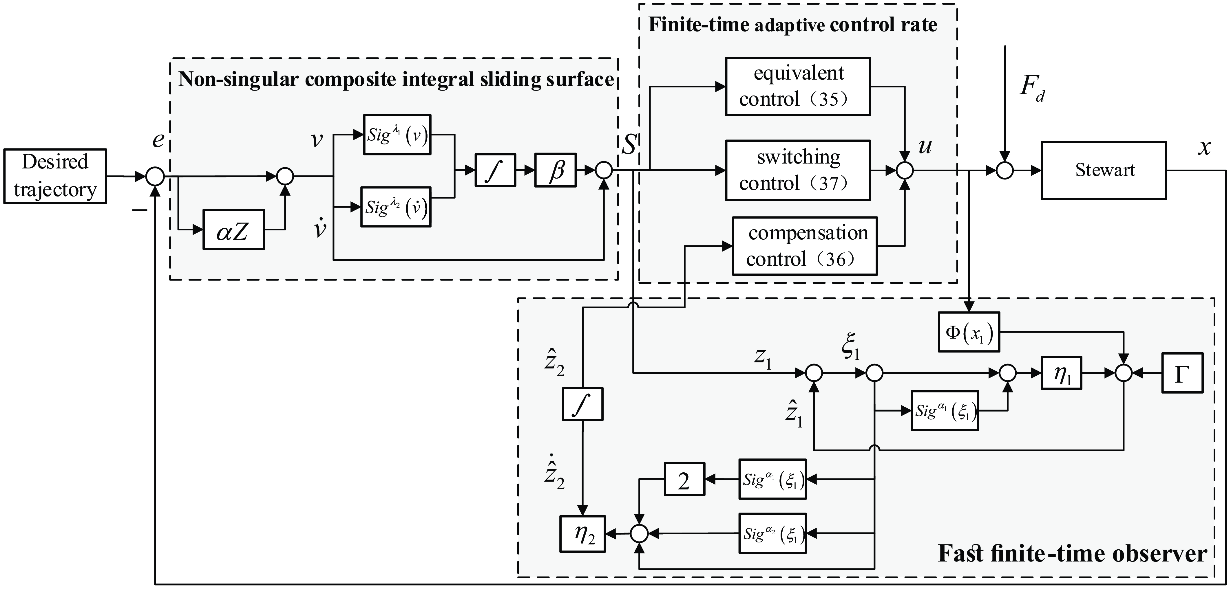
This section designs a Stewart platform finite-time adaptive sliding mode controller that adopts a nonsingular composite integral terminal sliding mode surface. It compensates for lumped uncertainties through a fast finite-time expansion state observer and designs an adaptive reaching law to reduce sliding mode chattering. The control system block diagram is shown in Figure 3.
Based on the proposed FFESO, the state-space expression of the Stewart platform can be rewritten as follows:
 \begin{equation} \left\{\begin{array}{l} \dot{x}_{1}=x_{2}\\ \dot{x}_{2}={\Phi} \left(x_{1}\right)u+f\left(x_{1},x_{2}\right)+z_{2}+\xi _{2} \end{array}\right. \end{equation}
where
 $\xi _{2}$
is the observation error. According to Theorem 2,
 $\xi _{2}$
converges to the stable region within a finite time
 $T_{3}$
. Therefore, it can be assumed that there exists a small normal constant
 $\xi _{d}$
that satisfies
 $\xi _{2}\leq \xi _{d}$
.
The proposed control scheme consists of three components: equivalent control, switching control, and lumped uncertainty compensation. It can be expressed as:
 \begin{equation} u=u_{eq}+u_{asw}+u_{d} \end{equation}
 \begin{equation} u_{eq}={\Phi} ^{-1}\left(x_{1}\right)\left(\begin{array}{l} \ddot{x}_{d}-f\left(x_{1},x_{2}\right)-\alpha G'\left(e\right)\dot{e}-\\[3pt] \beta \left(Sig^{{\lambda _{1}}}\left(v\right)+Sig^{{\lambda _{2}}}\left(\dot{v}\right)\right)-\xi _{d}b\left(S\right) \end{array}\right) \end{equation}
 \begin{equation} u_{d}=-{\Phi} ^{-1}\left(x_{1}\right)\hat{z}_{2} \end{equation}
 \begin{equation} u_{asw}={\Phi} ^{-1}\left(x_{1}\right)\left(-\frac{k_{1}}{\varphi \left(S\right)}b\left(S\right)-k_{2}h\left(S\right)S\right) \end{equation}
where
 $b\left(S\right)=\left\{\begin{array}{l} \frac{S}{\left\| S\right\| },\,\left\| S\right\| \neq 0\\ 0, \left\| S\right\| =0 \end{array}\right.$
is the norm-normalized sign function [Reference Li, Yu, Tee, Wu, Ge and Lee26], and
 $\varphi (S)=\varepsilon +(1-\varepsilon )e^{-c(| S| -1)} , h(S)=1-e^{-\lambda | S| } , k_{1}$
‵
 $k_{2}$
‵
 $\varepsilon$
‵
 $\mathrm{c}$
‵
 $\lambda$
are normal constants, as well as
 $k_{4}=k_{2}h(S)\gt 0$
and
 $k_{3}=\frac{k_{1}}{\varphi (S)}\gt 0$
.
It can be seen that when the system
 $| S_{i}|$
is far from the sliding surface,
 $\varphi (S_{i})\lt 1$
and
 $\nu (S_{i})$
approach 1, and at this point,
 $k_{3}=\frac{k_{1}}{\varphi (S)}\gt k_{1}$
and
 $k_{4}=k_{2}h(S)$
approach
 $k_{2}$
. The system will approach the sliding surface at a faster rate. Conversely, when
 $| S_{i}|$
approaches 0,
 $h(S_{i})$
approaches 0, and at this point,
 $k_{3}=\frac{k_{1}}{\varphi \left(S\right)}\lt k_{1}$
and
 $k_{4}=k_{2}h(S)$
approach 0, which reduces the gain and consequently reduces chattering.
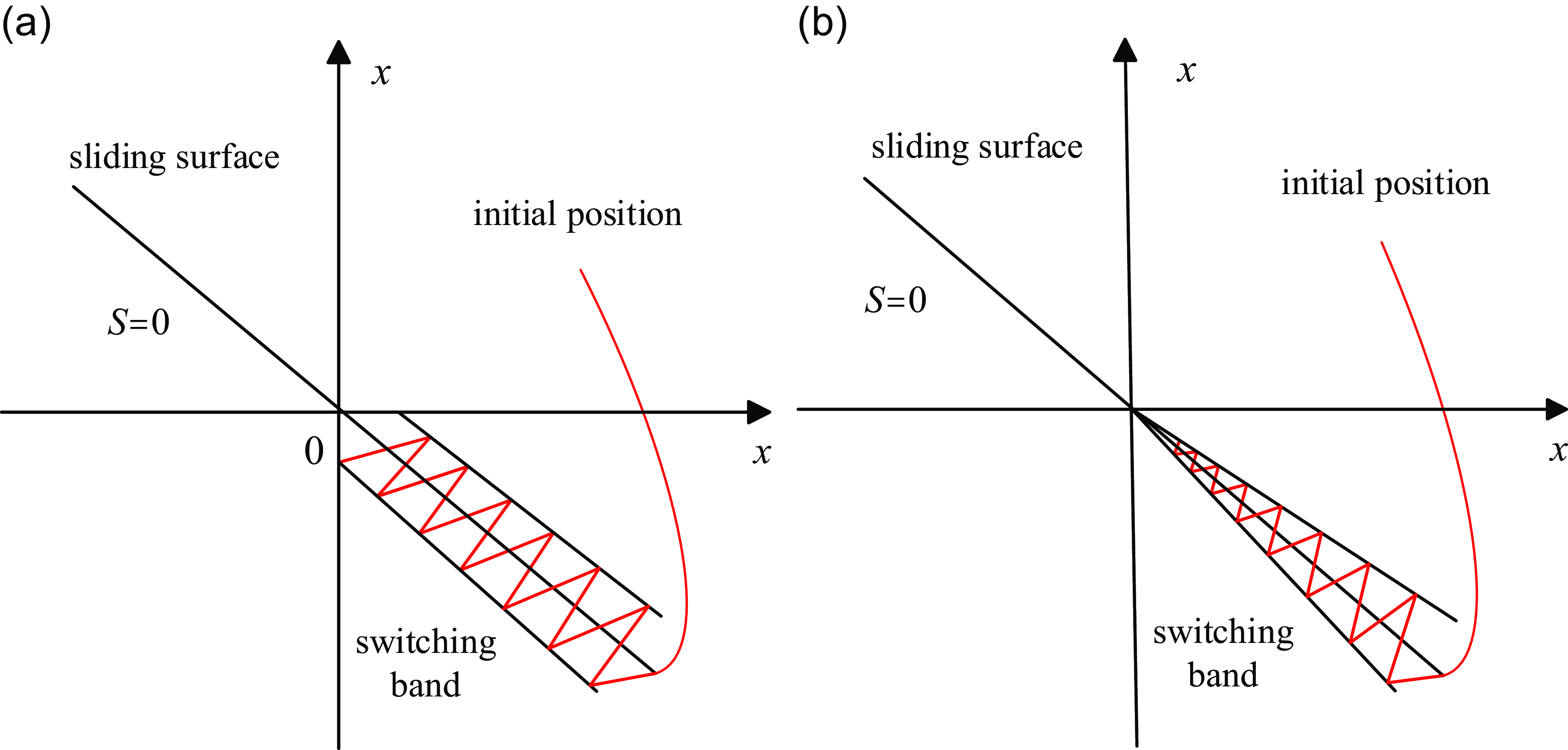
A comparison of the boundary layer sizes between the traditional exponential reaching law and the adaptive reaching law is shown in the following Figure 2. The proposed adaptive reaching law can dynamically adjust the approaching and sliding phase rates in real-time with changes in the sliding mode surface, solving the contradiction between approaching speed and chattering in the traditional exponential reaching law.
Phase plane graphs with different reaching laws. (a) Conventional exponential approach rate. (b) Adaptive approach rate.

Theorem 3: For the Stewart platform (4) with aggregated uncertainties, and by choosing the finite-time non-singular composite integral sliding mode surface (13) as mentioned above, using the proposed control rate (34), the entire closed-loop system is finite-time stable, and the position tracking error can converge to a small region near the origin within a finite time.
Proof: Consider the following Lyapunov function
 $V_{4}$
.
 \begin{equation} V_{4}=\frac{1}{2}S^{T}S \end{equation}
Take the derivative and substitute into the control rate (34):
 \begin{eqnarray} \dot{V}_{4} &=& S^{T}\left(\xi _{2}-\xi _{d}b\left(S\right)\right)-k_{3}\sum _{i=1}^{6}\left| S_{i}\right| -k_{4}S^{T}S\nonumber\\[0pt] &\leq& -k_{3}\sqrt{2}\left(\frac{1}{2}S^{T}S\right)^{\frac{1}{2}}-2k_{2}\frac{1}{2}S^{T}S\nonumber\\[0pt] &\leq& -\sqrt{2}k_{3}V_{4}^{\frac{1}{2}}-2k_{2}V_{4} \end{eqnarray}
where
 $\sqrt{2}k\gt 0$
and
 $2k_{2}\gt 0$
, according to Lemma 2, the sliding mode surface will converge to zero within a finite time
 $T_{4}$
. When
 $S=0$
, from Theorem 1, it is known that the position tracking error will converge to a neighborhood of zero within a finite time
 $T_{f}$
. Therefore, the position tracking error can converge within a finite time
 $T_{5}$
, denoted as
 $T_{5}\lt T_{\max }=T_{3}+T_{4}+T_{f}$
.
 \begin{equation} T_{4}\leq \frac{1}{k_{2}}\ln \frac{\mu _{1}V^{0.5}\left(S\left(0\right)\right)+\sqrt{3}k_{3}}{\sqrt{3}k_{3}} \end{equation}
3.4. Controller parameter selection
Unmodeled dynamics, external disturbances, and measurement noise in practical systems require an integrated selection of appropriate control parameters to balance control speed, accuracy, and signal smoothness.
-
1) Selection of Sliding Surface Parameters
 $\alpha , \beta , \lambda _{1} , \lambda _{2} , r , \kappa , m$
: The parameter
$\alpha$
affects the convergence rate of the tracking error, a larger
$\alpha$
leads to faster error convergence. However, an excessively large
$\alpha$
may result in increased control effort. An integral term in the sliding variable is introduced to suppress steady-state error, but an overly large integral gain
$\beta$
may induce steady-state deviation. Parameters
$\lambda _{1} , \lambda _{2}$
also influence the convergence rate and should satisfy
$0\lt \lambda _{1}\lt 1$
and
$\lambda _{2}=\frac{2\lambda _{1}}{\lambda _{1}+1}$
. Parameters
$r$
and
$\kappa$
are introduced to address the singularity problem, satisfy
$r\gt 1$
and
$m=1-\kappa$
, where
$\kappa$
is a small positive constant near the origin, satisfying
$0\lt \kappa \lt e^{-1}$
. In the experimental implementation, the following parameters were chosen:
$\alpha =10 , \beta =15 , \lambda _{1}=0.8 , \lambda _{2} , r=1.7 , \kappa =0.3 , m=0.7$
.
-
2) Selection of Parameters
$\eta _{1} , \eta _{2} , \alpha _{1} , \alpha _{2}$
: The parameters
$\eta _{1} , \eta _{2} , \alpha _{1} , \alpha _{2}$
determine the performance of the observer. In particular,
$\eta _{1}$
and
$\eta _{2}$
need to be sufficiently large to ensure satisfactory observation accuracy and convergence speed. The selection of
$\alpha _{1}$
and
$\alpha _{2}$
must also satisfy the conditions derived in the proof of Theorem 2 to guarantee system stability and estimation performance. In the experiments, the following parameter values were adopted:
$\eta _{1}=1500 , \eta _{2}=2000 , \alpha _{1}=0.8 , \alpha _{2}=0.6$
. -
3) Selection of Parameters
$\varepsilon , c , \lambda , k_{1} , k_{2}$
: The parameters
$\varepsilon , c , \lambda , \lambda _{2} , k_{1} , k_{2}$
are used to define the reaching law dynamics. Specifically,
$\varepsilon$
determines the convergence region of the tracking error. A smaller value of
$\varepsilon$
implies higher control precision; however, if
$\varepsilon$
is too small, it may cause control input saturation and induce chattering. Parameters
$k_{1}$
and
$k_{2}$
influence the convergence rate of the sliding motion, overly small values lead to slow convergence, while excessively large values may result in chattering. Therefore, proper tuning is essential. Parameters
$c$
and
$\lambda$
determine the adaptation rate in the adaptive law and must satisfy certain conditions
$0\lt c\lt 1$
and
$0\lt \lambda \lt 1$
. In the experimental implementation, the following values were selected:
$\varepsilon =0.1 , c=0.2 , \lambda =0.2 , k_{1}=10 , k_{2}=15$
.


Control System Block Diagram.

4. Simulation and experimental verification
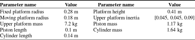
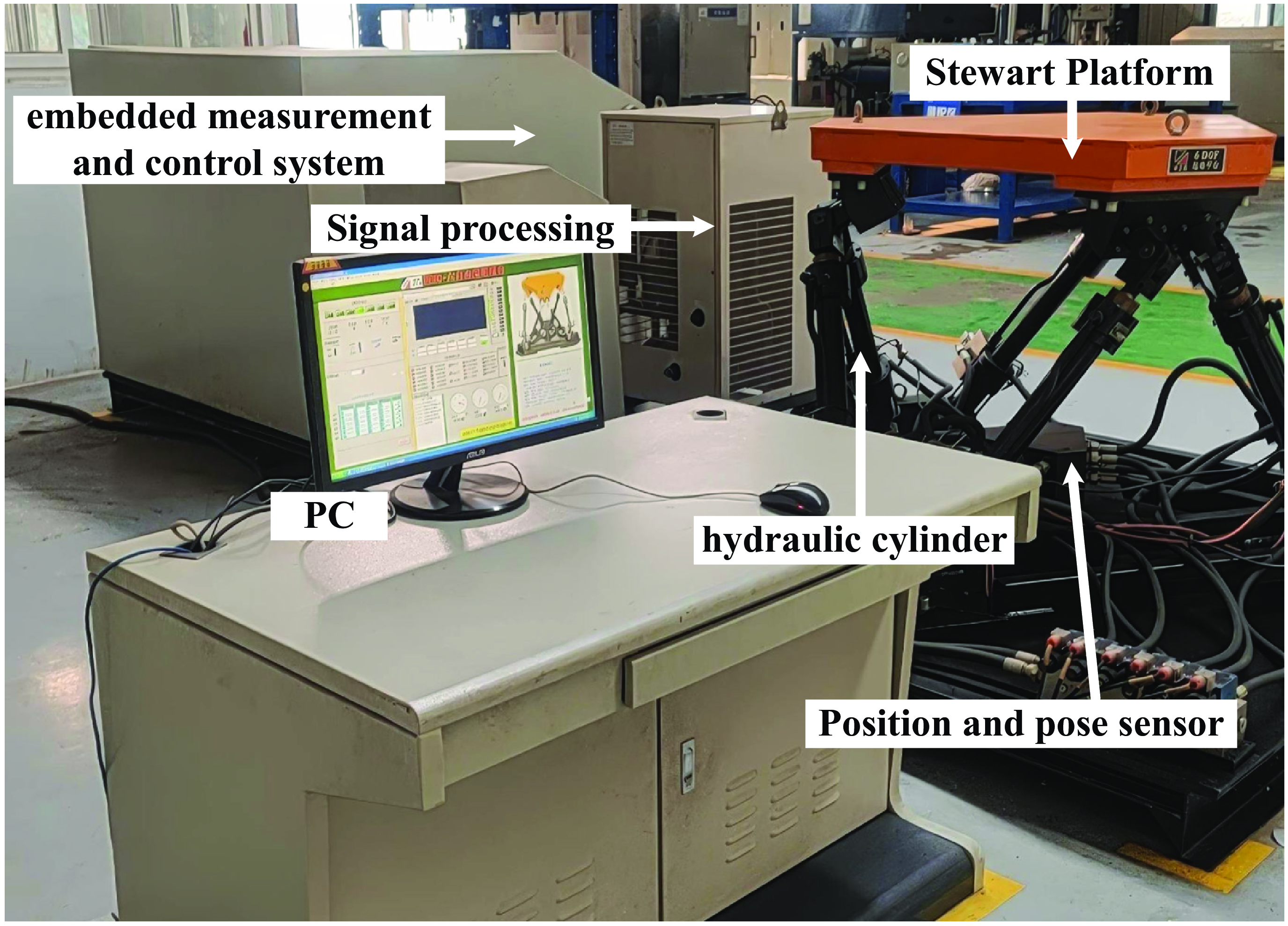
To verify the effectiveness of the controller design in this study, a combined simulation platform was built using SolidWorks and MATLAB. Simulation tests were conducted in MATLAB/Simulink, followed by physical verification on a hydraulic Stewart platform. The physical image of the Stewart platform is shown in Figure 4, and its main parameters are listed in Table I.
Stewart platform parameters.

4.1. Simulated analysis
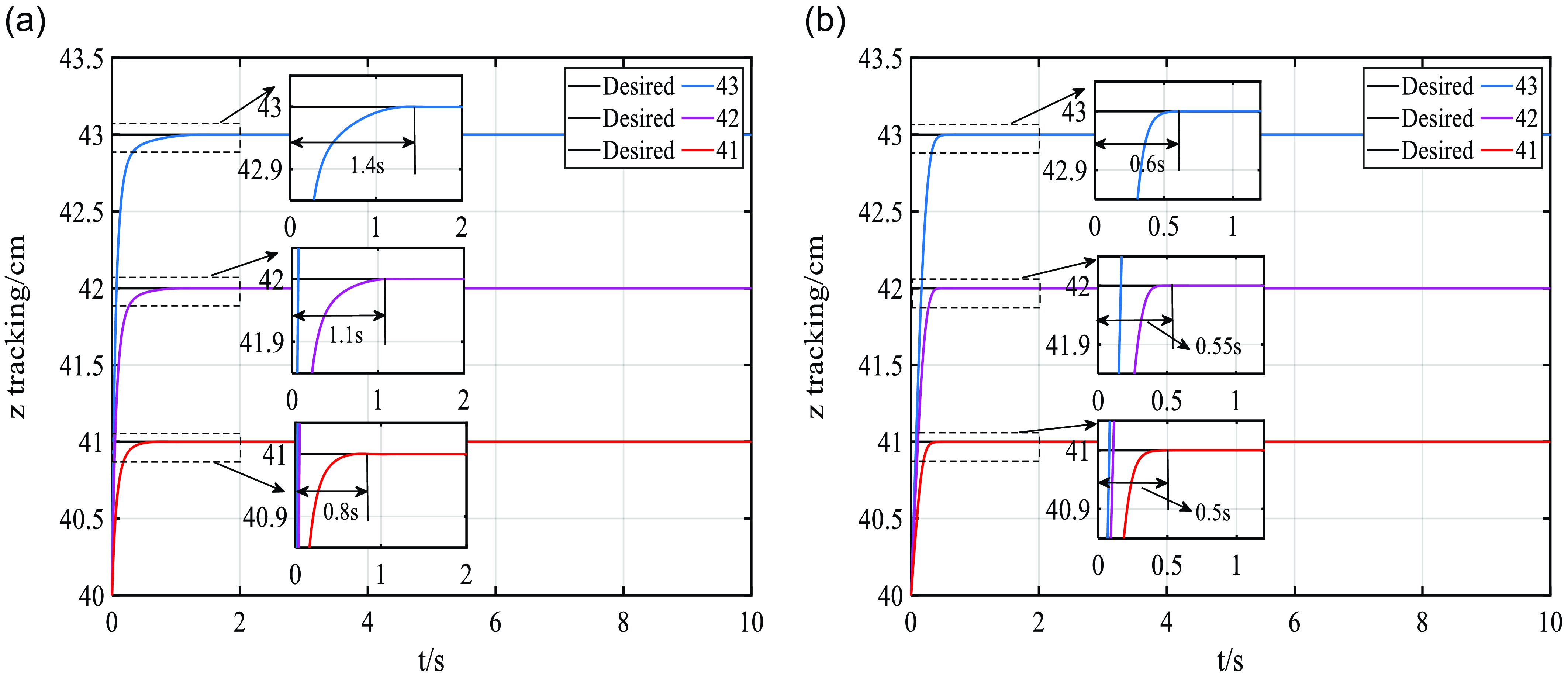
Finite-time control is a strategy aimed at driving the system from any initial state to the target state within a finite time. The initial state of the system often affects the control time, especially when the initial deviation is large, requiring more time for the controller to adjust the system. This paper proposes a globally finite-time convergent sliding mode surface composed of intermediate variables and integral terms. By designing appropriate initial values for the intermediate variables, the sliding mode reaching phase can be eliminated, reducing the impact of initial conditions on the controller.
The tracking trajectories of the z-axis are set to 41, 42, and 43 cm, with other conditions remaining the same. The tracking performance of the traditional integral sliding mode surface [Reference Asif, Khan and Memon27] and the proposed nonsingular composite integral sliding mode surface are shown in Figure 5, respectively. For the same tracking trajectory, by selecting
 $\alpha =10$
and
 $\beta =15$
, the proposed nonsingular composite integral sliding mode surface can eliminate the sliding mode reaching phase by setting the initial values
 $W(0)$
and
 $Z(0)$
in Eq. (13), thus resulting in a shorter convergence time than the traditional integral sliding mode surface.
Stewart experimental Platform.

To validate the performance of the proposed fast finite-time observer (FFESO), its observation performance was compared with that of the traditional ESO and the finite-time extended state observer (FESO) proposed in ref. [Reference He, Wu and Li28]. To test the observer’s observation accuracy and time, disturbances of 100N and 200N were added to the z-axis at 1s and 4s, respectively. The observer parameters
 $\eta _{1}=1500 , \eta _{2}=2000 , \alpha _{1}=0.8$
, and
 $\alpha _{2}=0.6$
were set, and verification was carried out.
The FFESO presented in this paper is designed based on a nonsingular composite integral sliding mode surface, enabling global finite-time convergence. Therefore, its convergence speed is faster than that of traditional observers, allowing for quicker estimation of total uncertainties. The results, as shown in Figure 6, indicate that the traditional ESO has poor observation performance and cannot accurately observe disturbances. The FESO can observe disturbances within 2 s, while the proposed FFESO can observe disturbances within 0.5 s, achieving a 75% improvement in convergence speed and more accurately estimating the magnitude of total uncertainty.
Comparison of initial conditions.(a) Traditional integral sliding surface (b) Non-singular composite integral sliding mode.

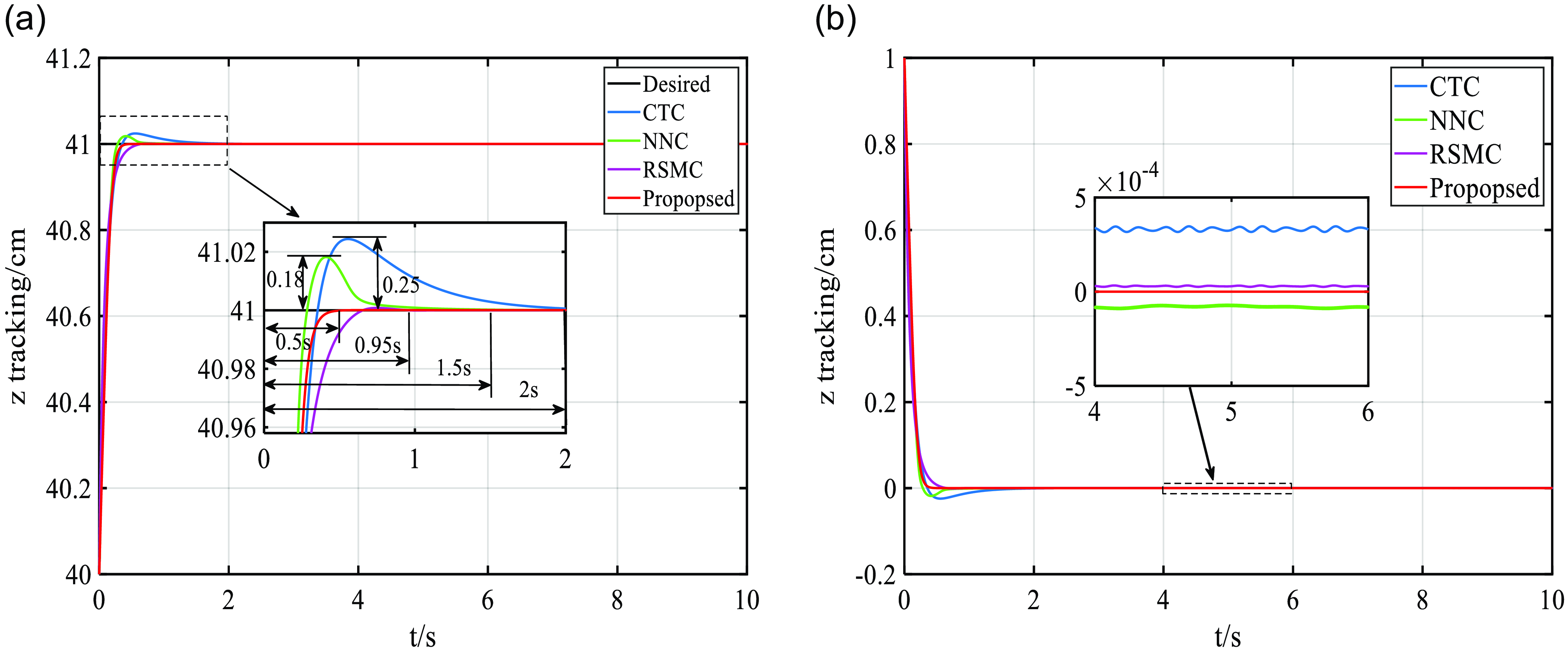
In order to fully demonstrate the superiority of the proposed sliding mode controller in terms of system convergence speed, stability, robustness, and control accuracy, a comparative analysis was conducted with traditional torque control (CTC) [Reference Dixon, de Queiroz, Zhang and Dawson29], neural network-based adaptive control (NNC) [Reference Chen, Ming and Qin30], and robust sliding mode control (RC) [Reference Xie, Yu and Chen31]. Firstly, to verify the control performance of the proposed method, step response comparisons of the z-axis were conducted for the four controllers. Time-varying disturbances
 $d=0.1\sin (20t-\pi /3)+0.2\cos (10\pi t)$
were introduced in the simulation to emulate unknown uncertainties, aiming to assess the effectiveness of the system in practical application scenarios. The proposed controller eliminates steady-state errors through NCISMS and quickly estimates disturbances using FFESO, resulting in higher convergence speed and accuracy compared to other control methods.
To evaluate the control performance of the proposed method, step response comparisons of the Z-axis under four different controllers were conducted. Time-varying disturbances were introduced in the simulation to emulate unknown uncertainties, aiming to assess the effectiveness of the system in practical application scenarios.
The tracking results are shown in Figure 7(a). The proposed controller exhibits no overshoot, with a convergence time of only 0.5 s, which is reduced by 75%, 67%, and 47% compared to the other three methods, respectively. The tracking error is shown in Figure 7. Due to the presence of the integral term, it significantly reduces the steady-state error, resulting in better control accuracy.
Comparison of Observation Results from Different Observers.

To further verify the robustness of the proposed method, a 300N disturbance is applied to the upper platform at 5 s to simulate an abrupt load.
The tracking results are shown in Figure 8. Compared to other methods, the proposed method has an overshoot of only 0.0002 cm, which is reduced by 99%, 80%, and 50% compared to CTC, NNC, and RC, respectively. The tracking error is shown in Figure 8, with a convergence time of 0.4 s, which is reduced by 84%, 67%, and 50%, respectively. This indicates that the proposed method has stronger robustness, as the fast finite-time observer and adaptive approach rate can effectively compensate for the impact of concentrated uncertainties on the system.
Step response of different controller. (a) tracking curve. (b) tracking error.

A further comparison of the combined tracking trajectory effect of the spiral ascent was conducted, considering 20% model uncertainty, i.e.,
 $M_{0}=0.8M , C_{0}=0.8C$
and
 $G_{0}=0.8G$
. The tracking trajectories of different controllers are shown in Figure 9. The results indicate that for complex trajectories, the proposed sliding mode controller has the smallest tracking error, still maintaining high-precision tracking and overcoming the impact of model uncertainties.
4.2. Comparison of tracking performance of different sliding mode controllers
To examine the trajectory tracking capability of the Stewart platform with six degrees of freedom, the reference trajectory is given as follows:
 \begin{equation} X_{d}\left(t\right)=\left\{\begin{array}{l} \sin \left(\pi t\right)cm\\[2pt] \cos \left(\pi t\right)\,cm\\[2pt] 0.2t+40\,cm\\[2pt] 0.1\sin \left(\pi t\right)\,rad\\[2pt] 0.1\cos \left(\pi t\right)\,rad\\[2pt] 0.1\sin \left(\pi t\right)\,rad \end{array}\right. \end{equation}
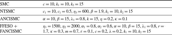
To verify the effectiveness of the proposed improved sliding mode control strategy, this section compares the proposed finite-time adaptive non-singular composite integral sliding mode control (FFESO-FANCISMC) based on a fast finite-time observer with traditional sliding mode control (SMC), the switching-type non-singular terminal sliding mode control (NTSMC) proposed in reference [Reference Fang, Cheng, Cheng and Fan32], and the non-singular composite integral sliding mode control with adaptive rate (ANCISMC) from reference [Reference Vo and Kang33], and performs experimental verification.
1) The design of the SMC is as follows:
 \begin{equation} S =\dot{e}+ce \end{equation}
 \begin{equation} u={\Phi} ^{-1}\left(x_{1}\right)\left(\begin{array}{l} \ddot{x}_{d}-f\left(x_{1},x_{2}\right)+c\dot{e}\\ -k_{1}sign\left(s\right)-k_{2}s \end{array}\right) \end{equation}
2) The design of the NTSMC is as follows:
 \begin{equation} S=\dot{e}+c_{1}G\left(e\right)+c_{2}Sig^{\beta }\left(e\right) \end{equation}
 \begin{equation} u={\Phi} ^{-1}\left(x_{1}\right)\left(\begin{array}{l} \ddot{x}_{d}-f\left(x_{1},x_{2}\right)-c_{1}G'\left(e\right)-\\[2pt] c_{2}\beta \left| e\right| ^{\beta -1}-k_{1}sign\left(s\right)-k_{2}s \end{array}\right) \end{equation}
3) The design of the ANCISMC is as follows:
 \begin{equation} u={\Phi} ^{-1}\left(x_{1}\right)\left(\begin{array}{l} \ddot{x}_{d}-f\left(x_{1},x_{2}\right)-\beta \left(Sig^{{\lambda _{1}}}\left(u\right)+Sig^{{\lambda _{2}}}\left(\dot{u}\right)\right)\\[2pt] -\alpha G'\left(e\right)-\left(\hat{\varphi }+\eta \right)sign\left(s\right)-ks \end{array}\right) \end{equation}
 \begin{equation} \hat{\varphi }=\frac{1}{\kappa }\left| S\right| \end{equation}
Controller parameters.

Step response of different controller(Load at 5s). (a) tracking curve. (b) tracking error.

Comparison of spiral upward tracking of different controllers.

Figure 13 shows the relationship between sliding mode switching gain and chattering. Apart from the switching gain, all other parameters are the same as those in the proposed method. It can be seen that chattering increases as the switching gain increases. In this experiment, parameters
 $k_{1}$
and
 $k_{2}$
were selected, with the other controller parameters specified in Table II
SMC exhibits significant oscillation and has a slow convergence rate. NTSMC improves the convergence speed through switching terms, and its transient response is better than SMC, but it still has steady-state error. ANCISMC uses the proposed NCISMS to eliminate steady-state error and adjusts the gain through adaptive coefficients, reducing oscillation to some extent, but sacrificing some convergence speed. The proposed FFESO-FANCISMC eliminates steady-state error through NCISMS, sets initial values to eliminate the sliding mode reaching phase, and improves system robustness through FFESO and adaptive rates. Figure 10 shows the trajectory tracking results of four sliding mode controllers, indicating that all controllers can smoothly complete the required position tracking. Figure 11 displays the tracking errors of different controllers. Compared to others, ANCISMC and the proposed controller have smaller steady-state tracking errors. The proposed controller has faster error convergence, smaller oscillations, and higher stability accuracy.
Relationship between the switching gain and chattering.

To better evaluate the performance of the proposed control scheme, this study uses two error-based performance metrics: Integral of Squared Error (ISE) and Integral of Time-weighted Absolute Error (ITAE), defined as follows:
 $ISE=\int _{0}^{t}e^{2}(t)d\tau , ITAE=\int _{0}^{t}t| e(t)| d\tau$
. The smaller the metric value, the better the control performance. The ISE and ITAE metric results for the trajectory tracking of different controllers are shown in Tables III and IV.
ISE of different controllers.

ITAE of different controllers.

Stewart experimental Platform.

By comparing the metric values in Tables III and IV, it can be easily concluded that the proposed controller has smaller ISE and ITAE values than other methods. For example, for axis tracking, the ISE value of the proposed controller is 12.3% of the SMC, 33.9% of the NTSMC, and 37.2% of the ANCISMC, representing a reduction of 87.7%, 66.1%, and 62.8%, respectively. The ITAE value of the proposed controller is 25.4% of the SMC, 42.4% of the NTSMC, and 44.5% of the ANCISMC, representing a reduction of 74.6%, 57.6%, and 55.5%, respectively. In both transient and steady-state responses, the proposed finite-time adaptive sliding mode controller can achieve superior tracking performance compared to other controllers.
Figure 12 shows the control inputs for tracking the trajectories of the six legs. It can be seen that the chattering amplitude of SMC is 3N, while the switching-type nonsingular terminal sliding mode control and the nonsingular composite integral sliding mode control with adaptive rates can reduce the chattering of SMC to some extent, with chattering amplitudes of 2.5N and 1.5N, respectively. The method proposed in this paper uses a fast finite-time extended state observer, which can more accurately estimate the magnitude of both internal and external lumped uncertainties. At the same time, the use of adaptive approaching rates significantly reduces the chattering phenomenon, with a chattering amplitude of only 0.2N. Compared to other methods, this reduces the chattering by 93.3%, 92%, and 86.7%, respectively. Therefore, the designed controller has smaller chattering and can track the desired trajectory more accurately, achieving high-precision tracking control for the Stewart platform.
6-DOF trajectory tracking error.

To fully verify the robustness and finite-time convergence of the proposed method, trajectory tracking tests were conducted under three different conditions: no load, 10 kg load, and 30 kg load, following a given reference trajectory
 $X_{d}(t)=\{2\sin (\pi t),2\cos (\pi t),41,0,0,0\}$
. As shown in Figure 14, the proposed control strategy demonstrates excellent trajectory tracking performance under all load conditions, further confirming its strong robustness and fast response capability.
Control Input.

5. Conclusion
This paper proposes an adaptive non-singular composite integral sliding mode control strategy based on a fast finite-time observer for achieving finite-time high-precision tracking control of a Stewart parallel robot in the presence of model uncertainties and external disturbances. The following conclusions are drawn from the simulation and experimental results:
-
(1) The proposed NCISMS, through intermediate variables and integral terms, can achieve global finite-time convergence and eliminate steady-state errors.
-
(2) The FFESO proposed based on NCISMS can more accurately estimate the magnitude of both internal and external lumped uncertainties, improving the system’s robustness.
-
(3) Compared with other methods, the improved method FFESO-FANCISMC presented in this paper solves the contradiction between the convergence speed and chattering in the traditional exponential approaching law. Its trajectory tracking demonstrates faster dynamic response and higher stability, significantly suppressing chattering phenomena and achieving fast and accurate trajectory tracking within a finite time.
In practical applications, complex working conditions may involve high-frequency measurement noise and non-ideal actuator characteristics. Furthermore, potential actuator and sensor faults must also be considered. Therefore, our future research will focus on developing fault-tolerant control strategies based on sliding mode theory. We aim to conduct experimental validations under more challenging task conditions, along with more comprehensive theoretical analysis and experimental studies, to enhance the feasibility and robustness of the proposed method in more complex real-world scenarios.
XY-plane trajectory tracking plots under different loads.

Author contributions
Xingyu Qu and Jiasheng Zhai conceived and designed the study. Jiasheng Zhai and Chengxiang Qiao conducted data gathering and performed statistical analyses. Jiasheng Zhai wrote the article.
Financial support
This research received no specific grant from any funding agency, commercial or not-for-profit sectors.
Competing interests
The authors declare no conflicts of interest exist.
Ethical approval
Not applicable.