Introduction

One explanation for the North Atlantic’s Heinrich layers is that the Hudson Bay portion of the Laurentide ice sheet repeatedly expelled large quantities of its mass into the North Atlantic because of ice-sheet instability (Reference MacAyealMacAyeal, 1993a, Reference MacAyealb). A post-Heinrich Laurentide ice sheet would have a significantly lower surface. In this paper, the possible connection between variability in the Greenland climate record and the topographic variations of the Laurentide ice sheet, that may describe ice-sheet control on the atmosphere’s stationary wave patterns, is explored.

Models of ice-age atmospheric circulation have typically focused on the average glacial climate without regard to the many climate fluctuations that are indicated in the climate record. This is mainly due to the sparsity of geologic data used to constrain model boundary conditions such as sea-surface temperature and ice-sheet topography. Modeling glacial climate variability presents unique difficulties since sea-surface temperature and ice-sheet topography may not be static. The study of Heinrich events present such a difficulty, since the geologic record does not specify how such boundary conditions were changing. Presented here is an examination of the sensitivity of a model atmosphere’s stationary wave field to changes in ice-sheet topography. The goal is to show how one boundary condition in particular can elicit climate variability.

An idealized two-layer atmosphere is modeled on a spherical Earth to approximate the behavior of the real atmosphere. Particular features of the model’s behavior may not be realistic. However, the modeling exercise still provides a general lesson on how glacial climate variability may relate to changing ice-sheet conditions. No attempt is made to study the effects of sea-surface temperature and its variability on glacial climate.

Model Formulation

Each of the two layers is modeled using the “shallow-water” approximation and the momentum-balance equations for incompressible fluid flow. Each layer’s flow is independent of height and has a constant density. The upper layer is slightly less dense than the lower layer, and their common interface is allowed to change its elevation as a means of coupling the two layers.

Winds in the two-layer model arise from heating in the tropics and cooling at high latitudes. While the atmosphere accomplishes this diabatic forcing through radiative and microphysical processes, a two-layer model simulates the effect of healing by a thickening of the upper layer. Conversely, a thinning of the upper layer simulates the effect of cooling. The thickness of the upper layer is forced to a “radiative equilibrium” profile by a Newtonian relaxation scheme with a 30 day radiative time-scale. Frictional damping of momentum occurs in the lower layer by a Newtonian relaxation scheme that damps wind velocities with a 10 day frictional time-scale.

The temperature of a two-layer section of atmosphere can be calculated once a global averaged temperature is specified. The deviation from this global mean takes into account the relative thickness of each layer as well as the density difference between each layer. The present model contains a 50°C temperature difference between the poles and the equator.

The governing equations are solved on a sphere using the spectral transform method with a R30 truncation. The corresponding resolution of the truncation is 7.5° longitude and 4.5° latitude grid spacing.

Initial tests of the two-layer model’s circulation over the Himalaya and Rocky Mountains revealed symptoms of super-rotation in which the model’s Northern and Southern Hemisphere jet streams migrated and joined together along the Equator. Previous studies of two-layer models suggested this tendency may be remedied by introducing vertical diffusion of momentum between the two model layers (Reference SaravananSaravanan, 1993). In the current research, a Newtonian relaxation scheme was used to adjust locally one layer’s momentum toward the other layer’s value with a 20 day time-scale. This change was sufficient to remedy the emergence of super-rotation.

There are two indications that the two-layer model behaves reasonably well. One indication stems from its ability to produce realistic zonal flow. The time-averaged zonal flow with symptoms of super-rotation removed contains mid-latitude upper-level jets, weaker lower-level flow, and weak tropical easterlies. These features are in general agreement with observations.

The second indication of the model’s good behavior is its ability to reproduce some features of the observed time-averaged flow over the Rocky Mountains and Himalaya. The model produces a stream-function field giving fluid velocity measurements that, in the time average, contains wavelike disturbances or stationary waves associated with flow over topography. The model was able to reproduce the amplitude and longitudinal extent of the stationary wave in the lee of the Rocky Mountains. The model had some difficulty in reproducing the amplitude and longitudinal extent of the stationary wave in the lee of the Himalaya. Since the present model does not contain thermally driven circulation from land-ocean temperature contrasts or latent heat release from precipitation, an exact matching between model and the atmosphere is not to be expected.

Experiment Design

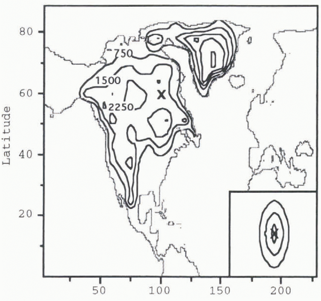
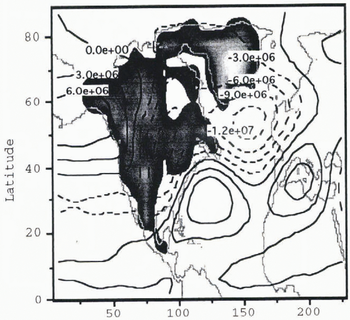
The Heinrich-event simulation is composed of two separate model experiments. The first (pre-Heinrich) event experiment calculates the stationary wave response of the model atmosphere to the Reference PeltierPeltier (1994) ICE-4G reconstruction of the Last Glacial Maximum Laurentide and Greenland ice sheets (Fig. 1). The model saves the stream function every 12 hours for the upper and lower layers for a 90 day period. These data become averaged together by layer, and zonal averages are removed to leave the stream-function perturbation field. The total stationary wave is defined to be the av erage of the upper- and lower-layer stream-function per-turbations.

Fig. 1.

Contour plot of pre-Heinrich-event Laurentide and Greenland ice-sheet topography. Contour intervals are 750 m. The ‘X’ mark on the ice sheet corresponds to the location of maximum ice loss that will be present following a Heinrich event. The geometry of the mass removed is given in the box in the lower right corner. Contour intervals in the box are also 750 m.

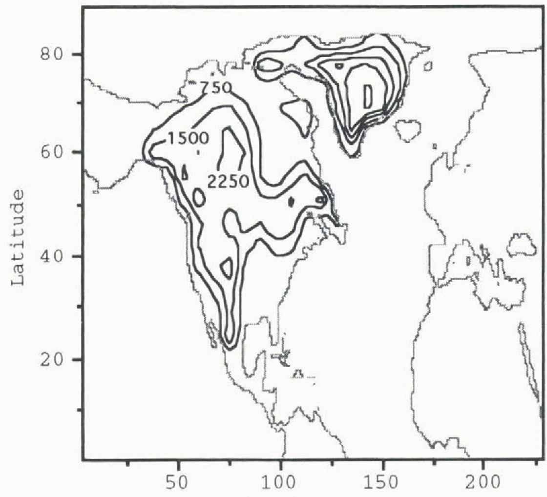
The second (post-Heinrich event) experiment calculates the stationary wave field created by a post-Heinrich-event Laurentide and Greenland ice sheets (Fig. 2). This topography is created by removing 10⁶ m³ of ice from the portion of the Laurentide ice sheet covering Hudson Bay. Estimates of the amount of ice involved in a Heinrich event are calculated from the amount of debris found in the North Atlantic’s sediments (Reference Alley and MacAycalAlley and MacAyeal, 1994). The value used here is within the uncertainty of this estimate.

Fig. 2.

Contour plot of post-Heinrich-event Laurentide and Greenland ice-sheet topography. Contour intervals are 750 m.

Results

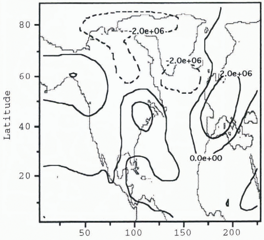
Figure 3 shows the stationary stream-function perturbation in the model atmosphere to a pre-Heinrich ice-sheet configuration before the removal of the Hudson Bay ice dome. Negative values of in Figure 3 indicate zonal-flow deviations in a cyclonic (counter-clockwise) direction. One may see from Figure 3 the minimum contour occurs southeast of the Laurentide ice-sheet’s midsection and extends across the North Atlantic. The effect of the ice topography is to force local polar air southward. In this manner, ice sheets are thought to force a mechanical cooling of the North Atlantic. A similar distribution and magnitude of is also apparent in the post-Heinrich-event ice-sheet atmosphere (Fig. 4). There are, however, notable differences over the North Atlantic.

Fig. 3.

Pre-Heinrich event atmosphere stream function perturbation Contour intervals are 3 × 10⁶ m² s⁻¹. The gray shading shows the geometry of the pre-Heinrich-event ice sheet given in Figure 1.

Fig. 4.

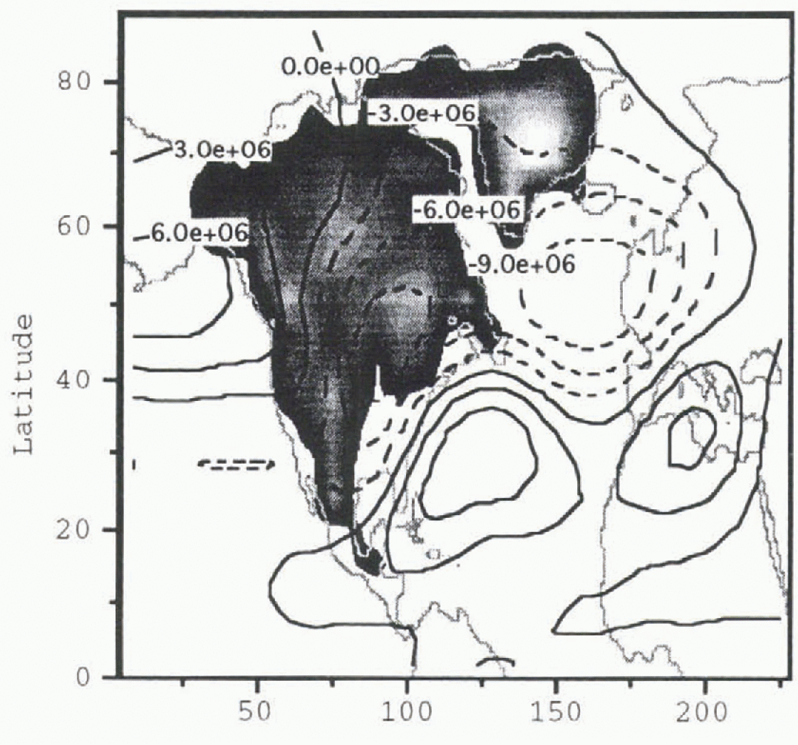
Post-Heinrich-event atmosphere stream-function perturbation Contour intervals are 3 × 10⁶ m² s⁻¹. The gray shading shows the geometry of the post-Heinrich-event ice sheet given in Figure 2.

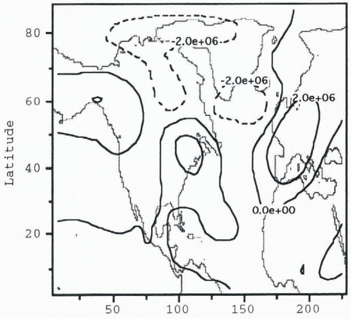
The difference in 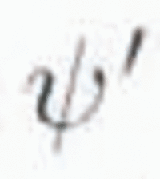between the two experiments (post- minus pre- ) over the North Atlantic is shown in Figure 5. The difference has a large negative amplitude over the North Atlantic. The interpretation is that the removal of the Hudson Bay ice dome augmented the stationary wave in the vicinity of the North Atlantic. The amplitude of the change is significant, reaching more than 30% of the pre-Heinrich-event stationary-wave amplitude. 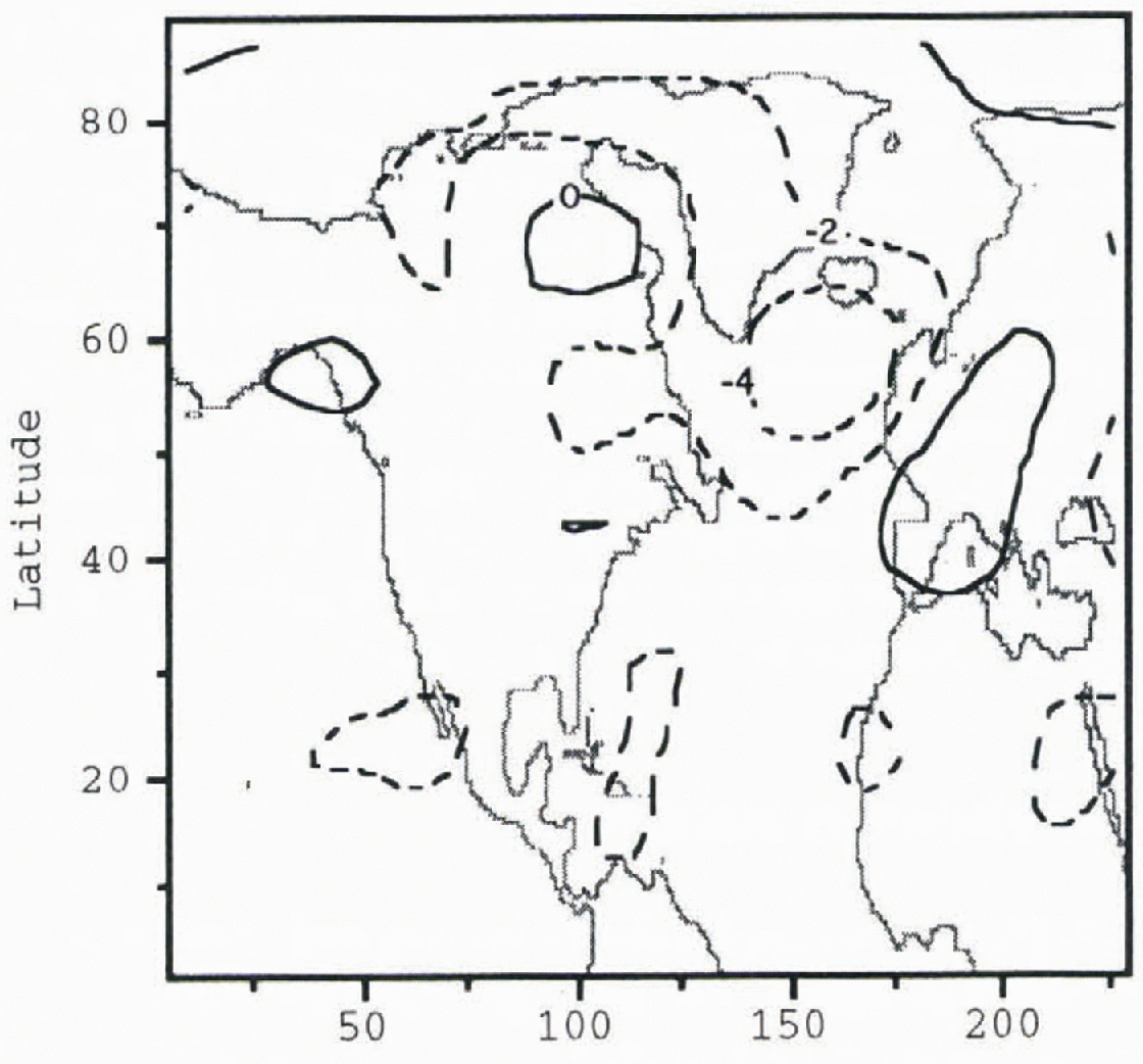The magnitude of this effect can be appreciated through changes in the model’s time-averaged temperatures, which indicate a 4°C cooling over much of the North Atlantic (Fig. 6).

Fig. 5.

Difference in between the pre-Heinrich-event experiment and the post-Heinrich-event experiment (Fig. 4 minus Fig. 3). Contour intervals are 2 × 10⁶ m² s⁻¹.

Fig. 6.

Difference in column-averaged temperatures between the pre-Heinrich-event experiment and the post-Heinrich-event experiment (post-Heinrich-event temperature field minus pre-Heinrich-event temperature field). Contour intervals are 2°C

Discussion

The results are surprising since the removal of some of the mass of the Laurentide ice sheet led to further cooling over the North Atlantic. This result suggests that stationary wave contributions from different sections of the Laurentide ice sheet were adding together destructively, or were being controlled by nonlinear terms. Stationary wave theory is limited and does not offer much intuition into this model observation. One expects from linear-geostrophic theory applicable to a single-layer constant-density atmosphere that the amplitude of a topographically forced stationary wave should be related to the topography’s volume. Decreasing a mountain’s volume should lead to a smaller stationary wave. The results of this paper’s simulations demonstrate the opposite. However, this may be because the longitudinal extent of the Laurentide ice sheet is sufficiently long to be comparable to the stationary wavelength where destructive interference, in the sense of linearized single-layer models, may be important. The stationary waves of a two-layer model might be entirely different, since stationary waves only exist as a time-averaged statistic. Further tests are needed to determine the mechanism(s) behind the model’s results, including an investigation into the idea of destructive interference of stationary waves by conducting a series of simulations with idealized topography with simple geometries. Both single-layer and two-layer model experiments with idealized topography should be illustrative of how stationary waves from different wave sources interact.

The two-layer model results suggest the Laurentide ice sheet’s altered topography could be reflected in the geologic record. However, since no attempt has yet been made to reveal why these results have arisen, some caution should still be exercised. The results might be an artifact of unrealistic model performance.

A possible extension of the Heinrich-event experiment is to explore the sensitivity of the stationary wave field to other sections of the ice sheet. One possibility is to investigate the influence of an ice dome over the eastern edge of the Canadian continental shelf, the portion in close association with Cabot Strait, to see if variable topography there would leave its own climate signature.

Conclusion

A two-layer model of atmospheric circulation has been used to evaluate the change due to the collapse of the Hudson Bay ice dome. The model shows a counter-intuitive result in that the amplitude of the ice-sheet forced stationary wave is increased by the removal of the Hudson Bay ice dome. The size of the change is large enough to show up in the geologic record. This result is relevant to the interpretation of climate records of the last ice age, and also implies that it may be possible to obtain more detailed information about ice-sheet topography from alternate climate proxy data sources. However, the results of this experiment are only preliminary and await further validation.