1.0 INTRODUCTION
In recent years, there has been an increasing trend towards the design and development of nanosatellites. They are cost effective and are often launched as secondary payloads with larger spacecraft. The first nanosatellite, developed by California Polytechnic State University (Cal Poly) in collaboration with Stanford University, is called CubeSat with dimensions 10×10×10 cm3 and mass less than 1.33 kg(Reference Munakata1). This has opened a window of research for universities and Small and Medium Enterprises (SMEs) worldwide in the field of nanosatellites.
The Department of Electronics and Telecommunication (DET) at Politecnico di Torino has been working on a comprehensive nanosatellite project called AraMiS (Italian acronym for Modular Architecture of Satellites) since 2007(Reference De Los Rios, Roascio, Reyneri, Sansoè, Passerone, Del Corso, Bruno, Hernandez and Vallan2). The design process of AraMiS is based on the concept of tiles and modules(Reference Mughal, De Los Rios, Reyneri and Ali3,Reference Mughal, Ali and Reyneri4) . These modules can be reused for multiple missions, which help to significantly reduce the overall cost, development and testing time(Reference Speretta, Reyneri, Sanso´e, Tranchero, Passerone and Del Corso5). One has to just reassemble the required sub-systems to achieve the targeted specific mission. AraMiS-C1 is a 1U CubeSat standard nanosatellite, developed by the DET as a demonstrator of the AraMiS modular architecture. Six faces of the satellite are equipped with identical “tiles” called CubeSat Power Management Tile (CubePMT). Inside the satellite, there is room for batteries and payload boards. Solar panels are fixed and mounted on six external surfaces.
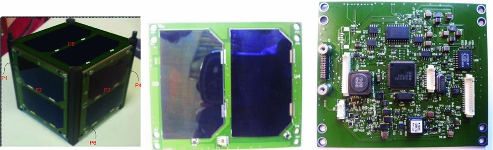
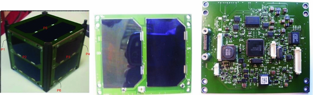
CubePMT is a power management, attitude determination and control tile of AraMiS-C1(Reference Ali, Reyneri, De Los Rios and Ali6,Reference Ali, Mughal, Ali and Reyneri7) . It is built on eight layers of FR4 Printed Circuit Board (PCB) with dimensions 98×82.5×1.6 mm3, which also acts as the mechanical structure of the satellite. The solar panel and sun sensor are mounted on the external side (layer 1) while power and attitude sub-systems are mounted on the internal side (layer 8). A magnetorquer coil with 200 turns is integrated within the PCB's four internal layers (layers 2, 3, 4 and 5)(Reference Ali, Mughal, Ali, Reyneri and Aman8). Layer 6 has the ground plane while Layer 7 contains partial ground planes. Photographs of the CubePMT solar panel and component side are shown in Fig. 1.
Photographs of AraMiS-C1 and CubePMT module.
A comprehensive and precise thermal analysis is an essential element in the development cycle of small satellites. Thermal control is critical to the success of any spacecraft mission, and without a proper thermal control system, the extreme temperature variations during flight may exceed component operating temperature ranges, leading to performance degradation or even permanent damage. On the other hand, NASA's Guidelines for Satellite's hardware thermal analysis warns that a conventional thermal control system may need extra space, power and, furthermore, to increase the overall weight of the satellite(9). The CubeSats are very attractive for universities and SMEs because of their short development times, lower development cost and relative simplicity compared to big satellites. However, due to the limited size, thermal control may be more difficult than with their larger counterparts. Smaller surface area provides less space for radiators and solar panels, as well as less thermal paths and interfaces for radiators or other thermal control hardware. It means that adding active thermal control systems to small satellites is not a suitable solution for their thermal control. The proper solution is the passive one, i.e. by making small satellite structure suitable for efficient heat dissipation. This paper provides a thermal modelling technique for analysing the satellite's structure as a network of thermal resistances.
This paper includes the following sections. Section 2 discusses the background and literature review while Section 3 discusses the methodology for detailed and simplified generic thermal model of the CubeSat and its panels. In Section 4, the thermal modelling presented in Section 3 is applied to AraMiS-C1 and its panels and their thermal resistances are measured. In Section 5, the thermal resistances evaluated via the thermal models presented in Section 3 are verified through laboratory experiments. The measurements regarding the absorbed power and the corresponding temperature differences between different points of the single panel and complete satellite are described in Section 6. The last Section 7 concludes the paper. The paper is basically based on the work Dr. Anwar Ali did during his PhD research(Reference Ali10).
2.0 BACKGROUND & LITERATURE REVIEW
Heat is generated by the satellite sub-systems as well as absorbed from the environment. In space, heat transfers through conduction and radiation; there is no convection heat transfer(11). Therefore, the satellite face in front of the sun has higher temperature, while the opposite side has a very low temperature. The temperature difference between the hot and cool face depends on the thermal resistance of the satellite. If the satellite material has a high thermal resistance, heat does not quickly dissipate to the cooler face and is trapped in the hotter side of the satellite which increases further the sub-systems temperature mounted on that side. The high temperature degrades the performance and reduces the lifetime of the satellite sub-systems. The thermal resistance is related to the spacecraft structure material and the design dimensions.
2.1 Temperature difference
When an object is exposed to the sun, some portion of the solar power is absorbed by the object and the remaining power is reflected back from the object surface. Absorbed power (P) is given by Equation (1).
 $$\begin{equation}
P = \alpha \cdot {P_d} \cdot S,
\end{equation}$$
where α is the absorption coefficient of the exposed surface, Pd is the solar power density, S is the exposed surface area and P is the power absorbed by the surface.
When solar panels are exposed to the solar power, they absorb some portion of the incoming solar power and the remaining power is transmitted to the satellite sub-systems. The power absorbed by the solar panel is transformed to useful power where as the power transmitted to the satellite is stored as unwanted heat power. The unwanted power (Pu ) depends on Pd , solar panel conversion efficiency (η), absorption coefficient (α), and S, given by Equation (2).
 $$\begin{equation}
{P_u} = {P_d} \cdot S \cdot (1 - \eta ) \cdot \alpha
\end{equation}$$
Based on the analogy between thermal and electrical networks with the respective components and parameters, in thermal domain, Ohm's law(12) is given by Equation (3).
 $$\begin{equation}
\Delta T = P \cdot {\theta _{th}},
\end{equation}$$
where ΔT is the temperature difference across an object, P is the power dissipated and θ th is the thermal resistance which can be found using the Fourier's Law for heat conduction(13).
2.2 Thermal model
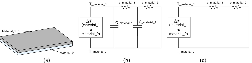
Thermal systems can be modelled as a network of thermal resistances and thermal capacitors. Suppose that an object is composed of two materials attached with each other as shown in Fig. 2.
(a) Object composed of two materials (b) Transient thermal model (c) Steady state thermal model.
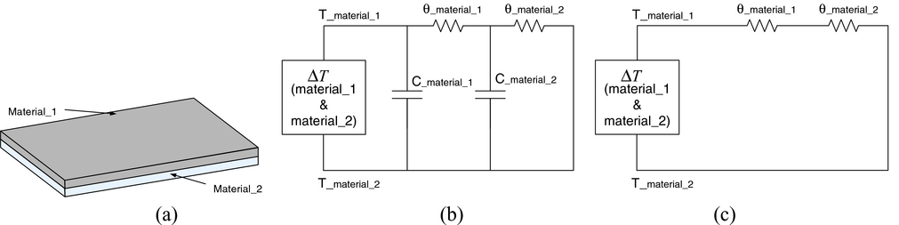
The transient and steady state thermal models between the top surface of material_1 and bottom surface of material_2 for the object shown in Fig. 2(a) are given in Fig. 2(b) and (c), respectively. Where ΔT is the temperature difference between material_1 and material_2; T_material_1 is the top surface temperature of material_1; T_material_2 is the bottom surface temperature of material_2; θ_material_1 is the thermal resistance of material_1; θ_material_2 is the thermal resistance of material_2; C_material_1 is the thermal capacitance of material_1; and C_material_2 is the thermal capacitance of material_2.
The transient thermal model is composed of both thermal resistances and thermal capacitances of the respective materials. In the steady state model, when the power and temperature reach the constant levels, the thermal capacitors are fully charged and can be neglected from the thermal model as shown in Fig. 2(b).
Thermal modelling has immense importance in the structural design of small satellites; therefore, various attempts have been made to accurately present thermal models of small satellites. In Ref. Reference Richmond14, the Adaptive Thermal Modelling Architecture (ATMA) has been discussed which focuses to bridge the gap between the commercially available thermal modelling tools used for larger, more expensive satellites, and the low-fidelity algorithms and techniques used for simple first order analysis. Work in Ref. Reference Moffitt and Batty15 addresses thermal modelling used during the design and analysis of the Combat Sentinel Satellite (CSSAT). An overview of the analysis is used to make design decisions and create working thermal models. In Ref. 16, thermal models of various spacecraft sub-systems have been created using MatLab and used to simulate projected operational modes of the satellite and the effects on major satellite sub-systems. As compared to all the previously developed models, our presented model is very simple, accurate, and robust which requires no special tool. The model is composed of detailed and simplified models for CubeSat and its panels.
3.0 METHODOLOGY
3.1 Thermo-mechanical model of the CubeSat panel
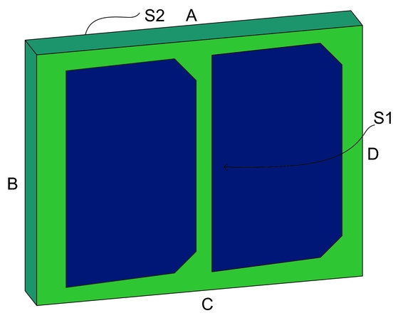
Normally on CubeSat, six faces are equipped with identical panels that are dual purpose: generating power as well as providing mechanical structure of the satellite. These panels are combined into a cube structure with the help of aluminum rails. The thermo-mechanical model of the CubeSat panel is shown in Fig. 3.
Thermo-mechanical model of CubeSat panel.
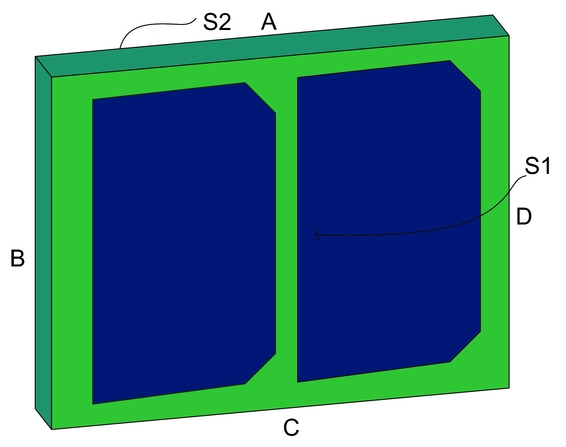
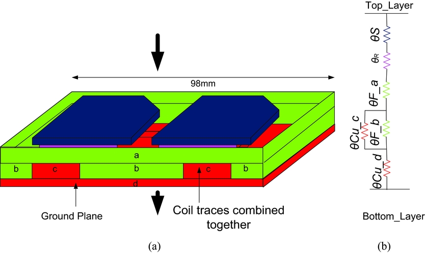
The generalised thermal models have been presented for a generic CubeSat panel. The composition of materials and dimensions of the CubeSat panel may vary from satellite to satellite. Here, it is assumed that the CubeSat panel under discussion is composed of solar cells, resin, FR4 and copper materials. For simplification and better understanding, the thermo-mechanical model of the CubeSat panel shown in Fig. 3 is sub-divided further into three portions and corresponding detailed and simplified thermal models for the three portions of the CubeSat panel are presented.
3.1.1 Top-to-bottom thermal model of the CubeSat panel
The top-to-bottom thermal (S1 to S2 face) model of the CubeSat panel shown in Fig. 3 has been found using detailed and simplified models. In the detailed model, thermal resistances associated with each sub-section are presented, while in the simplified model, the different sub-sections of similar material are merged and represented with a single resistor. Therefore, in the simplified model, the computation becomes easier because the total number of resistors is reduced.
3.1.1.1 Detailed thermal model
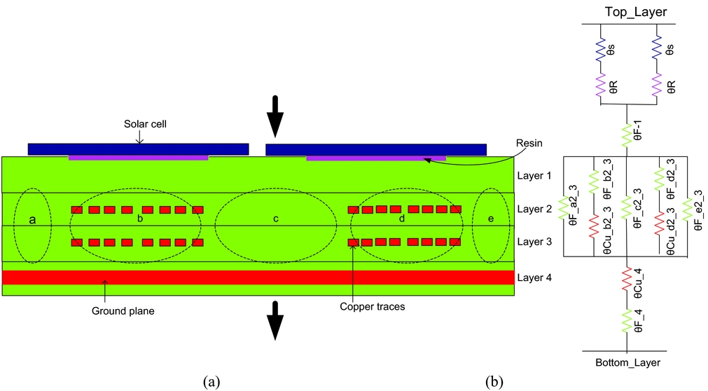
The cross-sectional view of the generalised structure of CubeSat panel and the corresponding detailed thermal model are shown in Fig. 4(a) and (b) respectively. The CubeSat panel under consideration is composed of four layers of FR4 PCB. The solar cells are attached on layer 1 using a thermally conductive resin as highlighted in Fig. 4(a). Layers 2 and 3 are embedded inside FR4 and have different layers of copper traces of certain dimensions. The internal layers may have different numbers of copper traces of certain dimensions. Layer 4 has the ground plane.
CubeSat panel (a) cross-sectional view (b) detailed model.
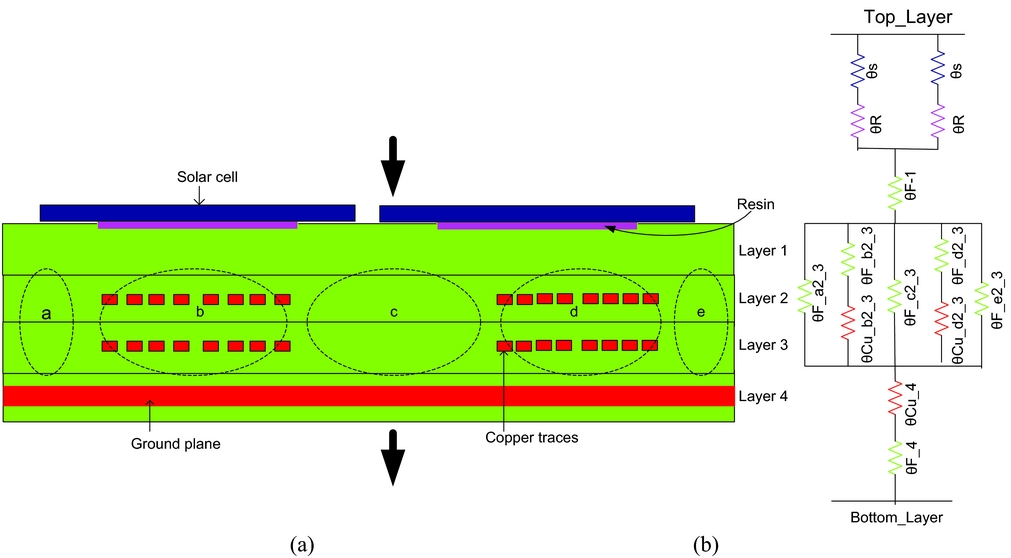
In order to get a detailed model, the panel has been divided into different sub-sections with respect to the type of material. Each sub-section has an associated thermal resistance, as depicted in the detailed model of Fig. 4(b). The value of the thermal resistance depends on the length, width and material type of the respective sub-section. In the detailed model, the solar cell resistance (θs) is in series with its resin resistance (θR ), while the combination of these two is in parallel with the series connection of second solar cell and resin thermal resistances. In thermal resistance representation, θ denotes the resistor, F represents FR4, Cu represents copper, letters of the alphabet (a, b, c, d, e) represent the respective sub-section, and numbers (1, 2, 3, 4) represent the relevant layers. For example θF_a2_ 3 represents the thermal resistance of FR4 material in sub-section a of layers 2 and 3.
The thermal resistance of Fig. 4(b) is modelled as given in Equation (4).
 $$\begin{equation}
\begin{array}{@{}l@{}} {\theta _{th\_S1S2}} = \frac{{{\theta _S} + {\theta _R}}}{2} + {\theta _{F\_1}} + {\theta _{F\_a2\_3}}//({\theta _{Cu\_b2\_3}} + {\theta _{F\_b2\_3}})//\\ {\theta _{F\_c2\_3}}//({\theta _{Cu\_d2\_3}} + {\theta _{F\_d2\_3}})//{\theta _{F\_e2\_3}} + {\theta _{Cu\_4}} + {\theta _{F\_4}} \end{array}
\end{equation}$$
3.1.1.2 Simplified thermal model
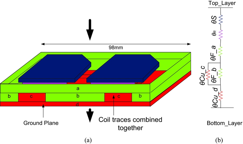
The simplified model is obtained by merging different sub-sections of the panel with the same material. The copper traces of different layers are merged into a single trace; similarly, FR4 material of the whole panel is also combined together. As a result, the FR4 and copper reduces to four sub-sections (a, b, c and d), as shown in Fig. 5(a). Sub-sections “a” and “b” have FR4 material while sub-sections “c” and “d” have copper. The parallel combination of the two solar cell resistors is represented by a single thermal resistance (θS ) and the associated resin resistors are also represented by a single thermal resistance (θR ). The modelling representation is identical to the previous one. Thermal model of Fig. 5(b) is written in mathematical form as given in Equation (5).
 $$\begin{equation}
{\theta _{th - S1S2}} = {\theta _S} + {\theta _R} + {\theta _{F\_a}} + {\theta _{Cu\_c}}//{\theta _{F\_b}} + {\theta _{Cu\_d}}
\end{equation}$$
(a) Panel top-to-bottom cross-sectional view and (b) panel simplified model.
3.1.2 Edge-to-edge thermal model of the CubeSat panel
Thermal resistance between the two sides “B” and “D” of the panel also called edge-to-edge thermal resistance (ϴth_BD or ϴEE), as shown in Fig. 3, is found using the proposed detailed and simplified thermal models discussed in the subsequent sections.
3.1.2.1 Detailed thermal model
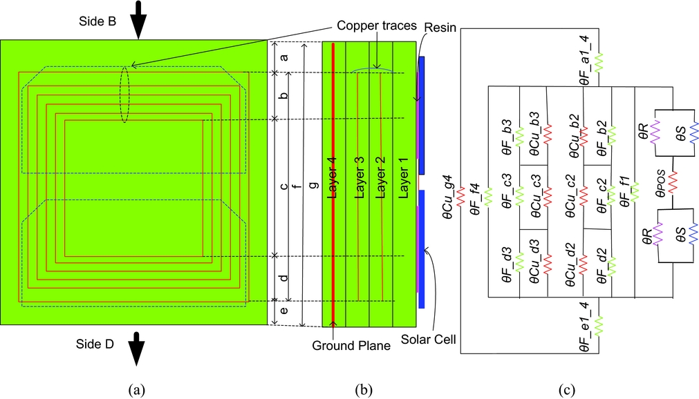
The panel has been divided into small sub-sections of different lengths with respect to the type of material as shown in Fig. 6. The sub-sections “a” and “e” have pure FR4 material in layers 1, 2, and 3 while the ground plane is embedded in layer 4. Similarly the sub-sections “b, c and d” consist of both FR4 and copper traces. In sub-sections “b” and “d,” the individual resistance of the copper traces is in series with each other while in sub-section “c,” copper traces resistance is in parallel with each other. Sub-section “f” has the FR4 material of layers 1 and 4, while sub-section “g” has the ground plane. The thermal model is obtained by combining the thermal resistance associated with each sub-section. The solar panel internal view, side view and edge-to-edge detailed thermal model are shown in Fig. 6.
Panel (a) internal view (b) side view (c) detailed thermal model.
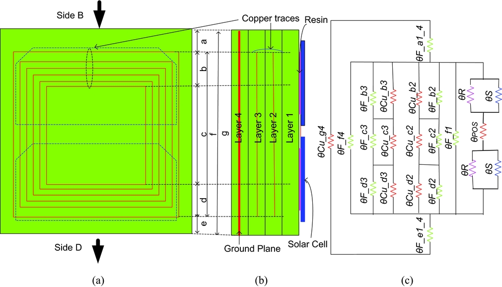
The thermal model of Fig. 6(c) is written in mathematical form as given in Equation (6) where “I” represents the number of layers that have copper traces and “j” represents the number of ground planes.
 $$\begin{equation}
\begin{array}{@{}l@{}} {\theta _{th - BD}} = {\theta _{EE}} = (2({\theta _R}//{\theta _S}) + {\theta _{POS}})//\left( {\frac{{{\theta _{F\_b}}//{\theta _{Cu\_b}} + {\theta _{F\_c}}//{\theta _{Cu\_c}} + {\theta _{F\_d}}//{\theta _{Cu\_d}}}}{i}} \right)\\ //{\theta _{F\_f1}}//{\theta _{F\_f4}} + {\theta _{F\_a1\_4}} + {\theta _{F\_e1\_4}})//\frac{{{\theta _{Cu\_g4}}}}{j} \end{array}
\end{equation}$$
3.1.2.2 Simplified model
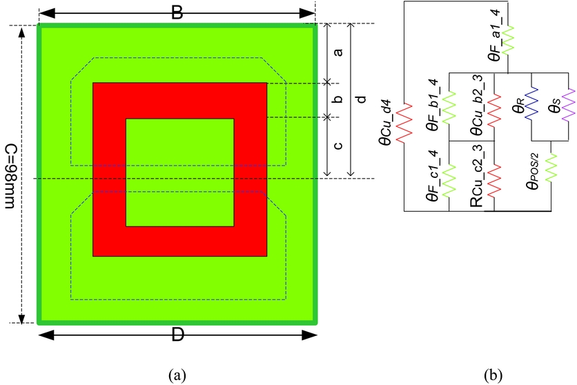
The detailed model from edge to edge of the panel is very complicated and requires complex computations of resistors as it is apparent from Fig. 6(c). Through a simplified model, the complex system is made simpler by combining different sub-sections of the panel having similar material. The copper traces in different layers are merged into a single trace. Similarly, the FR4 material is also shifted and combined.
The equivalent thermal model for the half portion of the panel is shown in Fig. 7(b), the other half being identical. Sub-section “a” has pure FR4 material, while sub-sections “b” and “c” consist of copper traces and FR4 material.
(a) Panel shape after combining similar material; (b) Panel half portion simplified model.
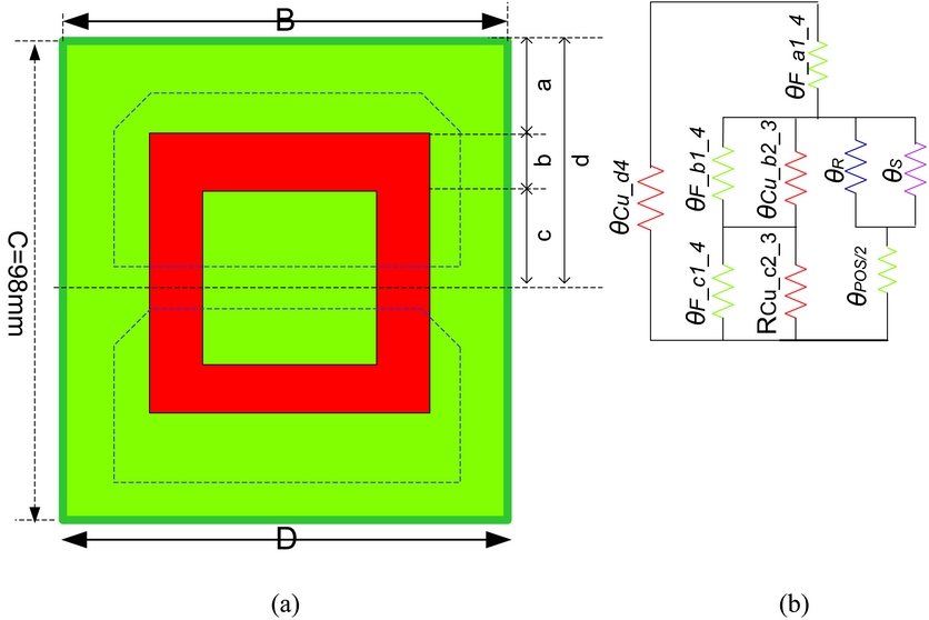
The simplified thermal model of a complete panel shown in Fig. 7 is given in Equation (7).
 $$\begin{equation}
\begin{array}{@{}l@{}} {\theta _{th - BD}} = {\theta _{EE}} = 2[({\theta _{F\_a1\_4}} + ({\theta _{F\_b1\_4}}//{\theta _{Cu\_b2\_3}} + {\theta _{F\_c1\_4}}//{\theta _{Cu\_c2\_3}})\\ //({\theta _s}//{\theta _R} + \frac{{{\theta _{POS}}}}{2}))//{\theta _{Cu\_d4}}] \end{array}
\end{equation}$$
3.1.3 Centre-to-edge thermal model of the CubeSat panel
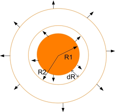
The centre-to-edge thermal model is based on the thermal resistance between two circles as shown in Fig. 8. The solar power is impinging on the circle with radius R1 and spreads to the circle with radius R2.
Thermal resistance between two circles.
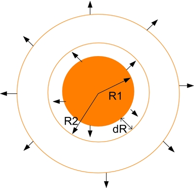
The solar power (P) absorbed by the circle with radius R is given by Equation (8);
 $$\begin{equation}
P = {P_d}\alpha \pi {R^2},
\end{equation}$$
where “Pd” is the solar power density and “α” is the absorption coefficient of the circle with radius R.
The temperature difference (ΔT) of the length dR is given by Equation (9).
 $$\begin{equation}
\begin{array}{@{}l@{}} dT = Pd\theta \\ dT = P\frac{{dR}}{{K2\pi R.h}}\\ dT = {P_d}\alpha \pi {R^2}\frac{{dR}}{{K2\pi R.h}} = \frac{{{P_d}\alpha }}{{2Kh}}RdR\\ \int\limits_{{R_1}}^{{R_2}} {dT} = \frac{{{P_d}\alpha }}{{2{P_d}Kh}}\int\limits_{{R_1}}^{{R_2}} {RdR} = \frac{{\alpha ({R_2}^2 - {R_1}^2)}}{{4K \cdot h}}\\ \Delta T = \frac{{\alpha {P_d}}}{{4Kh}}({R_2}^2 - {R_1}^2) \end{array}
\end{equation}$$
Here, “K” is the thermal conductivity of the material and “h” is the thickness of the circular section.
Thermal resistance of the section with length dR, as shown in Fig. 8, is given by Equation (10).
 $$\begin{equation}
\begin{array}{@{}l@{}} \Delta \theta = \frac{{\Delta T}}{P}\\ \Delta \theta = \frac{{\frac{{\alpha {P_d}{R_T}^2}}{{4Kh}}}}{{{P_d} \cdot \pi \cdot {R_T}^2}} = \frac{\alpha }{{4\pi Kh}} \end{array}
\end{equation}$$
Therefore, the thermal resistance of a circular section depends on the thickness of that section and the material absorption coefficient (α).
3.1.3.1 Detailed thermal model
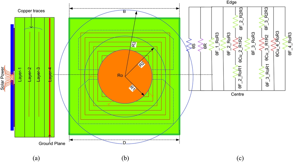
Assume the panel consists of three concentric circles with radius R1, R2 and R3, respectively, with centre R0 as shown in Fig. 9. The section between the radii R1 and R0 contains FR4 material and also ground plane (extended in layer 4). The sub-section between circle R1 and R2 contains copper traces, FR4 material, and ground plane. The sub-section between circles R2 and R3 contains FR4 material and ground plane. The centre-to-edge detailed thermal model is shown in Fig. 9(c). Here RiRj (i, j = 0, 1, 2, 3) represents the sub-sections amongst four circles. For example, θF_2_R1R2 represents the thermal resistance of FR4 material in layer 2 of the sub-section between circles R1 and R2. The rest of the modelling representation is identical to the previous models.
Panel (a) side view (b) internal view (c) detailed model.
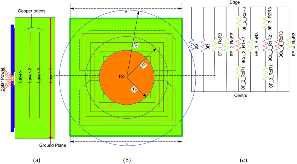
The thermal model of Fig. 9(c) is written in mathematical form as given in Equation (11).
 $$\begin{equation}
\begin{array}{@{}l@{}} {\theta _{th\_CE}} = {\theta _S}//{\theta _R}//{\theta _{F\_1\_{R_0}{R_3}}}//{\theta _{F\_2\_{R_0}{R_3}}}//({\theta _{F\_2\_{R_0}{R_1}}}\\ \qquad\qquad+\, {\theta _{Cu\_2\_{R_1}{R_2}}} + {\theta _{F\_2\_{R_2}{R_3}}})//{\theta _{F\_3\_{R_0}{R_1}}}//({\theta _{F\_3\_{R_0}{R_1}}}\\ \qquad\qquad+\, {\theta _{Cu\_3\_{R_1}{R_2}}} + {\theta _{F\_3\_{R_2}{R_3}}})//{\theta _{Cu\_4\_{R_0}{R_3}}}//{\theta _{F\_4\_{R_0}{R_3}}} \end{array}
\end{equation}$$
3.1.3.2 Simplified thermal model
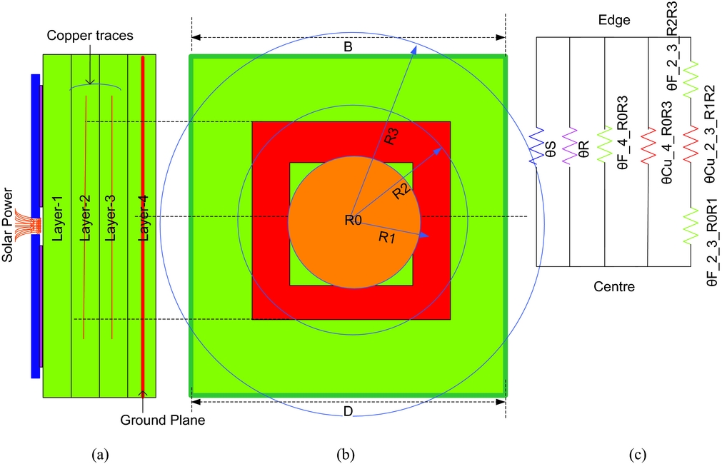
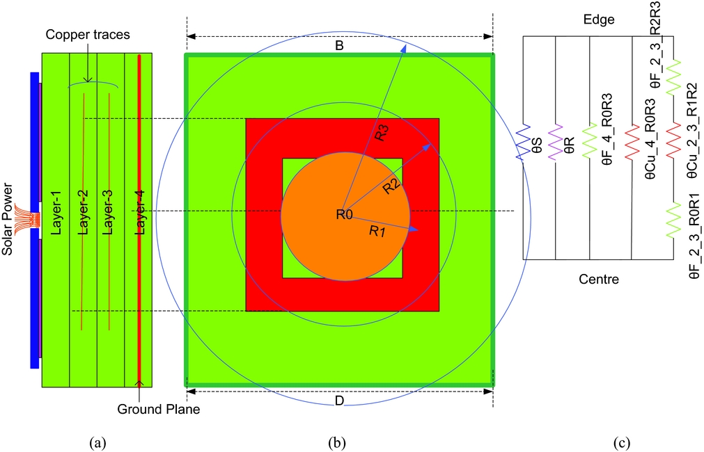
The centre-to-edge simplified thermal model is given in Fig. 10(c) which is written in mathematical form as given in Equation (12). The thermal modelling representation is identical to the previous models.
 $$\begin{equation}
\begin{array}{@{}l@{}} {\theta _{th - CE}} = {\theta _S}//{\theta _R}//{\theta _{F\_4\_{R_0}{R_3}}}//{\theta _{Cu\_4\_{R_0}{R_3}}}\\ //({\theta _{F\_2\_3\_{R_0}{R_1}}} + {\theta _{Cu\_2\_3\_{R_1}{R_2}}} + {\theta _{F\_2\_3\_{R_2}{R_3}}}) \end{array}
\end{equation}$$
Panel (a) side view (b) internal view (c) simplified model.
3.2 CubeSat thermal model
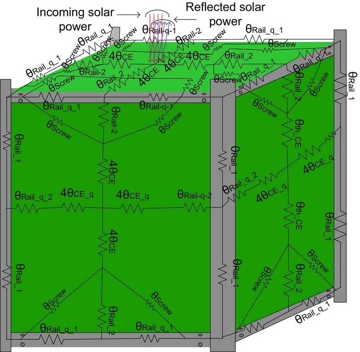
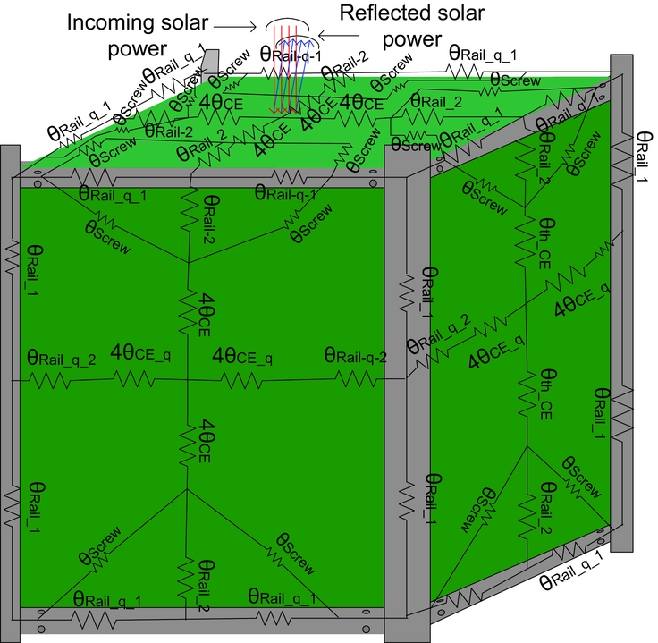
In the CubeSat thermal model, we are interested to measure the thermal resistance of the CubeSat from the centre of the top panel to the centre of the bottom panel. To develop this model, either the centre-to-edge thermal resistance model (θCE) or the edge-to-edge thermal resistance model (θEE) of the CubeSat panel can be used. When two θCE are added in series results in equivalent θEE. Here, θCE is used to develop the CubeSat thermal model shown in Figs. 11–13.
CubeSat with thermal resistances.
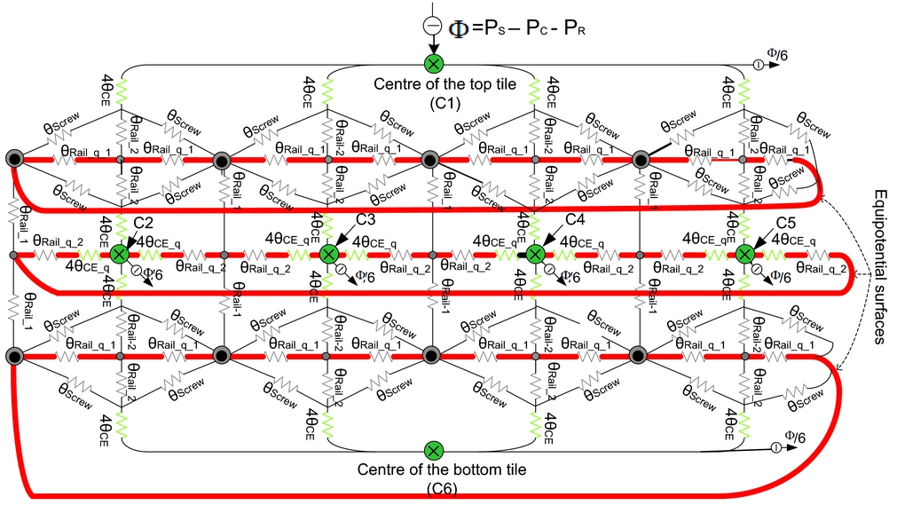
CubeSat thermal model along with equi-potential surfaces resistors.

CubeSat thermal model without equi-potential surface resistors.
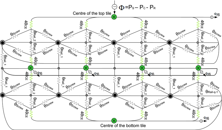
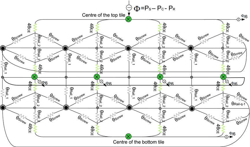
In the CubeSat thermal modelling, it is assumed that solar power ‘ϕ’ is impinging on the panel centre on one face of the satellite and equally spread out (ϕ/6 to each panel) to the coolest point on the opposite face of the satellite. Each panel, rail and screw has an associated thermal resistance. θCE is divided into four parallel resistances, each of 4θCE which is connected with lateral rails either direct or through screws. 4θCE is in series with the parallel combination of two screw resistance (θScrew) and one lateral rail resistance (θRail_2). θRail-1-q is the aluminum rail-to-rail thermal resistance on equi-potential surface (represented with a bold line in Fig. 12). At this point, thermal modelling of the top tile is completed. After this, the middle four tiles and the bottom tile have their thermal resistances. In their thermal models, the centre of each tile is represented by a circle with a cross (×), i.e. six tiles have six centres represented with letters C1 to C6. The corners of the satellite are represented by a circle with a dot (●). The centre of the rails is represented with a small circle as shown in Fig. 13. Each tile has 4θCE resistance from the centre to the rail. The next tile is connected with the previous one through rails, and screws have resistances θRail_2 and θScrew, respectively, and their parallel combination is connected in series with 4θCE. The surfaces on the CubeSat thermal model at the same temperature level are termed as equi-potential surfaces. The resistors on the equi-potential surfaces are represented with sub-script “q”. The temperature difference across the equi-potential surfaces resistance is zero; therefore, these resistors do not contribute to the thermal model and can be omitted from the CubeSat thermal model. The CubeSat thermal model without equi-potential thermal resistances is shown in Fig. 13.
The only power source of the CubeSat is the six solar panels covering as many faces of the satellite. By taking into account that only one panel is exposed at a time to sunlight, here are two cases where the power absorbed by the panel may be different. When the solar panel is on, it absorbs some portion of the incoming solar power (PS ) and the remaining power is reflected (PR ) from the surface. The amount of absorbed power depends on the absorption coefficient (α) of the exposed surface. Some portion of the absorbed power is converted to useful power (PC ), which depends on the efficiency (η) of the solar panel. The remaining absorbed power is transmitted to the satellite, which is the unwanted power (Φ), as given by Equation (13).
 $$\begin{equation}
\begin{array}{@{}*{1}{c}@{}} {\Phi = {P_S} - {P_R} - {P_C}}\\ { \Rightarrow \Phi = \alpha {P_d}S\left( {1 - \eta } \right)} \end{array}\quad \begin{array}{@{}*{1}{c}@{}} {\because {P_S} - {P_R} = \alpha {P_d}S\quad \quad \quad \quad }\\ {\& {P_C} = \eta \left( {{P_S} - {P_R}} \right) = \eta \alpha {P_d}S} \end{array}
\end{equation}$$
Here, Pd is the solar power density at Low Earth Orbit (LEO) is about 1,366 W/m2 and S is the area of the exposed surface.
When the solar panel is off, no power is converted to useful power and all the radiating power is transferred to the satellite.
 $$\begin{equation}
\Phi = \alpha {P_d}S
\end{equation}$$
The unwanted power (Φ) starts flowing to the coolest point on the satellite which is the centre point on the opposite face, as shown in Fig. 13. This power tends to increase the overall temperature of the satellite. The unwanted power (Φ) flows to all the six faces and is equally distributed amongst them (Φ/6 to each face).
The thermal model of Fig. 13 can be written in mathematical form as given in Equation (15). The symbol abbreviations used in Equation (15) are given in Table 2.
 $$\begin{equation}
{\theta _{th}} = 2\left( {\frac{{4{\theta _{CE}} + {\theta _{{\rm{Rail\_}}2}}//\frac{{{\theta _{{\rm{Screw}}}}}}{2}}}{4}} \right) + 2{\left( {\frac{4}{{4{\theta _{CE}} + {\theta _{{\rm{Rail}} - 2}}//\frac{{{\theta _{{\rm{Screw}}}}}}{2}}} + \frac{4}{{{\theta _{{\rm{Rail}}\_1}}}}} \right)^{ - 1}}
\end{equation}$$
4.0 THERMAL MODEL APPLICATION ON CUBESAT STANDARD NANOSATELLITE ARAMIS-C1
4.1 Thermal resistance of the AraMiS-C1 panels
As already mentioned, four sides of the AraMiS-C1 are equipped with four identical CubePMT and the remaining two sides have CubeSat Tele-Communication Tiles (CubeTCT). In order to find the thermal resistance of AraMiS-C1, it is first required to find the thermal resistances of the CubePMT and CubeTCT. The thermal models presented for the CubeSat panel in the previous section are applied to the CubePMT and CubeTCT and their thermal resistances are measured.
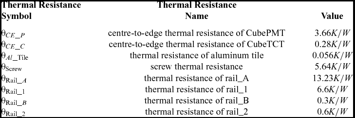
The CubePMT module has an almost identical structure with the CubeSat panel with just increased number of layers, copper traces and ground planes. Changing the number of layers and traces will modify the dimensions of the respective sub-sections which will result in different thermal resistance values for the CubePMT as compared to CubeSat panel. The thermal resistance model will remain the same as that of the CubeSat's panel. The CubePMT top-to-bottom and centre-to-edge thermal resistances have been measured by applying the CubeSat panel top-to-bottom and centre-to-edge detailed and simplified thermal models presented in the previous sections. The values for these resistances are given in Table 1.
Thermal resistances for the AraMiS-C1 thermal model theoretical measurements

4.2 Thermal resistance of AraMiS-C1 utilising the CubeSat model
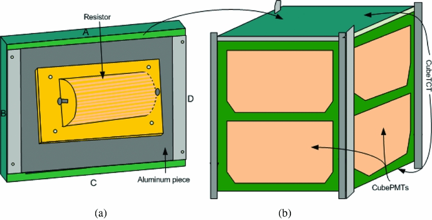
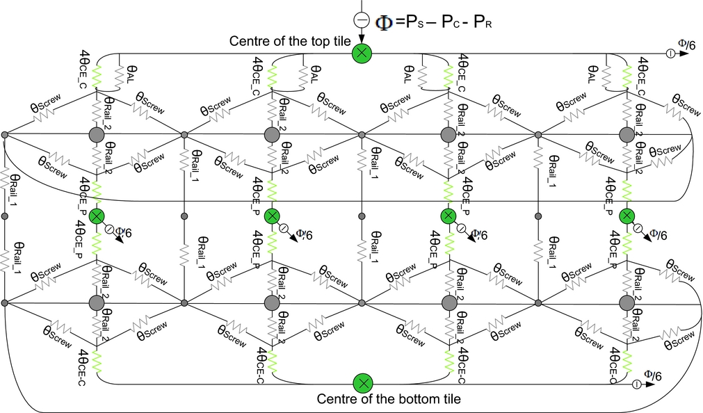
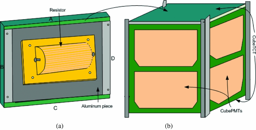
The CubeSat model presented in the previous section is used to measure the thermal resistance of AraMiS-C1. This theoretical measured resistance is then verified through a lab experimental set-up explained in the next section. For practical measurement of the equivalent thermal resistance of AraMiS-C1, a heat source is required to supply thermal power to the satellite comparable to the incoming solar power. For this purpose, a solar simulator can be used; but these measurements were performed inside a vacuum chamber. In that case, it is impossible to take the solar simulator inside the vacuum chamber. For this purpose, a 2.2 Ω and 100 W resistor is used that can raise the satellite one face temperature equivalent to the temperature increase by the sunlight at AM0. This resistor was attached with the CubeTCT through an aluminum piece as shown in Fig. 14. Due to the addition of an aluminum piece, a little modification is made in the CubeSat thermal model shown in Fig. 13. A thermal resistance in the form of an aluminum piece (θAl) has been added in parallel with the top tile, and the thermal resistance from centre-to-edge (θCE) has been modified with (θCE_C) and (θCE_P), which represent CubeTCT centre-to-edge thermal resistance and CubePMT centre-to-edge thermal resistance, respectively, as shown in Fig. 15.
Measurement arrangements of AraMiS-C1. (a) Power resistor attached with CubeTCT through aluminum tile. (b) AraMiS-C1 with four CubePMT without solar cells and two CubeTCT tiles.
Equivalent thermal model of the AraMiS-C1 measurement arrangement.
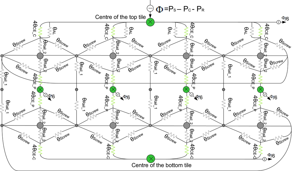
The equivalent thermal model of the AraMiS-C1 satellite with the measurement arrangement is shown in Fig. 15.
 $$\begin{eqnarray}
{\theta _{th}} &=& \left( {\frac{{4{\theta _{CE\_C}}//4{\theta _{Al}} + {\theta _{{\rm{Rail}}\_2}}//\frac{{{\theta _{{\rm{Screw}}}}}}{2}}}{4}} \right) + \left( {\frac{{4{\theta _{CE\_C}} + {\theta _{{\rm{Rail}}\_2}}//\frac{{{\theta _{{\rm{Screw}}}}}}{2}}}{4}} \right)\nonumber\\
&& +\, 2{\left( {\frac{4}{{4{\theta _{CE\_P}} + {\theta _{{\rm{Rail}}\_2}}//\frac{{{\theta _{{\rm{Screw}}}}}}{2}}} + \frac{4}{{{\theta _{{\rm{Rail}}\_1}}}}} \right)^{ - 1}}
\end{eqnarray}$$
The thermal model of Fig. 15 is mathematically expressed in Equation (16). This model is identical to that of the CubeSat thermal model except the aluminum resistor is in parallel with the CubeTCT tile. In the CubeSat model, there is CubePMT thermal resistance instead of CubeTCT and aluminum thermal resistances parallel combination.
In thermal measurements, the CubePMT was without solar cells and resins. Therefore, these two resistors were omitted in the theoretical measurements. All the required resistors for the AraMiS-C1 thermal model theoretical measurements are given in Table 1.
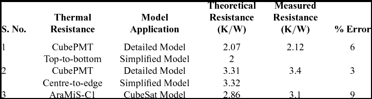
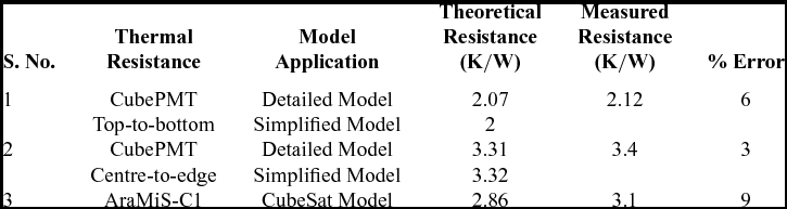
Inserting all the required resistors values in Equation (16), the equivalent thermal resistance of AraMiS-C1 found is 2.86 K/W.
5.0 THERMAL MODEL VERIFICATION THROUGH LABORATORY EXPERIMENTS
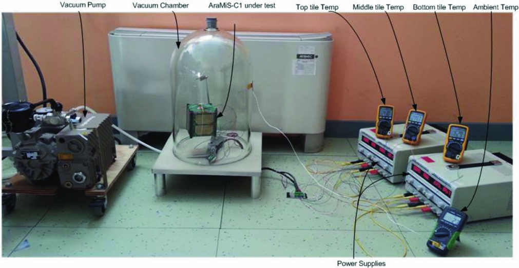
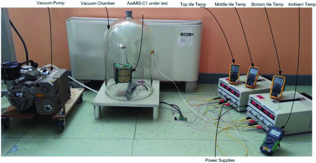
In the previous section, the theoretical thermal resistance value of AraMiS-C1 is found using the thermal model presented for the CubeSat standard nanosatellite. In order to verify the theoretical results, the practical value of the AraMiS-C1 thermal resistance was found using the experimental set-up shown in Fig. 16. The set-up is composed of AraMiS-C1 with measurement arrangements, temperature sensors, a data acquisition system, vacuum chamber and vacuum pump. A power resistor is attached to the CubeTCT in order to provide power to the top tile of AraMiS-C1 equivalent to the solar power provided by the AM0 intensity light in LEO.
AraMiS-C1 thermal resistance measurement experimental set-up.
In order to find thermal resistance, power absorbed and corresponding temperature difference values are required. For the AraMiS-C1 thermal resistance measurement, a constant power will be provided to one side of the satellite and the corresponding temperature difference between the tile where power is provided and the opposite side of the satellite will be measured, inside a vacuum chamber. Power applied and the resultant temperature difference will be recorded, and the resultant thermal resistance of AraMiS-C1 will be measured using Equation (3). For the AraMiS-C1 solar panel exposed to the sun with an area of 0.008085 m2 (98 mm×82.5 mm) and power density in LEO at AM0 is 1,365 W/m2, the power absorbed by AraMiS-C1 is 11W (1,365 W/m2×0.008085 m2).
In order to provide 11W power to AraMiS-C1, a laboratory set-up is used as shown in Fig. 16. Constant current of 5A is drawn through a 2.2 Ω power resistor. Three temperature sensors are attached to the top and bottom CubeTCT tiles and the side CubePMT tile of AraMiS-C1. Power supplies provide power to the temperature sensors and power resistor. A data acquisition system acquires data from the sensors.
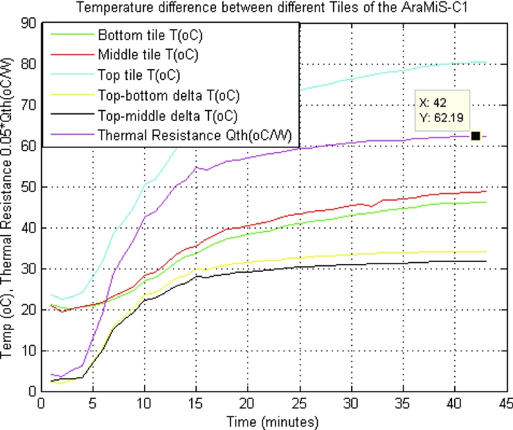
AraMiS-C1 is placed inside the vacuum chamber. After generating a vacuum inside the chamber, a constant current of 5A was drawn through the power resistor. The top CubeTCT tile started heating up and temperature sensors values started increasing. After some time, the temperature of tiles attained the steady state values, and data from the temperature sensors became stable. All the sensors’ data was acquired and continuously recorded during the experiment.
Figure 17 shows temperatures of top, middle and bottom tiles and their temperature differences. It also shows thermal resistance between top and bottom tiles, which is 3.1 K/W.
Thermal resistance and temperature difference between different faces of AraMiS-C1 satellite.
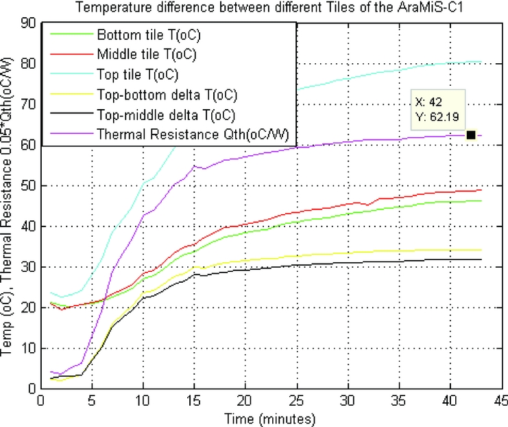
The thermal resistance of AraMiS-C1, found through the CubeSat mathematical model and experimental set-up, has almost the same value.
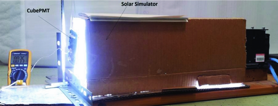
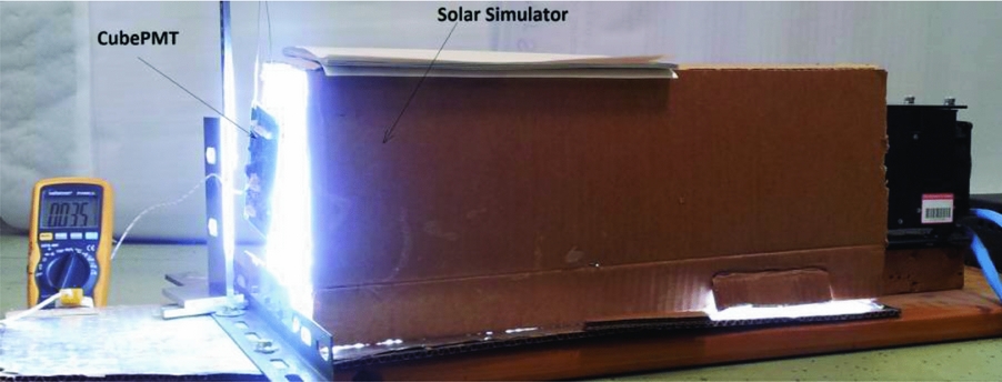
Practical resistance of CubePMT and CubeTCT modules are measured through the experimental set-up shown in Fig. 18. Table 2 shows that there is very little difference between the theoretical and measured values, which reflects the authenticity of the proposed models.
CubePMT thermal resistance measurement experimental set-up.
Thermal model application and measurement results
6.0 SOLAR POWER ABSORBED AND TEMPERATURE DIFFERENCE
The only power source of AraMiS-C1 are the six solar panels covering as many faces of the satellite. Each solar panel with two solar cells has an area of about 2×70×40 mm2. Sun power density at LEO is about 1366 W/m2. When one panel is exposed at a time to sunlight, there are two cases where the power absorbed by the CubePMT single module will be different.
-
• When the solar panel is on, it absorbs 26% of power and remaining 74% power is lost through the CubePMT module. The power absorbed by the AraMiS-C1 is 5.1 W.
-
• When solar panel is off, all the radiating power is transferred to the CubePMT module. The absorption area (A) is the CubePMT surface area (98×82.5 mm2) and solar cell efficiency (η) will become zero in Equation (2). The power absorbed by the AraMiS-C1 is 11 W.
In order to find the temperature difference (ΔT) between different points of a spacecraft, thermal resistance and solar power absorbed are required as given in Equation (3).
The temperature difference (ΔT) between various sides of the CubePMT module can be found using Equation (3) in two different cases:
-
• When the solar panel is on: ΔT from the top-to-bottom layer of the CubePMT is (5.1 W × 2 K/W) 10.2 K, while from centre-to-edge, the ΔT is (5.1 W × 3.2 K/W) 16.3 K.
-
• When the solar panel is off: ΔT from the top-to-bottom layer of the CubePMT is (11 W×2 K/W) 22 K, while from centre-to-edge, the ΔT is (11 W×3.2 K/W) 35.2 K.
In case of AraMiS-C1, it is assumed that power is absorbed through a single CubePMT module perpendicular to the incoming solar radiations. All the other tiles are in the dark. The temperature difference (ΔT) from top-to-bottom of AraMiS-C1 using Equation (3) can be found in two different cases:
-
• In the case when the solar panel is on: ΔT value is (5.1 W × 3 K/W) 15.3 K.
-
• When the solar panel is off: ΔT value is (11 W × 3 K/W) 33 K.
7.0 CONCLUSION
In this paper, thermal models have been presented for the CubeSat compatible panels and spacecrafts. The detailed and simplified models proposed for a single panel were presented. The corresponding models were applied to the AraMiS-C1 panels (CubePMT) and the thermal resistance values were found. The difference between the resistance values measured through both models is low that verifies the verification of the proposed models.
The thermal resistance of the whole system was found by employing the presented CubeSat thermal model. In order to verify the value of the thermal resistance measured through the CubeSat model, the AraMiS-C1 thermal resistance was measured through an experimental set-up. The minimum deviation of the theoretical and experimental results indicates the verification of the model presented for CubeSat. In conclusion, the presented models are reliable and can be applied to any CubeSat standard nanosatellites. The calculated and measured thermal resistance values of our test spacecraft are very low which qualifies the thermal design of our test spacecraft. The low thermal resistance ensures that the spacecraft can easily dissipate heat from a hotter to a cooler surface.
The amount of power absorbed by the CubePMT module and AraMiS-C1 satellite under different conditions is calculated. Temperature differences between different points of the single tile and complete satellite were measured.
The presented models and measurement techniques can be used for the measurement of thermal resistance, power absorption and temperature difference between different points of the CubeSat standard nanosatellites.