1 Introduction
The density-driven spreading of immiscible fluids within a horizontal porous medium is a rich problem with applications to the modelling of groundwater flows, contaminant spills (non-aqueous phase liquids) and the long-term storage of carbon dioxide (
 $\text{CO}_{2}$
) in saline aquifers. Multiphase gravity currents containing a finite volume of fluid are particularly challenging to model due to hysteresis in the behaviour of capillary forces between advancing and receding fronts. Yet it is the macroscopic manifestation of hysteresis between fluids and solids in contact at the pore scale that ultimately results in fluid being permanently trapped within a porous media. These processes, which act to trap some fraction of the mobile fluid within the confines of the small pore space, have large consequences, dictating the distance over which fluid may migrate under buoyancy forces. For example, in geological carbon storage an accurate determination of the distance a volume of
 $\text{CO}_{2}$
input may travel is critical to the deployment of this technology.
There are three primary manifestations of two-phase flow. Firstly, the interaction between two immiscible fluids as one displaces the other, along with the geometry of the porous medium, causes an uneven distribution of fluid saturation. The saturation is determined by capillary pressure, which is set by the hydrostatic gravitational pressure gradient in a gravity current, as discussed in detail below. Secondly, variations in the partial saturation lead to differences in the relative permeability of each fluid in the current, which affect its overall dynamics. Finally, hysteresis in the action of capillary forces when one immiscible fluid displaces another leads to trapping of the displaced fluid. Trapping of the non-wetting fluid in the form of isolated ganglia, or bubbles, is known as residual trapping. It is well established that the saturation of residually trapped, non-wetting fluid depends on the historical saturation distribution and therefore needs to be described by an empirical trapping model (Land Reference Land1968; Pentland et al. Reference Pentland, Al-Mansoori, Iglauer, Bijeljic and Blunt2008).
The spreading and residual trapping of a finite volume of fluid was first investigated by Kochina, Mikhailov & Filinov (Reference Kochina, Mikhailov and Filinov1983), who considered a slumping groundwater mound. As the mound slumps, wetting fluid is left behind and the saturation of residually trapped fluid, as well as in the spreading current, is assumed to be constant and uniform. Kochina et al. (Reference Kochina, Mikhailov and Filinov1983) found that the evolving height profile is described by a similarity solution of the second kind in which the power-law spreading rate must be solved numerically and is a function only of the ratio of trapped to initial fluid saturation. The mound spreads ever more slowly as an increasing proportion of fluid is residually trapped. The initial conditions, such as the horizontal extent and volume, affect the time scale on which the current spreads but not the power-law exponent of spreading. Uniform saturation models have also been applied to the geological storage of
 $\text{CO}_{2}$
, where a constant saturation of fluid is assumed in both mobile and trapped regions (Bear et al.
Reference Bear, Ryzhik, Braester and Entov1996; MacMinn & Juanes Reference MacMinn and Juanes2009; Juanes, MacMinn & Szulczewski Reference Juanes, MacMinn and Szulczewski2010). These models assume that capillary effects on the dynamics of the gravity current are negligible, although some attempts have been made to capture the hysteresis inherent in two-phase flow (Gasda, Nordbotten & Celia Reference Gasda, Nordbotten and Celia2009). More recent studies have shown that, particularly for monodisperse media, capillary hysteresis can ultimately lead to blunting and pinning of immiscible gravity currents (Zhao et al.
Reference Zhao, Macminn, Szulczewski, Neufeld, Huppert and Juanes2013, Reference Zhao, Macminn, Huppert and Juanes2014).
Multiphase models that resolve the saturation distribution within two-phase currents were originally developed for applications to groundwater hydrology and petroleum engineering (Parker & Lenhard Reference Parker and Lenhard1989; Bear et al.
Reference Bear, Ryzhik, Braester and Entov1996). They enable the use of constitutive relations linking capillary pressure and relative permeability to saturation. Recently, variable saturation models have been applied to the injection stage of the geological storage of
 $\text{CO}_{2}$
(Golding et al.
Reference Golding, Neufeld, Hesse and Huppert2011; Nordbotten & Dahle Reference Nordbotten and Dahle2011; Golding, Huppert & Neufeld Reference Golding, Huppert and Neufeld2013). Golding et al. (Reference Golding, Neufeld, Hesse and Huppert2011) investigated how the spatial sweep of steady-state, constant-flux gravity currents is affected by the properties of the porous medium and the relative strength of capillary and gravitational forces. Golding et al. (Reference Golding, Huppert and Neufeld2013) demonstrated that the time-dependent propagation of an axisymmetric gravity current, fed by a constant flux, can be described by a similarity solution, spreading like
 $t^{1/2}$
, similar to comparable currents containing only a single phase (for example miscible currents which we refer to as single-phase currents throughout). The vertical integration of pore-scale effects in these multiphase models make numerical computations of gravity current predictions significantly faster, even when incorporating complex geological or empirical multiphase data.
Given its significant impact on the long-term security of geologically stored
 $\text{CO}_{2}$
, detailed consideration of residual trapping has received surprisingly little consideration. In previous studies, we suggested how estimates could be improved by applying a trapping model to the saturation profile of a current at the end of the injection phase (Golding et al.
Reference Golding, Neufeld, Hesse and Huppert2011, Reference Golding, Huppert and Neufeld2013). However, this does not predict the effect of trapped fluid on the dynamics of the current. Previously, Van Dijke & Van der Zee (Reference Van Dijke and Van der Zee1997) and Bear & Ryzhik (Reference Bear and Ryzhik1998) considered residual trapping of an oil lens at an air–water interface in the long-time limit. They introduced residual trapping into their models by relating residual trapping to the volume of fluid per unit area of the current, as an intermediate step towards incorporating a constitutive relationship between initial and residual saturation. In numerical simulations, in particular petroleum engineering, Land’s trapping model (Land Reference Land1968) has commonly been employed. Land’s nonlinear trapping model predicts that a higher proportion of fluid is trapped at low initial saturations than at high initial saturations of the non-wetting fluid. This might be explained by the non-wetting fluid being more easily isolated from the rest of the flow when it occupies the pore space at a low saturation. A more recent study by Doster, Nordbotten & Celia (Reference Doster, Nordbotten and Celia2013) discusses the incorporation of Land’s trapping model into variable saturation, or vertical equilibrium, models showing how trapping hysteresis may be incorporated into the formalism, but without exploring the consequences for propagation and ultimate trapping.
One of the central results of this paper is that the choice of trapping model is fundamental in determining the long-term behaviour of a finite-volume, two-phase gravity current. This means that the choice of trapping model is not trivial and predictions for the long-time spreading of the current should be interpreted carefully. In particular, and in contrast to the linear trapping relation, we argue that if the ratio of trapped to initial fluid saturation increases as saturation decreases, a gravity current will slow down at a faster rate. Furthermore, if the ratio tends to unity, as is the case for Land’s model, the results suggest that the gravity current will stop in finite time.
In this paper we develop an original analytical model for a two-phase gravity current resulting from the release of a finite volume of fluid. In § 2.1 we begin with a physical description of our model and how it differs from the classic model of Kochina et al. (Reference Kochina, Mikhailov and Filinov1983). The model captures the key two-phase phenomena in regions of drainage and imbibition, including hysteresis of capillary pressure and relative permeability, and the use of scanning curves during secondary imbibition. One of the key strengths of our framework is that it permits the use of any trapping relation, and we use this flexibility to discover the significant impact the trapping characteristics have on the long-time behaviour of the gravity current. Throughout § 2, we continue to develop the framework for a two-phase gravity current resulting from the release of a finite volume of fluid, where all capillary effects, including the saturation distribution and trapping, discussed in §§ 2.2 and 2.3, are conveniently and consistently included. The saturation and flux functions are independently defined in § 2.4 for each region. We describe our boundary conditions in § 2.5 and formulate the problem in terms of dimensionless variables in § 2.6, identifying the key dimensionless parameters which determine the behaviour of the gravity currents. We use the model to examine how the key factors affect the propagation rate and height profile of the spreading of non-wetting fluid in § 3. In the long-time limit, under certain conditions, the finite-volume two-phase gravity current spreads in a self-similar way as described by a similarity solution of the second kind, derived in § 3.1. More generally, numerical solution of the full equations using the linear model in § 3.2 verifies the self-similar spreading in the long-time limit, similar to the constant-saturation model by Kochina et al. (Reference Kochina, Mikhailov and Filinov1983). In striking contrast, numerical solution of the equations using Land’s model in § 3.3 leads to gravity currents whose spreading stops at a finite runout distance. Implications of our findings on the efficiency of residual trapping is discussed in § 4, where we discover that Land’s model predicts a greater efficiency of trapping within a smaller radial extent. Our conclusions are summarised in § 5 along with a discussion of the implications for the geological storage of
 $\text{CO}_{2}$
.
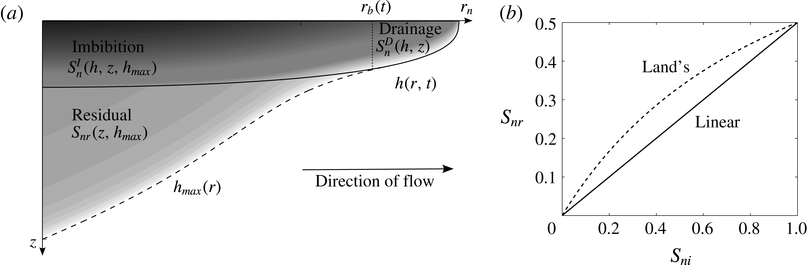
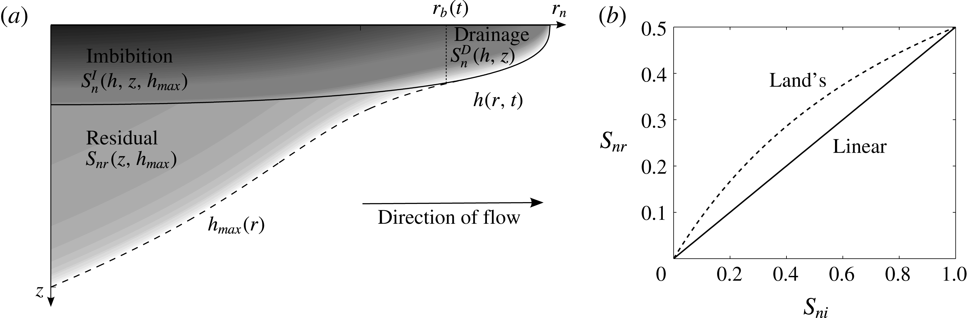
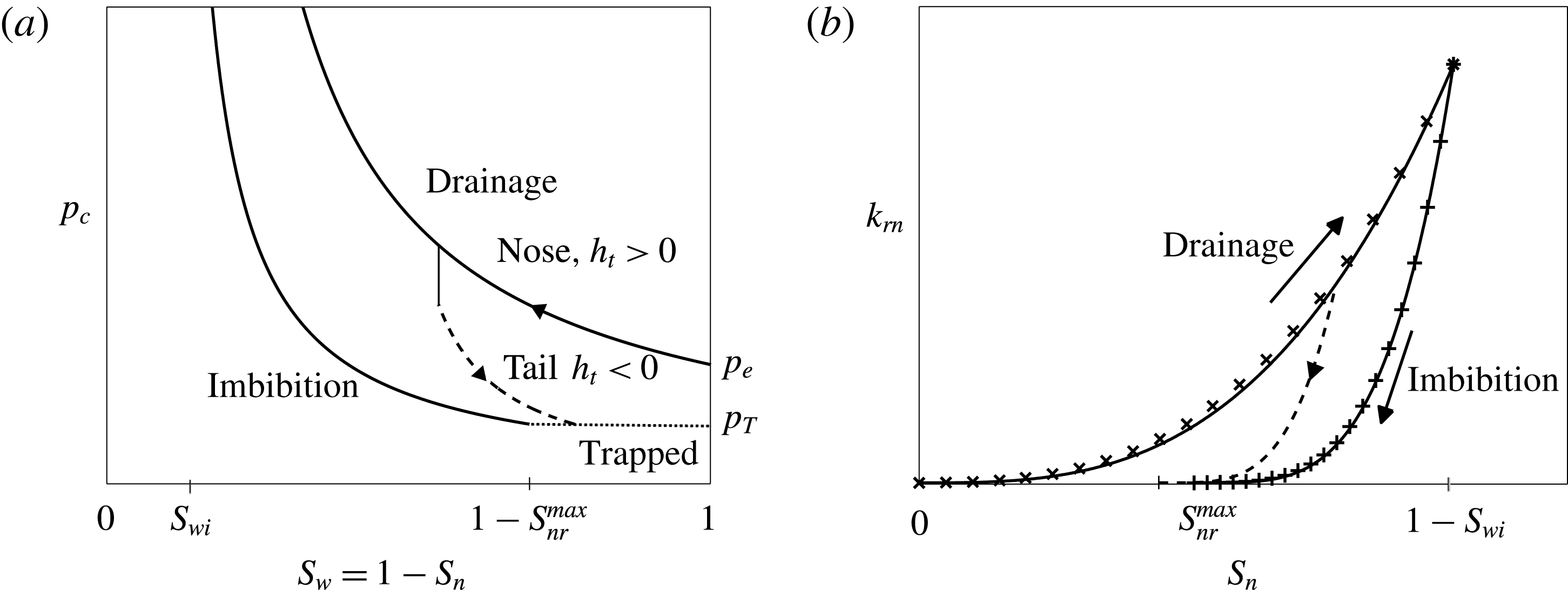
(a) Sketch of a two-phase gravity current resulting from a finite release of a non-wetting fluid into a porous medium initially saturated with denser, wetting fluid. The schematic shows the advancing drainage front, the receding imbibition front and the region of immobile, residually trapped fluid. The saturation distributions in the drainage and imbibition zones vary in space and time, while in the trapped region the distribution is spatially non-uniform although static. (b) Example of two trapping models, relating the residually trapped saturation,
 $S_{nr}$
, to the initial non-wetting phase saturation at the onset of drainage,
 $S_{ni}$
. Land’s model is a nonlinear relation, where almost all the fluid is trapped if drainage begins at a low saturation, in contrast to the linear model, where the same proportion of fluid is trapped at any stage.
2 Theory and model development
We consider the axisymmetric spreading and residual trapping of a finite volume of buoyant, non-wetting fluid in a porous medium of porosity
 $\unicode[STIX]{x1D719}$
and intrinsic permeability
 $k$
(see figure 1
a). The initial fluid configuration will, in general, be the end result of an injection phase during which we imagine a primary drainage process sets the initial, axisymmetric fluid distribution as a function of both the radial and vertical coordinates,
 $r$
and
 $z$
respectively. For high aspect ratio initial conditions, the pressure within the current is nearly hydrostatic, and so a balance between gravity and capillary forces, so-called gravity–capillary equilibrium, sets the initial, vertical ‘saturation distribution’. The full details of this initial injection phase, including detailed discussion of the saturation distribution, have been presented previously by Golding et al. (Reference Golding, Neufeld, Hesse and Huppert2011, Reference Golding, Huppert and Neufeld2013). Here we utilise the same starting framework as those earlier studies, but significantly extend the conceptual framework to understand the large-scale dynamical consequences of capillary, or residual, trapping at the pore scale and the consequent hysteresis within advancing and receding regions of the current.
The mobile fluid within the gravity current can be separated into two distinct regions, separated by a moving boundary at
 $r=r_{b}(t)$
. The front of the current (
 $r>r_{b}$
) is advancing, with height
 $h$
increasing with time
 $t$
, and is undergoing drainage of wetting fluid, for example water draining from the pore space as
 $\text{CO}_{2}$
is emplaced. Towards the middle of the current (
 $r<r_{b}$
), the height is falling, and the fluids are undergoing secondary imbibition where, for example, water is re-entering the pore space occupied by
 $\text{CO}_{2}$
. Where the current is retreating, the fluid in the region
 $h<z<h_{\mathit{max}}$
(
 $r<r_{b}$
) lies immobile and residually trapped (see figure 1
a).
The current spreads radially below a horizontal barrier of infinite extent in an unconfined aquifer, for which the depth of current
 $h\ll \unicode[STIX]{x1D707}_{a}H/\unicode[STIX]{x1D707}_{c}$
is much less than the depth of the aquifer
 $H$
, where
 $\unicode[STIX]{x1D707}_{a}$
is the viscosity of the ambient fluid (for example water) and
 $\unicode[STIX]{x1D707}_{c}$
is the viscosity of the injected fluid (for example
 $\text{CO}_{2}$
) (for details on the unconfined limit see Pegler, Huppert & Neufeld Reference Pegler, Huppert and Neufeld2014). In this limit there is negligible flow of wetting phase far below the current, and since we assume that this phase is simply connected everywhere in the domain we can deduce that there is no horizontal pressure gradient in the wetting phase. This means that flow of the wetting phase can be neglected both within the current and the surrounding aquifer, resulting in a significant simplification of the model. The physics of the buoyant gravity current shown in figure 1(a) is equivalent to that of a volume of denser, non-wetting fluid spreading above an impermeable boundary and so the theory may equally be applied to the propagation of buoyant
 $\text{CO}_{2}$
as well as the trapping of dense contaminant spills, for example.
2.1 Physical interpretation of the model
The model presented here draws together a number of empirical measurements for permeability and saturation in multiphase flows in porous media into a vertically integrated framework for gravity currents. In this section we describe the basic physical basis for our framework and outline the similarities and differences between our model, which resolves the spatial structure of saturation, and the classic model of Kochina et al. (Reference Kochina, Mikhailov and Filinov1983) for which the saturation is treated as uniform within the advancing and retreating portions of the current.
We begin with a brief introduction to multiphase flow in this paragraph, and refer the reader to Golding et al. (Reference Golding, Neufeld, Hesse and Huppert2011) for a more detailed description of the physical and mathematical basis for multiphase flow in porous media. When two immiscible fluids flow through the narrow confines of the available pore space, they each occupy only a fraction of the available pore volume. This fraction is the fluid saturation, and a distinction is typically made between the wetting phase (e.g. water) which is more attracted to the solid and the non-wetting phase (e.g.
 $\text{CO}_{2}$
). The interfacial tension acting between the fluids, averaged over many pore spaces, results in a macroscopic pressure difference commonly referred to as the capillary pressure. Empirical models, discussed in much greater detail below, then describe measured relationships between the saturation, the capillary pressure between phases and the relative resistance to flow of each phase through the partially saturated media, known as the relative permeability.
Much as the action of surface tension on contact lines of droplets leads to a hysteresis between advancing and receding contact angles, within the pore space the combined action of contact lines in the complex pore geometry leads to an observed hysteresis of the capillary pressure between advancing and receding fluid fronts, as outlined in § 2.2. Ultimately, this combination of hysteresis and geometry conspire to leave isolated droplets of the non-wetting fluid which as a result are effectively trapped or immobilised. In general, it is observed that the magnitude of trapping is a function of the initial saturation, as shown schematically for two representative profiles in figure 1(b) and as discussed more fully in § 2.3.
The key finding of this work is that if the relationship between the initial saturation of a multiphase current and the fraction of non-wetting fluid trapped is nonlinear then the current propagates out only to finite distance. This is important in the context of previous work which considered constant and uniform saturations within the advancing and receding portions of the current and a linear trapping model (Kochina et al. Reference Kochina, Mikhailov and Filinov1983), and which found that the current propagates in a self-similar manner for all times. This self-similar spreading is replicated if, in our own model, we assume a linear trapping model while resolving the distribution of saturation within the current. Thus in all cases, a linear relationship between initial saturation and trapping fraction results in a current which propagates indefinitely. In contrast, a nonlinear relationship, which is more representative of many experimental studies, displaying greater efficiency of trapping at lower saturations, results in a finite lateral extent. The spreading of such multiphase currents with nonlinear trapping is explored in § 3.
In the remainder of this section we outline the theory required to develop a two-phase framework for the height evolution and saturation distribution of a finite-volume current, highlighting how and where trapping and hysteresis are incorporated.
2.2 The saturation distribution
In this subsection, we derive the distinct saturation distributions in the two regions of the current using the assumption of gravity–capillary equilibrium to yield the pressure distribution, along with empirical models relating capillary pressure to saturation.
The long, thin aspect ratio of gravity currents indicates that the flow is mainly horizontal and that pressure is therefore nearly hydrostatic in the vertical. This permits the assumption of gravity–capillary equilibrium which resolves the saturation distribution of non-wetting fluid in the current,
 $S_{n}(r,t)$
. As in previous studies (Golding et al.
Reference Golding, Neufeld, Hesse and Huppert2011, Reference Golding, Huppert and Neufeld2013), we use constitutive laws to relate capillary pressure to saturation and again choose the Brooks–Corey framework (Brooks & Corey Reference Brooks and Corey1964) for the simplicity of the description. However, in this scenario we require empirical relationships for secondary imbibition as well as primary drainage.
In the advancing region of the current, the saturation increases according to the Brooks–Corey capillary pressure curve for primary drainage, given by
 $$\begin{eqnarray}p_{c}(s)=p_{e}(1-s)^{-1/\unicode[STIX]{x1D6EC}_{D}},\end{eqnarray}$$
where
 $\unicode[STIX]{x1D6EC}_{D}$
parameterises the pore-size distribution and
 $p_{e}$
is the capillary entry pressure of the porous medium. A narrower pore-size distribution, represented by a larger value of
 $\unicode[STIX]{x1D6EC}_{D}$
, results in weaker capillary forces. A larger capillary entry pressure, which the non-wetting fluid must overcome to displace wetting fluid from a pore, results in stronger capillary forces. A more detailed interpretation of these parameters is discussed in Golding et al. (Reference Golding, Huppert and Neufeld2013), below equation (5b). We have defined the normalised non-wetting phase saturation,
 $$\begin{eqnarray}s=S_{n}/(1-S_{wi}),\end{eqnarray}$$
in terms of the irreducible wetting phase saturation
 $S_{wi}$
. From now on, a lower case
 $s$
denotes a normalised non-wetting phase saturation. For example,
 $s_{r}^{\mathit{max}}=S_{nr}^{max}/(1-S_{wi})$
denotes the normalised maximum possible non-wetting residual saturation at the end of a primary imbibition process.
At the tail of the current, in the imbibition region, the saturation at any position decreases from its known maximum at the point of flow reversal, denoted by
 $s^{\prime }$
, along a secondary imbibition scanning curve to its ultimate residual saturation,
 $s_{r}(s^{\prime })$
. To capture such scanning curves, we employ a capillary pressure model adapted by Gerhard & Kueper (Reference Gerhard and Kueper2003) which is based on the Brooks–Corey framework. This uses just the primary drainage curve (2.1) and the primary imbibition curve given by
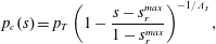 $$\begin{eqnarray}p_{c}(s)=p_{T}\left(1-\frac{s-s_{r}^{\mathit{max}}}{1-s_{r}^{\mathit{max}}}\right)^{-1/\unicode[STIX]{x1D6EC}_{I}},\end{eqnarray}$$
where
 $\unicode[STIX]{x1D6EC}_{I}$
is analogous to
 $\unicode[STIX]{x1D6EC}_{D}$
and
 $p_{T}<p_{e}$
is the terminal pressure defined to be the pressure at which non-wetting phase is immobile at its residual saturation. For ideal porous systems
 $\unicode[STIX]{x1D6EC}_{I}=\unicode[STIX]{x1D6EC}_{D}$
, because they both characterise the pore-size distribution. However, for more realistic porous media these parameters are estimated empirically, and so
 $\unicode[STIX]{x1D6EC}_{I}\neq \unicode[STIX]{x1D6EC}_{D}$
. Using these parameters, Gerhard & Kueper (Reference Gerhard and Kueper2003) defined capillary pressure scanning curves for imbibition after drainage (secondary imbibition) by
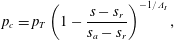 $$\begin{eqnarray}p_{c}=p_{T}\left(1-\frac{s-s_{r}}{s_{a}-s_{r}}\right)^{-1/\unicode[STIX]{x1D6EC}_{I}},\end{eqnarray}$$
where
 $s_{a}$
acts as an asymptotic saturation, akin to
 $1-S_{wi}$
in primary drainage. It is defined such that there is a discontinuous drop in capillary pressure equal to
 $p_{e}-p_{T}$
when the flow reverses at
 $s=s^{\prime }$
, reflecting the underlying physical hysteresis at the pore scale. This ensures that saturation remains continuous at the boundary
 $r=r_{b}$
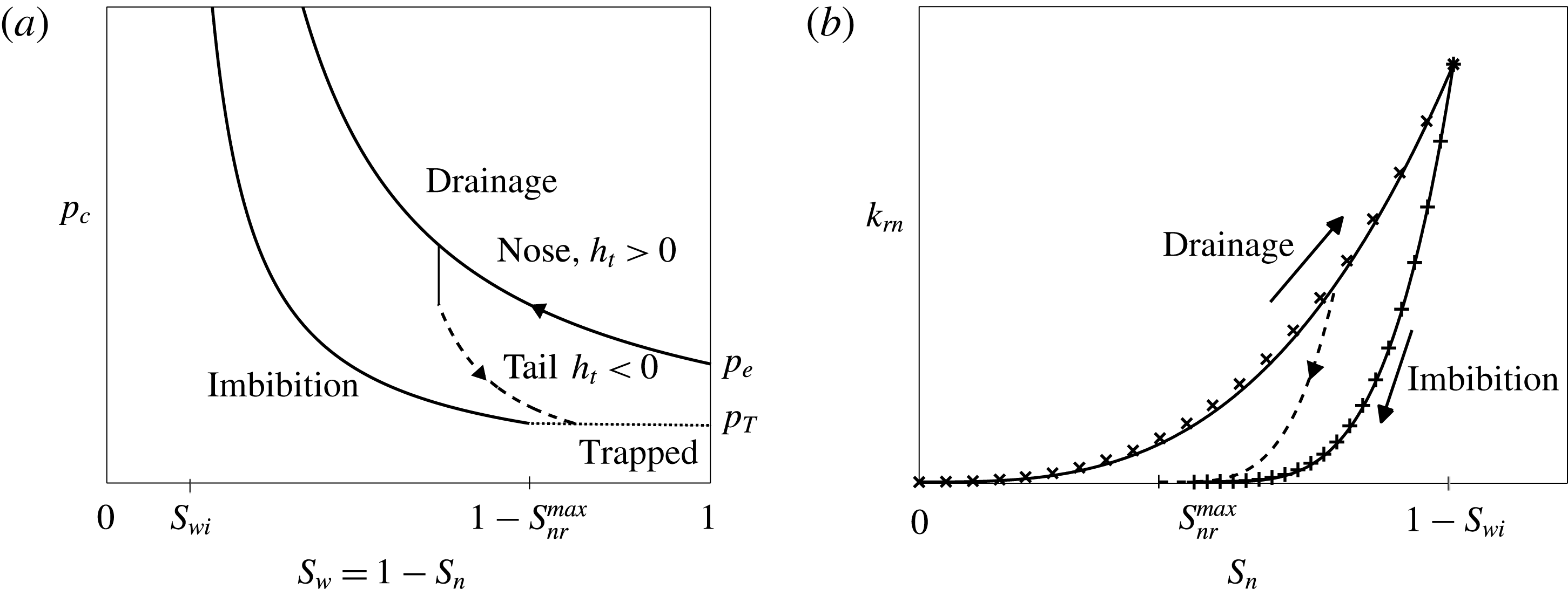
as the current evolves. Example curves for (2.1), (2.3) and (2.4) are sketched in figure 2(a) for the case
 $\unicode[STIX]{x1D6EC}_{I}=\unicode[STIX]{x1D6EC}_{D}=1$
and with numerical values given in the caption.
Primary drainage and imbibition bounding curves (solid), with an example scanning curve (dashed) for (a) capillary pressure and (b) relative permeability. (a) The capillary pressure parameters for this particular presentation are
 $\unicode[STIX]{x1D6EC}_{I}=\unicode[STIX]{x1D6EC}_{D}=1$
, with
 $p_{e}/p_{T}=2$
,
 $S_{wi}=0.1$
and
 $S_{nr}^{max}=0.3$
. The discontinuous drop in capillary pressure
 $\unicode[STIX]{x0394}p=p_{e}-p_{T}$
is seen at the transition from primary drainage to secondary imbibition. (b) The relative permeability parameters are
 $\unicode[STIX]{x1D6FC}_{D}=3$
,
 $\unicode[STIX]{x1D6FC}_{I}=4$
and
 $k_{rn0}=0.26$
, with
 $S_{wi}=0.42$
and
 $S_{nr}^{max}=0.3$
to fit empirical data from a sandstone core sample from Alberta, Canada, plotted for primary drainage (
 $\times$
) and primary imbibition (
 $+$
) (Bennion & Bachu Reference Bennion and Bachu2006).
Since pressures are nearly hydrostatic within the current, the vertical gradient of capillary pressure is linear and proportional to the density difference between the two fluids,
 $\unicode[STIX]{x0394}\unicode[STIX]{x1D70C}$
and the gravitational acceleration,
 $g$
. The capillary pressure is therefore given by
 $$\begin{eqnarray}\displaystyle p_{c}(h,z) & = & \displaystyle p_{e}+(h-z)\unicode[STIX]{x0394}\unicode[STIX]{x1D70C}g\quad (r>r_{b})\end{eqnarray}$$
 $$\begin{eqnarray}\displaystyle p_{c}(h,z) & = & \displaystyle p_{T}+(h-z)\unicode[STIX]{x0394}\unicode[STIX]{x1D70C}g\quad (r<r_{b}),\end{eqnarray}$$
 $z=h$
) the capillary pressure is equal to the entry pressure,
 $p_{e}$
and at the boundary in the receding region, where fluid is at residual saturation, the capillary pressure is equal to the terminal pressure,
 $p_{T}$
.
By combining the assumption of hydrostatic pressure in each phase with the definition of the capillary pressure we can define effective saturations for drainage and imbibition respectively, written as
 $$\begin{eqnarray}s_{\mathit{eff}}^{j}(h,z)=1-(p_{c}/p_{j})^{-\unicode[STIX]{x1D6EC}_{j}}=1-\left(1+\frac{h-z}{h_{j}}\right)^{-\unicode[STIX]{x1D6EC}_{j}}\quad (j=D,I)\end{eqnarray}$$
for notational convenience, where
 $p_{D}\equiv p_{e}$
,
 $p_{I}\equiv p_{T}$
, the height scale
 $h_{D}\equiv h_{e}=p_{e}/\unicode[STIX]{x0394}\unicode[STIX]{x1D70C}g$
is the characteristic capillary entry height and
 $h_{I}\equiv h_{T}=p_{T}/\unicode[STIX]{x0394}\unicode[STIX]{x1D70C}g$
is the equivalent characteristic terminal height during imbibition. The height scales
 $h_{e}$
and
 $h_{T}$
indicate the relative strength of capillary forces to gravity during drainage and imbibition.
Thus, we find the drainage saturation distribution by rearranging (2.1) and substituting (2.6a ) to obtain
 $$\begin{eqnarray}s^{D}=s_{\mathit{eff}}^{D}[h(r,t),z].\end{eqnarray}$$
Hence the historical maximum saturation distribution everywhere is known to be
 $$\begin{eqnarray}s^{\prime }=s_{\mathit{eff}}^{D}[h_{\mathit{max}}(r),z].\end{eqnarray}$$
Similarly, we find the imbibition saturation distribution by rearranging (2.4) and substituting (2.6b
). By setting the resultant expression equal to (2.8) when
 $h=h_{\mathit{max}}$
, we find that the asymptote
 $s_{a}=s_{r}+(s^{\prime }-s_{r})/s_{\mathit{eff}}^{I}$
and hence the imbibition saturation distribution is given by
 $$\begin{eqnarray}s^{I}=(1-\unicode[STIX]{x1D70F})\frac{s_{\mathit{eff}}^{D}(h_{max},z)}{s_{\mathit{eff}}^{I}(h_{max},z)}s_{\mathit{eff}}^{I}(h,z)+s_{r},\end{eqnarray}$$
where the trapping fraction
 $\unicode[STIX]{x1D70F}$
is defined by
 $$\begin{eqnarray}\unicode[STIX]{x1D70F}=s_{r}(s^{\prime })/s^{\prime }\end{eqnarray}$$
and describes the fraction of the fluid initially in a pore at the point of flow reversal that is ultimately residually trapped.
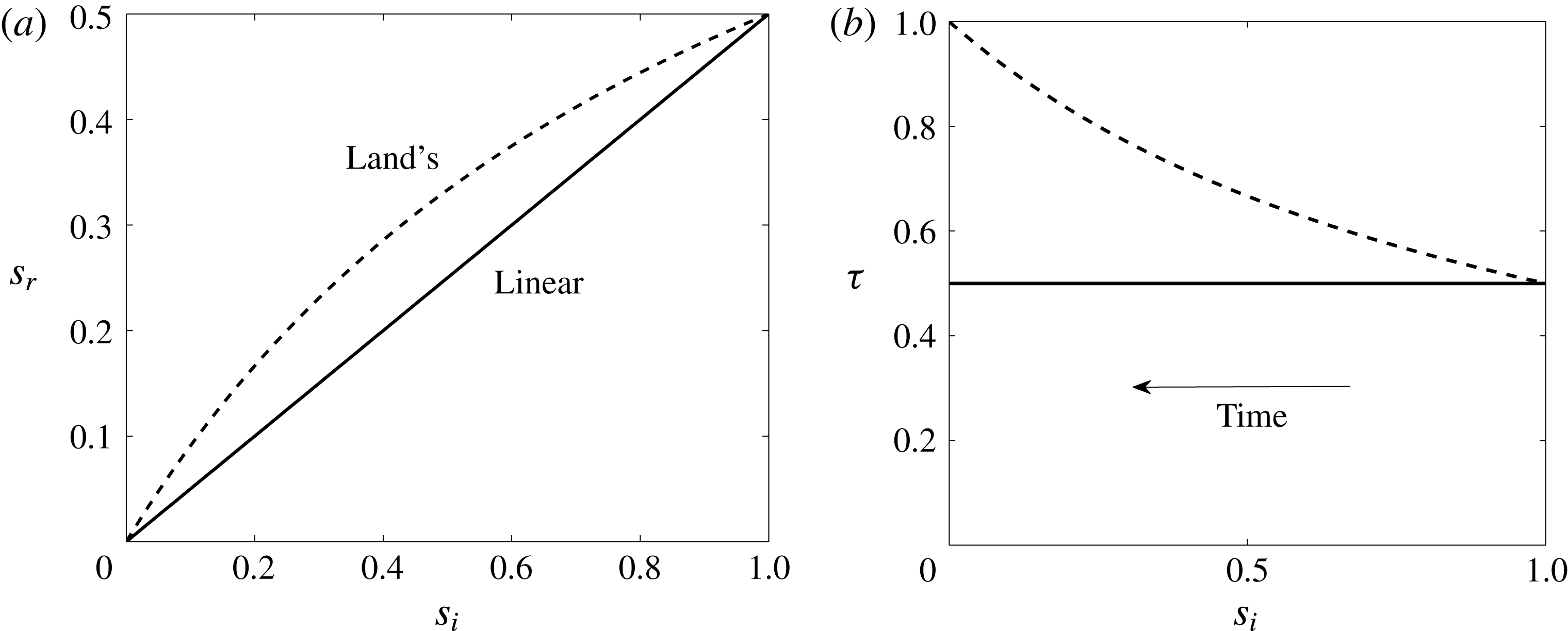
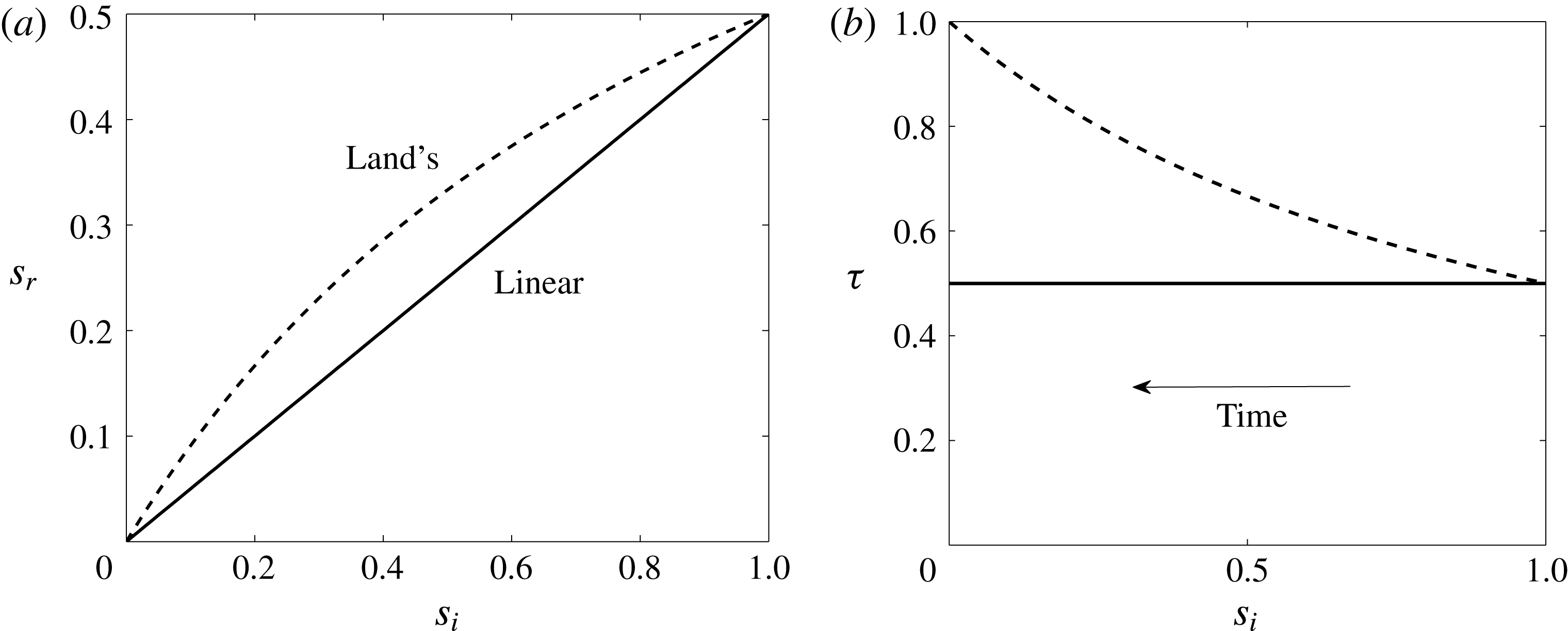
(a) The residual saturation and (b) the corresponding trapping fraction plotted against initial saturation for two examples of simple trapping models when
 $s_{r}^{\mathit{max}}=0.5$
. In both graphs, the linear trapping model, defined by (2.11), is indicated by the solid line, and Land’s model, defined by (2.12) and (2.13), with
 ${\hat{C}}=1$
, by the dashed curve.
2.3 Trapping models
Here we give a brief introduction to trapping models and define the two specific models we use to illustrate our results in this paper.
The trapping model used to capture the empirical relationship between initial and residual saturation can fundamentally change predictions for the long-term behaviour of two-phase gravity currents due to its influence on the saturation profile in the receding region (2.9). Empirical evidence suggests that the residual saturation
 $s_{r}$
, and therefore the trapping fraction
 $\unicode[STIX]{x1D70F}$
, depends on the historical maximum saturation up to the time of flow reversal,
 $s^{\prime }$
. Pentland et al. (Reference Pentland, Al-Mansoori, Iglauer, Bijeljic and Blunt2008) provide a broad overview of trapping models.
The simplest trapping models are characterised by the irreducible wetting phase saturation
 $S_{wi}$
and the maximum residual non-wetting phase saturation
 $S_{nr}^{max}$
, each determined from primary drainage and imbibition processes respectively. Examples are indicated on the horizontal saturation axis in figure 2. In this study we use two models to illustrate the significant effect that the trapping relation has on the long-term behaviour of the gravity current resulting from a finite release of fluid, although alternative trapping models for specific fluid–rock systems can be readily used.
The linear trapping model is defined by
 $$\begin{eqnarray}s_{r}=s_{r}^{\mathit{max}}s_{i},\end{eqnarray}$$
which also depends on the irreducible wetting phase saturation via (2.2), and describes a relation where the trapping fraction
 $\unicode[STIX]{x1D70F}$
remains constant regardless of the initial saturation. The linear trapping relation and fraction are plotted using a solid line in figures 3(a) and 3(b) respectively, where
 $s_{r}^{\mathit{max}}=0.5$
. Uniform saturation models, which incorporate fluid being trapped at a uniform residual saturation, also exhibit a constant trapping fraction (for example Kochina et al.
Reference Kochina, Mikhailov and Filinov1983) and this analogy becomes important later in this paper.
We also consider the commonly used nonlinear model, introduced by Land (Reference Land1968). Land’s model relates the initial saturation to the residual saturation by
 $$\begin{eqnarray}s_{r}=s_{i}/(1+{\hat{C}}s_{i}),\end{eqnarray}$$
where the constant
 $$\begin{eqnarray}{\hat{C}}=(1-s_{r}^{max})/s_{r}^{max},\end{eqnarray}$$
also depends on the irreducible wetting phase saturation via (2.2). Land’s model captures the common characteristics that the residual saturation decreases and notably the trapping fraction increases with decreasing initial saturation. This is visualised by the dashed curve plotted in figures 3(a) and 3(b), where
 $s_{r}^{\mathit{max}}=0.5$
, or
 ${\hat{C}}=1$
. We shall see below that this enhanced trapping efficiency at lower maximum saturations leads to significantly different long-time behaviour of the gravity current.
2.4 Evolution of the height of the current
In this subsection we derive the key components of the governing equation for a two-phase gravity current resulting from an instantaneous release of fluid, the so-called saturation and flux functions, which incorporate the pore-scale physics within the drainage and imbibition regions.
The rate of change of the height of the current,
 $h$
, at a given radial position is related to the divergence of the depth-integrated flux. The depth-integrated, two-phase gravity current model for radial spreading was derived by Golding et al. (Reference Golding, Huppert and Neufeld2013) and is given by
 $$\begin{eqnarray}\unicode[STIX]{x1D711}{\mathcal{R}}\frac{\unicode[STIX]{x2202}h}{\unicode[STIX]{x2202}t}-\frac{u_{b}}{r}\frac{\unicode[STIX]{x2202}}{\unicode[STIX]{x2202}r}\left(r{\mathcal{F}}h\frac{\unicode[STIX]{x2202}h}{\unicode[STIX]{x2202}r}\right)=0,\end{eqnarray}$$
where
 $u_{b}=kk_{rn0}\unicode[STIX]{x0394}\unicode[STIX]{x1D70C}g/\unicode[STIX]{x1D707}_{n}$
is the buoyancy velocity,
 $\unicode[STIX]{x1D711}=\unicode[STIX]{x1D719}(1-S_{wi})$
is the saturation adjusted porosity of the porous medium and
 ${\mathcal{R}}$
and
 ${\mathcal{F}}$
are dimensionless functions of
 $h$
defined by
 $$\begin{eqnarray}{\mathcal{R}}=\int _{0}^{h}\frac{\unicode[STIX]{x2202}s}{\unicode[STIX]{x2202}h}\,\text{d}z,\quad {\mathcal{F}}=\frac{1}{k_{rn0}h}\int _{0}^{h}k_{rn}(s)\,\text{d}z.\end{eqnarray}$$
The saturation function
 ${\mathcal{R}}$
captures how the volume of fluid changes in the current per unit area as the height changes and the flux function
 ${\mathcal{F}}$
adjusts the flux term to account for the reduced permeability of fluid in a two-phase gravity current by integrating the non-wetting phase relative permeability
 $k_{rn}$
. In contrast to the constant-flux case studied previously, where there is only an advancing drainage front, the finite-volume current considered here has two sets of saturation and flux functions due to the hysteresis between drainage and secondary imbibition in the advancing and receding regions.
The drainage saturation function in the advancing region of the current is given by
 $$\begin{eqnarray}{\mathcal{R}}^{D}(h/h_{e})=[1-(1+h/h_{e})^{-\unicode[STIX]{x1D6EC}_{D}}]=s_{\mathit{eff}}^{D}(h,0),\end{eqnarray}$$
which is the non-wetting phase saturation at
 $z=0$
used in Golding et al. (Reference Golding, Neufeld, Hesse and Huppert2011, Reference Golding, Huppert and Neufeld2013) and found by substituting (2.7) into (2.15a
). In the receding region for secondary imbibition we find, by substituting (2.9) into (2.15a
), that the saturation function is given by
 $$\begin{eqnarray}{\mathcal{R}}^{I}(h/h_{T},h_{max}/h_{e})=\int _{0}^{h}\frac{\unicode[STIX]{x1D6EC}_{I}}{h_{T}}(1-\unicode[STIX]{x1D70F})\frac{s_{\mathit{eff}}^{D}(h_{\mathit{max}},z)}{s_{\mathit{eff}}^{I}(h_{\mathit{max}},z)}[1-s_{\mathit{eff}}^{I}(h,z)]^{-\frac{(\unicode[STIX]{x1D6EC}_{I+1})}{\unicode[STIX]{x1D6EC}_{I}}}\,\text{d}z.\end{eqnarray}$$
The relative permeability in each region determines the flux function and, as in previous studies, we employ a commonly used power-law relation of saturation for primary drainage, defined by
 $$\begin{eqnarray}k_{rn}^{D}(s)=k_{rn0}s^{\unicode[STIX]{x1D6FC}_{D}},\end{eqnarray}$$
where
 $k_{rn0}$
is the endpoint relative permeability which occurs at the maximum non-wetting phase saturation,
 $1-S_{wi}$
, and
 $\unicode[STIX]{x1D6FC}_{D}$
is an empirically determined constant. During secondary imbibition, as saturation decreases, the path of descent of relative permeability depends on the maximum saturation at the point of flow reversal,
 $s^{\prime }$
, and similarly to capillary pressure this is represented by scanning curves. It is important to note that at the end of this process, the relative permeability of the non-wetting phase is zero at the residual saturation
 $s_{r}(s^{\prime })$
, which can range between
 $0$
and
 $s_{r}^{max}$
depending on
 $s^{\prime }$
. In this study, we use the history-dependent model for relative permeability proposed by Killough (Reference Killough1976) for use in petroleum reservoir simulations because it provides a mathematically simple expression for linking relative permeability as drainage transitions into imbibition. It was also employed by Juanes et al. (Reference Juanes, Spiteri, Orr and Blunt2006) in their study of relative permeability hysteresis in models for the geological storage of
 $\text{CO}_{2}$
. However, we note that our framework is not limited to this particular model. The secondary imbibition relative permeability is defined by
 $$\begin{eqnarray}k_{rn}^{I}(s)=k_{rn}^{D}(s^{\prime })\left(\frac{s-s_{r}}{s^{\prime }-s_{r}}\right)^{\unicode[STIX]{x1D6FC}_{I}},\end{eqnarray}$$
where
 $\unicode[STIX]{x1D6FC}_{I}$
is the constant in the primary imbibition relative permeability curve when
 $s_{r}=s_{r}^{\mathit{max}}$
and
 $s^{\prime }=1$
in (2.19), which is more easily determined experimentally. Example relative permeability curves for primary drainage and imbibition, measured from a core sample of sandstone from Alberta, Canada are plotted in figure 2(b). Solid curves show the model bounding curves using (2.18) and (2.19), where
 $\unicode[STIX]{x1D6FC}_{D}=3$
and
 $\unicode[STIX]{x1D6FC}_{I}=4$
have been chosen to fit the experimental data. An example secondary imbibition scanning curve using (2.19) is plotted by the dashed curve for flow reversal at
 $s^{\prime }=0.5$
.
Thus returning to the flux function, we now substitute (2.7), (2.9), (2.18) and (2.19) into (2.15b ) to find that
 $$\begin{eqnarray}{\mathcal{F}}^{D}(h/h_{e})=\frac{1}{h}\int _{0}^{h}[s_{\mathit{eff}}^{D}(h,z)]^{\unicode[STIX]{x1D6FC}_{D}}\,\text{d}z,\end{eqnarray}$$
and
 $$\begin{eqnarray}{\mathcal{F}}^{I}(h/h_{T},h_{max}/h_{e},h_{max}/h_{T})=\frac{1}{h}\int _{0}^{h}\frac{[s_{\mathit{eff}}^{D}(h_{\mathit{max}},z)]^{\unicode[STIX]{x1D6FC}_{D}}}{[s_{\mathit{eff}}^{I}(h_{\mathit{max}},z)]^{\unicode[STIX]{x1D6FC}_{I}}}[s_{\mathit{eff}}^{I}(h,z)]^{\unicode[STIX]{x1D6FC}_{I}}\,\text{d}z,\end{eqnarray}$$
in the advancing and retreating regions respectively.
2.5 Boundary and initial conditions
Here we complete the model definition by specifying boundary conditions.
There are five spatial boundary conditions for a gravity current resulting from the release of a finite volume of fluid. There is a condition of no flux through the nose of the current, where the height is zero, and no flux input at the origin,
 $$\begin{eqnarray}h{\mathcal{F}}^{D}\frac{\unicode[STIX]{x2202}h}{\unicode[STIX]{x2202}r}=0,\quad h=0\quad (r=r_{N}),\quad h{\mathcal{F}}^{I}\frac{\unicode[STIX]{x2202}h}{\unicode[STIX]{x2202}r}=0\quad (r=0).\end{eqnarray}$$
Continuity of height and flux are also explicitly enforced at the boundary dividing regions of drainage and imbibition,
 $r=r_{b}$
, by
 $$\begin{eqnarray}h|_{r_{b}^{-}}=h|_{r_{b}^{+}},\quad \left.h{\mathcal{F}}^{I}\frac{\unicode[STIX]{x2202}h}{\unicode[STIX]{x2202}r}\right|_{r_{b}^{-}}=\left.h{\mathcal{F}}^{D}\frac{\unicode[STIX]{x2202}h}{\unicode[STIX]{x2202}r}\right|_{r_{b}^{+}},\end{eqnarray}$$
respectively. Saturation profiles are defined to be equal when
 $h=h_{max}$
, i.e. at
 $r=r_{b}$
, and therefore the flux functions are continuous here. Thus we deduce from (2.23a,b
) that the gradient of the current height,
 $\unicode[STIX]{x2202}h/\unicode[STIX]{x2202}r$
, is continuous at
 $r=r_{b}$
.
The initial shape of the gravity current must also be supplied to fully define the problem. If we suppose that the initial volume of fluid,
 $V$
, is held in an axisymmetric shape with height profile
 $h_{0}(r)$
, extending between
 $r=0$
and
 $r=r_{0}$
, then the initial mass (or volume) may be expressed as
 $$\begin{eqnarray}2\unicode[STIX]{x03C0}\unicode[STIX]{x1D711}\int _{0}^{r_{0}}\int _{0}^{h_{0}}s_{0}[h_{0}(r),z]\,\text{d}zr\,\text{d}r=V,\end{eqnarray}$$
where
 $s_{0}[h_{0}(r),z]$
is the initial saturation distribution. In practice, the initial shape might be that of the slumping groundwater mound, or the shape of the
 $\text{CO}_{2}$
plume at the end of injection, for example, in which case
 $s_{0}=s^{D}(h_{0},z)$
defined by (2.7).
2.6 Scaling and non-dimensionalisation
We are able to simplify the model in this subsection by applying scaling analysis.
The solution for the height profile of the two-phase gravity current depends on the characteristic variables
 $r$
and
 $t$
, the buoyancy velocity,
 $u_{b}$
, the initial volume of fluid released,
 $V$
, the initial radius of the volume,
 $r_{0}$
, the capillary pressure curve parameters
 $h_{e}$
,
 $h_{T}$
,
 $\unicode[STIX]{x1D6EC}_{D}$
and
 $\unicode[STIX]{x1D6EC}_{I}$
, relative permeability curve parameters
 $\unicode[STIX]{x1D6FC}_{D}$
and
 $\unicode[STIX]{x1D6FC}_{I}$
and the normalised maximum residual saturation,
 $s_{r}^{\mathit{max}}$
. All saturations have been already scaled using the irreducible wetting phase saturation,
 $S_{wi}$
. The height of the initial volume of fluid is determined given the initial radius, volume and equilibrium saturation distribution. Although the number of parameters is large, the complexity of the problem can be reduced by some sensible scaling.
By applying scaling analysis to (2.14) and (2.24) and rearranging, we find the following relations between the dimensions of radius, height, time, permeability, porosity and the constant characteristic parameters
 $$\begin{eqnarray}\langle r\rangle ^{4}\sim \frac{V\unicode[STIX]{x0394}\unicode[STIX]{x1D70C}g}{\unicode[STIX]{x1D707}_{n}}\langle t\rangle \frac{\langle \text{perm}\rangle }{\langle \text{poros}\rangle ^{2}}\quad \text{and}\quad \langle h\rangle \sim V\langle \text{poros}\rangle ^{-1}\langle r\rangle ^{-2},\end{eqnarray}$$
where
 $\langle .\rangle$
denotes ‘scales as’, the permeability
 $\langle \text{perm}\rangle \sim kk_{rn0}\langle {\mathcal{F}}\rangle$
and porosity
 $\langle \text{poros}\rangle \sim \unicode[STIX]{x1D711}\langle {\mathcal{R}}\rangle \sim \unicode[STIX]{x1D711}\langle s\rangle$
. For comparison, we note that for single-phase gravity currents
 $\langle \text{perm}\rangle \equiv k$
and
 $\langle \text{poros}\rangle \equiv \unicode[STIX]{x1D719}$
. In contrast for two-phase gravity currents,
 $\langle \text{perm}\rangle$
and
 $\langle \text{poros}\rangle$
are complex, nonlinear functions of
 $h$
in general. In certain circumstances in the long-time limit, these functions can be simplified, which leads to self-similar behaviour of the current, as discussed in § 3.1.
We denote horizontal and vertical length scales by
 $R$
and
 $H$
respectively and the time scale by
 $T$
, and by ignoring the functional components of (2.25a,b
), define dimensionless variables
 $$\begin{eqnarray}\hat{r}=r/R,\quad \hat{z}=z/H,\quad {\hat{h}}=h/H,\quad \hat{t}=t/T,\end{eqnarray}$$
where
 $$\begin{eqnarray}R=r_{0},\quad H=\frac{V}{\unicode[STIX]{x1D711}r_{0}^{2}},\quad T=\frac{r_{0}^{4}\unicode[STIX]{x1D711}^{2}}{Vu_{b}}.\end{eqnarray}$$
Thus the radial extent of all currents and the height of the current are scaled by the initial radius, the fluid volume and the effective porosity, while the time scale is found in terms of the buoyancy velocity from (2.14).
The system is now characterised by two key dimensionless parameters. First, the Bond number
 $$\begin{eqnarray}B\equiv \frac{\unicode[STIX]{x0394}\unicode[STIX]{x1D70C}gH}{p_{e}}=\frac{H}{h_{e}}=\frac{V}{\unicode[STIX]{x1D711}r_{0}^{2}h_{e}},\end{eqnarray}$$
indicates the relative strength of gravity to capillary forces at
 $t=0$
. We note that as the fluid spreads and the height of the current decreases with time, the relative strength of capillary forces increases and therefore a time-dependent Bond number would decrease with time. Second, capillary hysteresis is characterised by
 $$\begin{eqnarray}\unicode[STIX]{x1D6FF}=h_{e}/h_{T},\end{eqnarray}$$
which is the ratio of the entry to terminal capillary pressure. These two pressures are generally related and Gerhard & Kueper (Reference Gerhard and Kueper2003) determined experimentally that
 $\unicode[STIX]{x1D6FF}\approx 5/3$
, and for most realistic situations
 $\unicode[STIX]{x1D6FF}\geqslant 1$
.
We now use the dimensionless and normalised quantities (2.27)–(2.29) to obtain a set of equations to solve for
 ${\hat{h}}$
, formulated in terms of variables
 $\hat{r}$
,
 $\hat{t}$
,
 $\hat{z}$
and the non-wetting saturation
 $s$
. The dimensionless parameters are
 $B$
and
 $\unicode[STIX]{x1D6FF}$
, which characterise the physical balance between capillary forces and gravity, along with
 $\unicode[STIX]{x1D6EC}_{D}$
,
 $\unicode[STIX]{x1D6EC}_{I}$
,
 $\unicode[STIX]{x1D6FC}_{D}$
,
 $\unicode[STIX]{x1D6FC}_{I}$
and
 $s_{r}^{max}$
, which characterise the functional form of the constitutive relations for capillary pressure, relative permeability and residual trapping. Hereafter we drop the hats on dimensionless variables for ease of notation.
The dimensionless model of the spreading and trapping of a two-phase current can therefore be written by substituting (2.26)–(2.29) into (2.14) to find
 $$\begin{eqnarray}{\mathcal{R}}\frac{\unicode[STIX]{x2202}h}{\unicode[STIX]{x2202}t}-\frac{1}{r}\frac{\unicode[STIX]{x2202}}{\unicode[STIX]{x2202}r}\left[rh\frac{\unicode[STIX]{x2202}h}{\unicode[STIX]{x2202}r}{\mathcal{F}}\right]=0.\end{eqnarray}$$
Here (2.16) and (2.17) are rewritten as
 $$\begin{eqnarray}\displaystyle {\mathcal{R}}=\left\{\begin{array}{@{}ll@{}}{\mathcal{R}}^{D}(Bh,\unicode[STIX]{x1D6EC}_{D})\quad & (r>r_{b})\\ {\mathcal{R}}^{I}(\unicode[STIX]{x1D6FF}Bh,Bh_{max},\unicode[STIX]{x1D6FF}Bh_{max},\unicode[STIX]{x1D6FF},\unicode[STIX]{x1D6EC}_{D},\unicode[STIX]{x1D6EC}_{I},s_{r}^{max})\quad & (r<r_{b})\end{array}\right. & & \displaystyle\end{eqnarray}$$
and (2.20) and (2.21) are rewritten as
 $$\begin{eqnarray}\displaystyle {\mathcal{F}}=\left\{\begin{array}{@{}ll@{}}{\mathcal{F}}^{D}(Bh,\unicode[STIX]{x1D6EC}_{D},\unicode[STIX]{x1D6FC}_{D})\quad & (r>r_{b})\\ {\mathcal{F}}^{I}(\unicode[STIX]{x1D6FF}Bh,Bh_{max},\unicode[STIX]{x1D6FF}Bh_{max},\unicode[STIX]{x1D6FF},\unicode[STIX]{x1D6EC}_{D},\unicode[STIX]{x1D6EC}_{I},\unicode[STIX]{x1D6FC}_{D},\unicode[STIX]{x1D6FC}_{I})\quad & (r<r_{b}).\end{array}\right. & & \displaystyle\end{eqnarray}$$
The boundary conditions (2.22) and (2.23) are rewritten here in dimensionless variables for completeness,
 $$\begin{eqnarray}h\frac{\unicode[STIX]{x2202}h}{\unicode[STIX]{x2202}r}=0,\quad h=0\quad (r=r_{N}),\quad \frac{\unicode[STIX]{x2202}h}{\unicode[STIX]{x2202}r}=0\quad (r=0),\end{eqnarray}$$
and
 $$\begin{eqnarray}h|_{r_{b}^{-}}=h|_{r_{b}^{+}},\quad \left.h{\mathcal{F}}^{I}\frac{\unicode[STIX]{x2202}h}{\unicode[STIX]{x2202}r}\right|_{r_{b}^{-}}=\left.h{\mathcal{F}}^{D}\frac{\unicode[STIX]{x2202}h}{\unicode[STIX]{x2202}r}\right|_{r_{b}^{+}}.\end{eqnarray}$$
Finally, the dimensionless initial mass (or volume) is
 $$\begin{eqnarray}2\unicode[STIX]{x03C0}\int _{0}^{1}\int _{0}^{h_{0}}s^{D}[h_{0}(r),z]\,\text{d}zr\,\text{d}r=1.\end{eqnarray}$$
We have thus derived the set of equations (2.30)–(2.32) and boundary conditions (2.33)–(2.35) which govern the spreading of a two-phase gravity current resulting from an instantaneous release of fluid. We explore solutions for various scenarios throughout the following section, paying particular attention to the choice of trapping model.
3 Spreading of a two-phase finite-release gravity current
We developed in § 2 a very general framework which permits the use of any empirical constitutive relations for capillary pressure, relative permeability and residual trapping. In general, the model must be solved numerically due to the nonlinear nature of the equations and the dependence on historical information through the saturation distribution. However, in the long-time limit when there is no hysteresis and the trapping relation is linear, the problem reduces in complexity. The model admits a similarity solution of the second kind, similar to those derived by Van Dijke & Van der Zee (Reference Van Dijke and Van der Zee1997) and Bear & Ryzhik (Reference Bear and Ryzhik1998), and the two-phase analogue of the groundwater mound model presented by Kochina et al. (Reference Kochina, Mikhailov and Filinov1983), which we summarise in § 3.1. We validate this long-time similarity solution by solving the full two-phase model numerically with a linear trapping model in § 3.2. Next, we demonstrate the vital importance of the choice of trapping model in § 3.3 by using numerical computations with Land’s trapping relation to show how the current slows down in the long-time limit, in stark contrast to the self-similar spreading with the linear trapping model. The results of § 3.1 argue that when Land’s trapping model is used, the model predicts that the two-phase gravity current will eventually stop. The approach to the steady state is indeed suggested by our long-time numerical results.
3.1 Linear trapping: self-similar spreading in the long-time limit
In this subsection, we investigate the effect of using a linear trapping model, defined by (2.11), on the spreading of a multiphase gravity current in the long-time limit, which we find to be self-similar.
Here we consider a scenario where hysteresis in capillary pressure curves is caused only by the existence of residual trapping, i.e.
 $\unicode[STIX]{x1D6EC}_{D}=\unicode[STIX]{x1D6EC}_{I}=\unicode[STIX]{x1D6EC}$
and
 $\unicode[STIX]{x1D6FF}=1$
. In this case, the rate of change of imbibition saturation with height (the integrand of the saturation function (2.15a
)) simplifies to
 $\unicode[STIX]{x2202}s^{I}(h,z)/\unicode[STIX]{x2202}h=(1-\unicode[STIX]{x1D70F})\unicode[STIX]{x2202}s_{\mathit{eff}}^{I}(h,z)/\unicode[STIX]{x2202}h$
, yet in general retains its dependence on historical saturation and therefore height information through
 $\unicode[STIX]{x1D70F}$
. However, when the trapping fraction is constant, there is no dependence on historical saturation and the saturation function is history independent. Similarly, if relative permeability curves are parameterised by
 $\unicode[STIX]{x1D6FC}_{D}=\unicode[STIX]{x1D6FC}_{I}=\unicode[STIX]{x1D6FC}$
in both regions and the trapping fraction is constant, the flux function too does not depend on history. Thus, the extra length scale
 $h_{\mathit{max}}$
is removed from the problem. Furthermore, as the current spreads and its height decreases monotonically,
 $\unicode[STIX]{x1D6EC}Bh\ll 1$
in the long-time limit and the saturation distribution in each region is approximately linear with distance from the current boundary,
 $s^{D}\approx \unicode[STIX]{x1D6EC}B(h-z)$
and
 $s^{I}\approx (1-\unicode[STIX]{x1D70F})\unicode[STIX]{x1D6EC}B(h-z)+\unicode[STIX]{x1D70F}\unicode[STIX]{x1D6EC}B(h_{\mathit{max}}-z)$
in the drainage and imbibition regions respectively. Consequently the saturation and flux functions are approximated by power laws, given by
 $$\begin{eqnarray}{\mathcal{R}}^{D}\approx \unicode[STIX]{x1D6EC}Bh,\quad {\mathcal{F}}^{D}\approx \frac{1}{1+\unicode[STIX]{x1D6FC}}(\unicode[STIX]{x1D6EC}Bh)^{\unicode[STIX]{x1D6FC}},\end{eqnarray}$$
and
 $$\begin{eqnarray}{\mathcal{R}}^{I}\approx (1-\unicode[STIX]{x1D70F}){\mathcal{R}}^{D},\quad F^{I}\approx F^{D}.\end{eqnarray}$$
Thus in the long-time limit when there is no hysteresis the current spreads in a self-similar fashion. History dependence in the imbibition region can also disappear when there is hysteresis but an even longer-time limit must be considered where the height in the drainage region has also decreased such that
 $\unicode[STIX]{x1D6EC}_{D}Bh_{\mathit{max}}\ll 1$
.
In order to perform dimensional analysis in the long-time limit, we substitute (3.1a,b ) and (3.2a,b ) into the dimensional governing equation (2.14) to obtain
 $$\begin{eqnarray}h\frac{\unicode[STIX]{x2202}h}{\unicode[STIX]{x2202}t}=c\frac{u_{b}}{\unicode[STIX]{x1D711}(1+\unicode[STIX]{x1D6FC})}\left(\frac{\unicode[STIX]{x1D6EC}B}{H}\right)^{\unicode[STIX]{x1D6FC}-1}\frac{1}{r}\frac{\unicode[STIX]{x2202}}{\unicode[STIX]{x2202}r}\left[rh^{\unicode[STIX]{x1D6FC}+1}\frac{\unicode[STIX]{x2202}h}{\unicode[STIX]{x2202}r}\right],\end{eqnarray}$$
where
 $H$
and
 $B$
are defined by (2.27b
) and (2.28) respectively, and
 $$\begin{eqnarray}c=\left\{\begin{array}{@{}ll@{}}c_{I}=1/(1-s_{r}^{\mathit{max}})\quad & (\unicode[STIX]{x2202}h/\unicode[STIX]{x2202}t<0)\\ c_{D}=1\quad & (\unicode[STIX]{x2202}h/\unicode[STIX]{x2202}t>0).\end{array}\right.\end{eqnarray}$$
When there is no trapping,
 $s_{r}^{\mathit{max}}=0$
, which means that
 $c_{I}=c_{D}$
and so there is only one equation governing the evolution of the spreading current.
In the manner of Kochina et al. (Reference Kochina, Mikhailov and Filinov1983) and Barenblatt (Reference Barenblatt1996), scaling analysis is used to find three dimensionless combinations of the characteristic parameters,
 $$\begin{eqnarray}\unicode[STIX]{x1D709}=rL^{-1},\quad \unicode[STIX]{x1D709}_{0}=r_{0}L^{-1}\quad \text{and}\quad c_{D}/c_{I}=1-s_{r}^{\mathit{max}}.\end{eqnarray}$$
In this long-time limit,
 $\langle \text{perm}\rangle =kk_{rn0}(\unicode[STIX]{x1D6EC}B\langle h\rangle /H)^{\unicode[STIX]{x1D6FC}}$
and
 $\langle \text{poros}\rangle =\unicode[STIX]{x1D711}\unicode[STIX]{x1D6EC}B\langle h\rangle /H$
and hence the scaling analysis in § 2.6 shows that the length scale
 $L$
is given by
 $$\begin{eqnarray}L=\unicode[STIX]{x1D711}^{-1/2}\left[V_{0}^{\unicode[STIX]{x1D6FC}/2}\frac{u_{b}t}{(1-s_{r}^{\mathit{max}})}\left(\frac{\unicode[STIX]{x1D6EC}B}{H}\right)^{(\unicode[STIX]{x1D6FC}-2)/2}\right]^{1/(2+\unicode[STIX]{x1D6FC})},\end{eqnarray}$$
where the
 $1-s_{r}^{\mathit{max}}$
factor comes from the imbibition saturation function in the governing equation and the height profile has the form
 $$\begin{eqnarray}h=\left[\frac{V_{0}(1-S_{r}^{max})}{u_{b}t}\right]^{1/(2+\unicode[STIX]{x1D6FC})}\left(\frac{H}{\unicode[STIX]{x1D6EC}B}\right)^{\unicode[STIX]{x1D6FC}/(2+\unicode[STIX]{x1D6FC})}F(\unicode[STIX]{x1D709},\unicode[STIX]{x1D709}_{0},c_{D}/c_{I},\unicode[STIX]{x1D6FC}),\end{eqnarray}$$
where
 $F$
is a dimensionless height function.
When trapping occurs, the condition for global conservation of mass cannot be straightforwardly integrated to give an extra scaling condition and we must therefore seek a solution assuming incomplete self-similarity (Kochina et al.
Reference Kochina, Mikhailov and Filinov1983; Barenblatt Reference Barenblatt1996). By combining (3.5a,b
) and (3.6a,b
), and assuming that
 $F$
has the form
 $F(\unicode[STIX]{x1D709},\unicode[STIX]{x1D709}_{0},c_{D}/c_{I},\unicode[STIX]{x1D6FC})=\unicode[STIX]{x1D709}_{0}^{\unicode[STIX]{x1D6FE}}f(\unicode[STIX]{x1D709}\unicode[STIX]{x1D709}_{0}^{-\unicode[STIX]{x1D716}},c_{D}/c_{I},\unicode[STIX]{x1D6FC})$
, we find expressions for the similarity variable, non-dimensional radius and height profiles given, after considerable algebra, by
 $$\begin{eqnarray}\unicode[STIX]{x1D701}=\hat{r}\hat{t^{\prime }}^{-\unicode[STIX]{x1D6FD}},\quad \hat{r}_{N}=\unicode[STIX]{x1D701}_{N}\hat{t^{\prime }}^{\unicode[STIX]{x1D6FD}},\quad {\hat{h}}=\unicode[STIX]{x1D701}_{N}^{2/\unicode[STIX]{x1D6FC}}(\unicode[STIX]{x1D6EC}B)^{-1/2}\hat{t^{\prime }}^{-\unicode[STIX]{x1D6E4}}f(\unicode[STIX]{x1D6F6},c_{D}/c_{I},\unicode[STIX]{x1D6FC}),\end{eqnarray}$$
where the powers of time
 $\unicode[STIX]{x1D6E4}=(\unicode[STIX]{x1D6FE}+1)/(\unicode[STIX]{x1D6FC}+2)$
and
 $\unicode[STIX]{x1D6FD}=(1-\unicode[STIX]{x1D716})/(\unicode[STIX]{x1D6FC}+2)$
,
 $\unicode[STIX]{x1D701}_{N}$
is the value of
 $\unicode[STIX]{x1D701}$
at the front of the current,
 $f$
is a dimensionless function of the normalised similarity variable
 $\unicode[STIX]{x1D6F6}=\unicode[STIX]{x1D701}/\unicode[STIX]{x1D701}_{N}$
and the factor
 $\unicode[STIX]{x1D701}_{N}^{2/\unicode[STIX]{x1D6FC}}$
in (3.7c
) is included for mathematical convenience. All the dimensionless variables are defined by (2.26), and we find a new characteristic dimensionless time
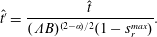 $$\begin{eqnarray}\hat{t^{\prime }}=\frac{\hat{t}}{(\unicode[STIX]{x1D6EC}B)^{(2-\unicode[STIX]{x1D6FC})/2}(1-s_{r}^{\mathit{max}})}.\end{eqnarray}$$
Hence we see that the combined effect of the Bond number and pore-size distribution,
 $B\unicode[STIX]{x1D6EC}$
, is simply to alter the time and height scales. We see from (3.7c
) that stronger capillary forces (decreasing
 $\unicode[STIX]{x1D6EC}B$
) always lead to an increased height scale. When capillary forces act to increase the height gradient through reduced saturation, but do not sufficiently reduce the relative permeability (
 $\unicode[STIX]{x1D6FC}<2$
), we see from (3.8) that the time scale decreases, whereas if relative permeability is sufficiently hindered (
 $\unicode[STIX]{x1D6FC}>2$
), the time scale of spreading increases.
Substituting (3.7a–c
) into (3.3), we obtain, after some algebra, the ordinary differential equation for the similarity profile,
 $f$
,
 $$\begin{eqnarray}\frac{\unicode[STIX]{x2202}}{\unicode[STIX]{x2202}\unicode[STIX]{x1D6F6}}\left[f^{\unicode[STIX]{x1D6FC}+1}\unicode[STIX]{x1D6F6}\frac{\unicode[STIX]{x2202}f}{\unicode[STIX]{x2202}\unicode[STIX]{x1D6F6}}\right]+{\hat{c}}(\unicode[STIX]{x1D6FC}+1)\unicode[STIX]{x1D6F6}f\left[\unicode[STIX]{x1D6E4}f+\unicode[STIX]{x1D6FD}\unicode[STIX]{x1D6F6}\frac{\unicode[STIX]{x2202}f}{\unicode[STIX]{x2202}\unicode[STIX]{x1D6F6}}\right]=0,\end{eqnarray}$$
where
 $$\begin{eqnarray}\displaystyle {\hat{c}}=\left\{\begin{array}{@{}ll@{}}1\quad & (\unicode[STIX]{x2202}h/\unicode[STIX]{x2202}t<0),\quad \text{or }(\unicode[STIX]{x1D6E4}f+\unicode[STIX]{x1D6FD}\unicode[STIX]{x1D6F6}\unicode[STIX]{x2202}f/\unicode[STIX]{x2202}\unicode[STIX]{x1D6F6}>0)\\ c_{I}/c_{D}\quad & (\unicode[STIX]{x2202}h/\unicode[STIX]{x2202}t>0),\quad \text{or }(\unicode[STIX]{x1D6E4}f+\unicode[STIX]{x1D6FD}\unicode[STIX]{x1D6F6}\unicode[STIX]{x2202}f/\unicode[STIX]{x2202}\unicode[STIX]{x1D6F6}<0)\end{array}\right. & & \displaystyle\end{eqnarray}$$
in the imbibition and drainage regions respectively. For a similarity solution to exist, the height must fall with a power of time given by
 $$\begin{eqnarray}\unicode[STIX]{x1D6E4}=(1-2\unicode[STIX]{x1D6FD})/\unicode[STIX]{x1D6FC}.\end{eqnarray}$$
Boundary conditions at the front of the current and at the origin are
 $$\begin{eqnarray}f=0\quad (\unicode[STIX]{x1D6F6}=1)\quad \text{and}\quad f^{\prime }=0\quad (\unicode[STIX]{x1D6F6}=0).\end{eqnarray}$$
To find the profile at the front of the current, we seek a solution of the drainage governing equation (3.9) of the form
 $f(\unicode[STIX]{x1D6F6})=p(1-\unicode[STIX]{x1D6F6})^{q}$
for
 $1-\unicode[STIX]{x1D6F6}\ll 1$
and obtain
 $$\begin{eqnarray}f(\unicode[STIX]{x1D6F6})=\left[\frac{c_{I}\unicode[STIX]{x1D6FC}\unicode[STIX]{x1D6FD}(1+\unicode[STIX]{x1D6FC})}{2c_{D}}\right]^{1/\unicode[STIX]{x1D6FC}}(1-\unicode[STIX]{x1D6F6})^{1/\unicode[STIX]{x1D6FC}}\quad (1-\unicode[STIX]{x1D6F6}\ll 1).\end{eqnarray}$$
We solve (3.9) numerically by shooting from
 $\unicode[STIX]{x1D6F6}=1$
using (3.12a
) and (3.13) and find the value of
 $\unicode[STIX]{x1D6FD}$
such that (3.12b
) is satisfied to a specified accuracy. In general when there is trapping,
 $s_{r}^{\mathit{max}}>0$
, the prefactor
 $\unicode[STIX]{x1D701}_{N}$
cannot be predetermined by solving (3.9), and must instead be matched with the numerical solution of the full equations.
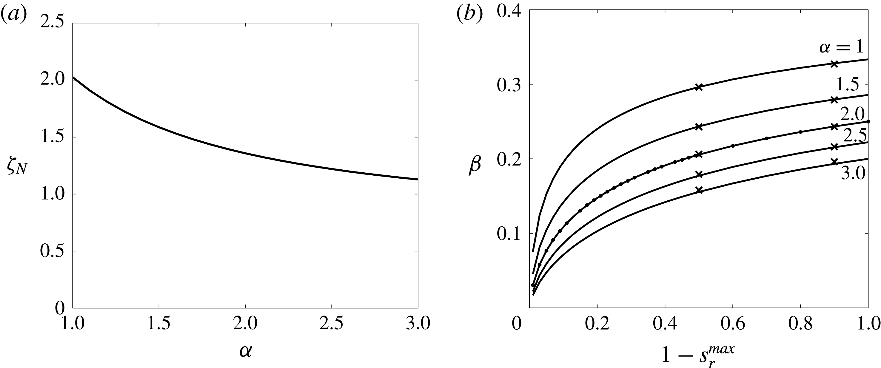
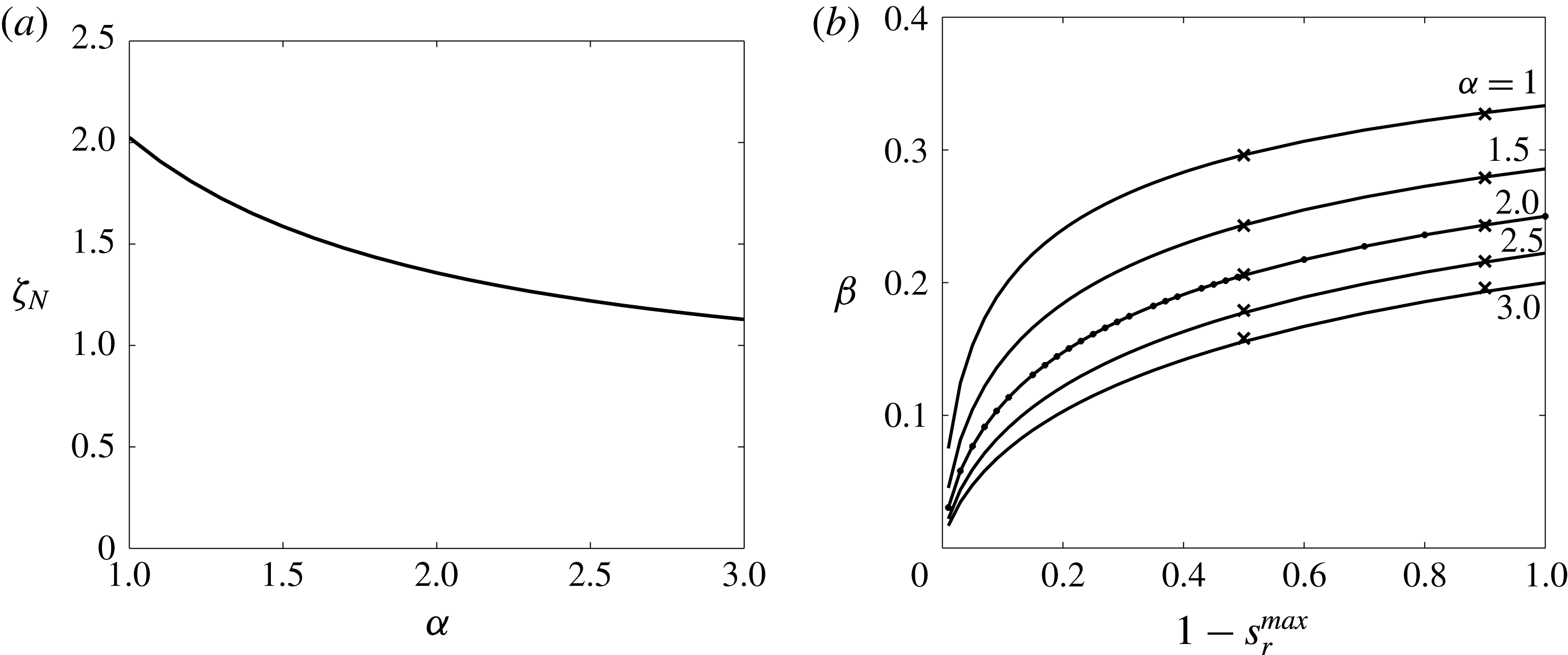
(a) Results of the similarity solution with no trapping,
 $s_{r}^{\mathit{max}}=0$
. The similarity variable at the current front,
 $\unicode[STIX]{x1D701}_{N}$
, plotted against the relative permeability power
 $\unicode[STIX]{x1D6FC}$
. The equivalent value for a single-phase current with a constant volume is
 $\unicode[STIX]{x1D701}_{N}=1.502$
(Lyle et al.
Reference Lyle, Huppert, Hallworth, Bickle and Chadwick2005). (b) With trapping,
 $s_{r}^{\mathit{max}}\geqslant 0$
. The radial rate of spreading in the solution described by
 $r\sim t^{\unicode[STIX]{x1D6FD}}$
in § 3.1 is plotted for
 $\unicode[STIX]{x1D6FC}=1,1.5,2,2.5$
and 3 as a function of
 $1-s_{r}^{\mathit{max}}$
. The equivalent values for a constant-saturation current are plotted by the black dashed curve (Kochina et al.
Reference Kochina, Mikhailov and Filinov1983). Numerical results discussed in § 3.2 are indicated by the
 $\times$
markers, for each value of
 $\unicode[STIX]{x1D6FC}$
with
 $s_{r}^{\mathit{max}}=0.1$
and 0.5.
Similar similarity solutions for the long-time limit of a three-phase, non-aqueous phase liquid lens spreading above the water table and a two-phase dense non-aqueous phase liquid lens spreading in unsaturated soil were described by Van Dijke & Van der Zee (Reference Van Dijke and Van der Zee1997) and Bear & Ryzhik (Reference Bear and Ryzhik1998). Both considered the evolution of the volume of fluid per unit lateral area, rather than the height profile described here. These studies related residual trapping to this vertically integrated volume, whereas we have used a linear initial residual saturation relation to derive the similarity solution. Bear & Ryzhik (Reference Bear and Ryzhik1998) demonstrated how the power of time in the self-similar spreading depends on the coefficient of the diffusion term (in our model
 $1-s_{r}^{\mathit{max}}$
) and is affected by a combination of the multiphase parameters from the van Genuchten capillary pressure model, along with the power of saturation in the relative permeability relation. When using the Brooks–Corey model for capillary pressure, we have found that the effect of pore-size distribution, parameterised by
 $\unicode[STIX]{x1D6EC}$
, is to alter the time scale, and is thereby removed from the similarity solution. Nevertheless, the results of Bear & Ryzhik (Reference Bear and Ryzhik1998) indicate qualitatively similar behaviour, that the power of time describing radial spreading decreases as capillary forces strengthen.
We proceed to use our solution to explore the effect of altering the relative permeability parameter
 $\unicode[STIX]{x1D6FC}$
, and the trapping fraction
 $s_{r}^{\mathit{max}}$
, on the self-similar height profile and spreading in the long-time limit. We highlight in particular the distinctive behaviour of the two-phase current depending on whether the relative permeability parameter
 $\unicode[STIX]{x1D6FC}$
is greater than, less than or equal to 2.
3.1.1 No residual trapping,
 $s_{r}^{\mathit{max}}=0$

When there is no residual trapping,
 $s_{r}^{\mathit{max}}=0$
, we are able to make some simplifications. The volume of fluid in the spreading current remains constant and the scenario is the two-phase analogue of the radial, constant-saturation, constant-volume case where radius increases as
 $r\sim t^{1/4}$
and the height falls like
 $h\sim t^{-1/2}$
(Lyle et al.
Reference Lyle, Huppert, Hallworth, Bickle and Chadwick2005). Here, the global mass condition (2.35) can be integrated explicitly to give the similarity variable at the nose of the current
 $$\begin{eqnarray}\unicode[STIX]{x1D701}_{N}=\left[\unicode[STIX]{x03C0}\int _{0}^{1}f^{2}\unicode[STIX]{x1D6F6}\,\text{d}\unicode[STIX]{x1D6F6}\right]^{-\unicode[STIX]{x1D6FC}/2(\unicode[STIX]{x1D6FC}+2)},\end{eqnarray}$$
which is plotted against
 $\unicode[STIX]{x1D6FC}$
in figure 4(a). We see that the value of
 $\unicode[STIX]{x1D701}_{N}$
is not significantly affected by changing
 $\unicode[STIX]{x1D6FC}$
, with its value less than halving between
 $\unicode[STIX]{x1D6FC}=1$
and 3. Furthermore, scaling arguments allow us to analytically determine the rate of spreading and hence the rate of decrease of the current height, which are given by
 $$\begin{eqnarray}\unicode[STIX]{x1D6FD}=1/(2+\unicode[STIX]{x1D6FC}),\quad \unicode[STIX]{x1D6E4}=1/(2+\unicode[STIX]{x1D6FC})\end{eqnarray}$$
respectively. We see immediately that the two-phase constant-volume gravity current spreads at a different rate from its single-phase counterpart unless
 $\unicode[STIX]{x1D6FC}=2$
, which is a special case discussed in § 3.1.2. On the other hand, the height of the two-phase current always decreases more slowly than its single-phase counterpart due to the reduced relative permeability if we consider only
 $\unicode[STIX]{x1D6FC}\geqslant 1$
for realistic porous media.
The similarity height profile
 $f(\unicode[STIX]{x1D6F6})$
can be determined explicitly by solving (3.9) with (3.14) and (3.15), as shown in figure 5(a) for
 $\unicode[STIX]{x1D6FC}=2$
. The general effect of changing
 $\unicode[STIX]{x1D6FC}$
is qualitatively similar to the more general case with trapping; and therefore analysis is deferred until § 3.1.2.
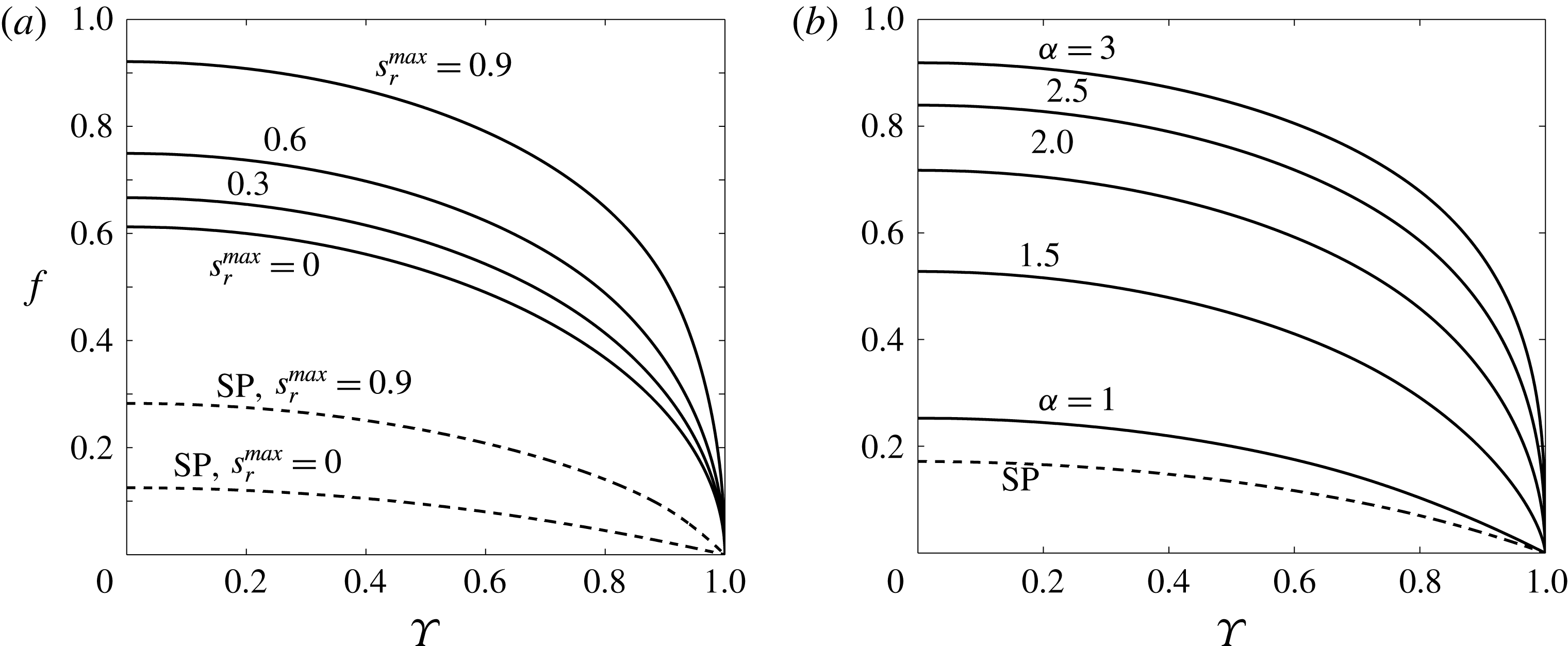
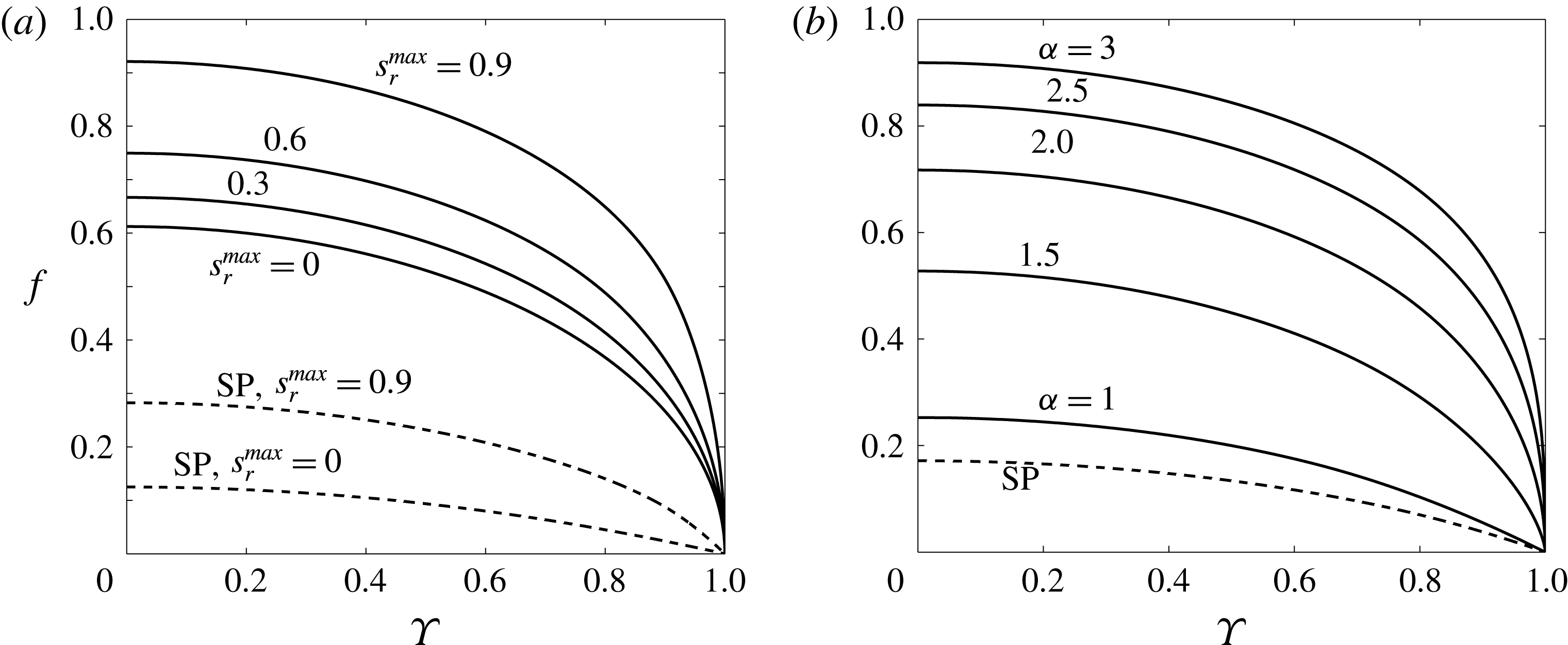
Scaled self-similar height profiles of a two-phase gravity current spreading in the long-time limit for (a) different values of the trapping fraction
 $s_{r}^{\mathit{max}}=0,0.3,0.6$
and 0.9, with fixed
 $\unicode[STIX]{x1D6FC}=2$
and (b) different relative permeability curves for
 $\unicode[STIX]{x1D6FC}=1,1.5,2,2.5$
and 3 with fixed
 $s_{r}^{\mathit{max}}=0.5$
. The profile at the nose of all the currents is described by (3.13). Equivalent results for the uniform-saturation, single-phase model (SP) are plotted by the black dashed lines (Kochina et al.
Reference Kochina, Mikhailov and Filinov1983; Lyle et al.
Reference Lyle, Huppert, Hallworth, Bickle and Chadwick2005).
3.1.2 Effect of altering the trapping fraction (
$s_{r}^{\mathit{max}}$
) and relative permeability curves (
$\unicode[STIX]{x1D6FC}$
)


Here we use the similarity solution to explore how certain empirical properties of the multiple phases and porous medium affect the shape and propagation rate of the gravity current.
The primary two-phase phenomena that affect the self-similar spreading of the finite-release gravity current are the trapping fraction,
 $s_{r}^{\mathit{max}}$
, which determines the rate at which fluid is left behind the current, and the relative permeability, characterised by
 $\unicode[STIX]{x1D6FC}$
, which determines the sensitivity of the flux to variations in saturation. We compare results in the following analysis to the constant-saturation model by Kochina et al. (Reference Kochina, Mikhailov and Filinov1983), where the constant trapping fraction
 $s_{r}^{\mathit{max}}$
also affects the self-similar spreading, but where the relative permeability, like the saturation, is constant and uniform in both advancing and receding parts of the current.
The spreading exponent
 $\unicode[STIX]{x1D6FD}$
is plotted as a function of
 $c_{D}/c_{I}=1-s_{r}^{\mathit{max}}$
in figure 4(b) for fixed trapping fraction
 $s_{r}^{\mathit{max}}$
and for five relative permeability curves (
 $\unicode[STIX]{x1D6FC}=1,1.5,2,2.5$
and 3). The corresponding propagation rate for a constant-saturation model found by Kochina et al. (Reference Kochina, Mikhailov and Filinov1983) is plotted using a black dashed curve. We see that the values of
 $\unicode[STIX]{x1D6FD}$
when
 $\unicode[STIX]{x1D6FC}=2$
correspond exactly to the constant-saturation case (Kochina et al.
Reference Kochina, Mikhailov and Filinov1983) because at this value in the long-time limit, the permeability and porosity are balanced in such a way that their coaction is similar to the single-phase case, as expressed in the scaling (2.25a
). In all cases, the value of
 $\unicode[STIX]{x1D6FD}$
is given by (3.15a
) when
 $s_{r}^{\mathit{max}}=0$
and decreases as the proportion of trapped fluid increases. The shape of the
 $\unicode[STIX]{x1D6FD}(s_{r}^{\mathit{max}})$
curves for different values of
 $\unicode[STIX]{x1D6FC}$
are similar, indicating that the effects of trapping and relative permeability are approximately independent.
The height profiles for two-phase gravity currents in the long-time limit are plotted for a selection of values of
 $s_{r}^{\mathit{max}}$
with fixed
 $\unicode[STIX]{x1D6FC}=2$
in figure 5(a). The thickening self-similar profile with increased trapping fraction is qualitatively similar to the constant-saturation case (Kochina et al.
Reference Kochina, Mikhailov and Filinov1983), plotted with dashed curves for
 $s_{r}^{\mathit{max}}=0$
and 0.9 in figure 5(a), although the nose shape is more rounded. The effect of relative permeability on the shape of the nose, as expressed by (3.13), is demonstrated in figure 5(b) for a selection of
 $\unicode[STIX]{x1D6FC}$
with fixed
 $s_{r}^{\mathit{max}}=0.5$
. The profile is linear for
 $\unicode[STIX]{x1D6FC}=1$
, as for the constant-saturation current plotted with a dashed curve, and becomes more rounded as
 $\unicode[STIX]{x1D6FC}$
increases. This is due to the need for greater height gradients to drive the fluid flux at the front where saturations and therefore relative permeabilities are smaller for higher
 $\unicode[STIX]{x1D6FC}$
, as observed for two-phase, constant-flux gravity currents (Golding et al.
Reference Golding, Neufeld, Hesse and Huppert2011).
3.2 Linear trapping: numerical solutions
In order to verify the self-similar solution in the long-time limit, in this subsection we numerically solve (2.30)–(2.32), with boundary conditions (2.33)–(2.35), while continuing to use the linear trapping model. We set
 $\unicode[STIX]{x1D6EC}_{D}=\unicode[STIX]{x1D6EC}_{I}=\unicode[STIX]{x1D6EC}$
and
 $\unicode[STIX]{x1D6FC}_{D}=\unicode[STIX]{x1D6FC}_{I}=\unicode[STIX]{x1D6FC}$
, so that hysteresis in the capillary pressure curves and saturation distributions in the two regions is introduced wherever either, or both of,
 $\unicode[STIX]{x1D6FF}>1$
and
 $s_{r}^{\mathit{max}}>0$
. We set
 $\unicode[STIX]{x1D6FF}=1.4$
in all our calculations, in order to represent a realistic porous medium (Gerhard & Kueper Reference Gerhard and Kueper2003). Consequently, the similarity solutions derived in § 3.1 are valid here only in the very long-time limit
 $\unicode[STIX]{x1D6EC}Bh\ll \unicode[STIX]{x1D6EC}Bh_{\mathit{max}}\ll 1$
. We specify the initial volume and profile of fluid between
 $r=[0,1]$
to be
 $$\begin{eqnarray}h(r,t=0)=h_{0}(1-r)^{1/2},\end{eqnarray}$$
where
 $h_{0}$
is a constant calculated for a set of parameters to ensure, using (2.35), that the dimensionless volume of fluid is 1.
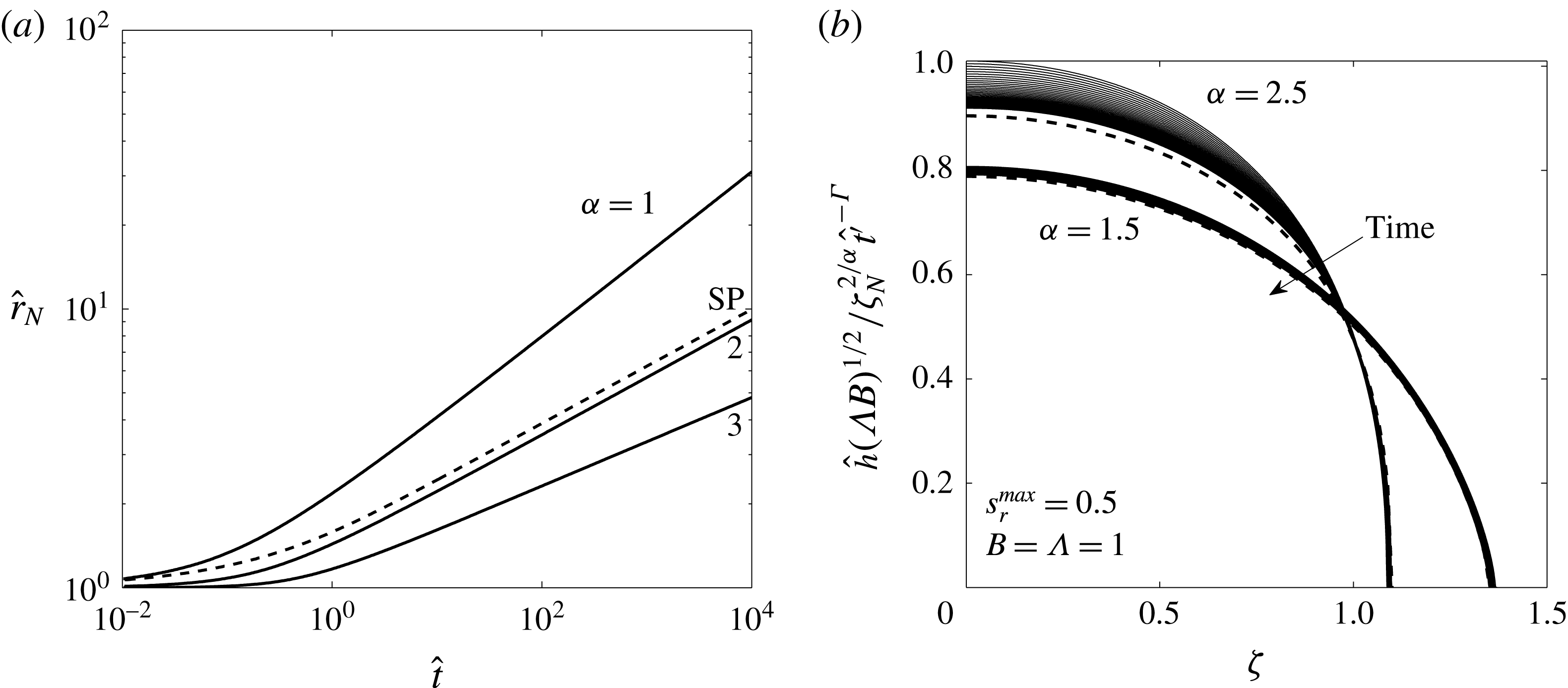
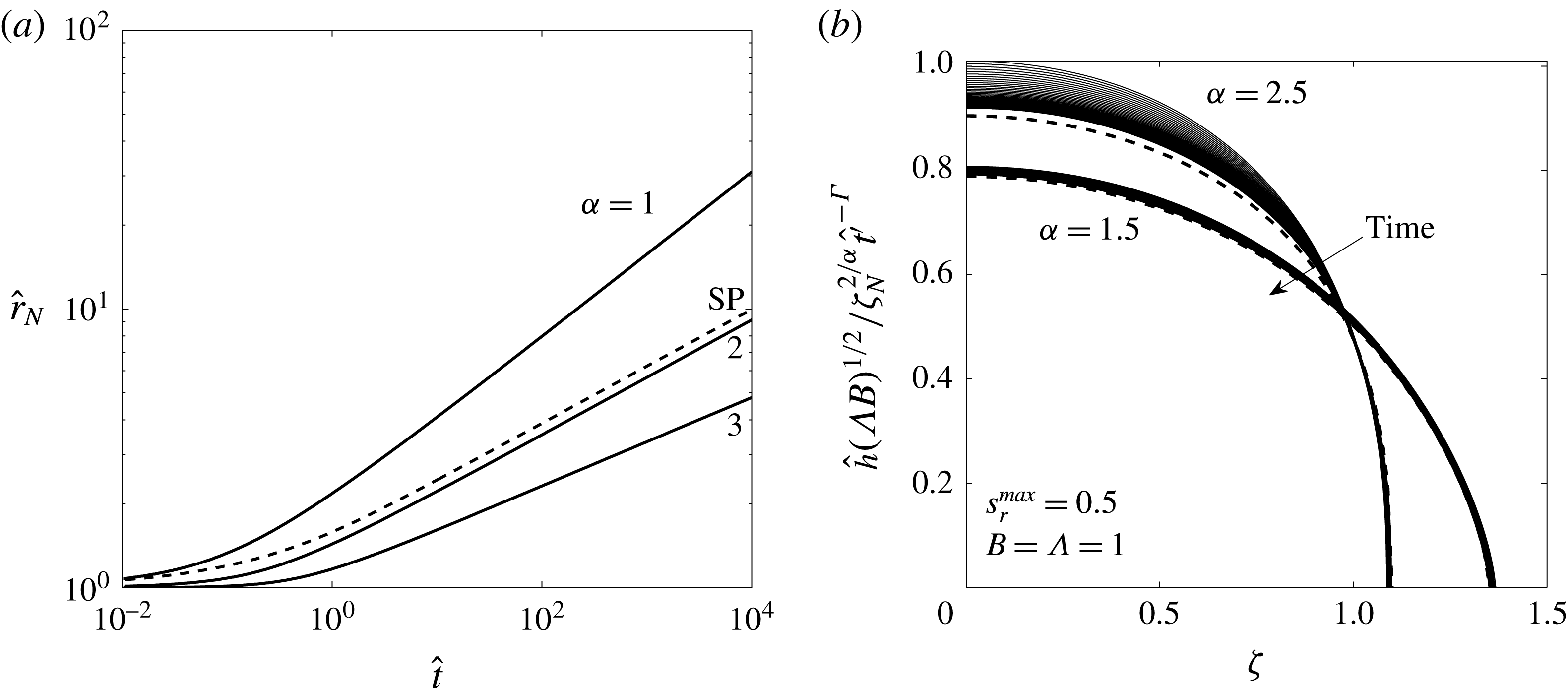
In figures 6(a) and 6(b), the radius and height profiles are plotted in terms of the dimensionless variables defined in § 2.6 for initially moderate capillary forces
 $\unicode[STIX]{x1D6EC}=B=1$
, for which
 $h_{0}=16.04$
. The radius is plotted for
 $\unicode[STIX]{x1D6FC}=1,2$
and 3, and we see that for each current, the radius increases according to the self-similar power law after approximately
 $\hat{t}\approx 10$
. The power of time,
 $\unicode[STIX]{x1D6FD}$
, can be correctly predetermined by the similarity solution and the values obtained from the numerical solutions in figure 6(a) are plotted using
 $\times$
markers in figure 4(b) for both the case
 $s_{r}^{\mathit{max}}=0.5$
here and also
 $s_{r}^{\mathit{max}}=0.1$
. The results indicate strong agreement between the numerical results and the theoretical similarity solution in the long-time limit. The radius of a single-phase, constant-saturation current is indicated by the dashed curve, where the fluid was initially contained within a flat-topped cylindrical volume for numerical reasons, which explains the slightly different behaviour at early times. The difference in spreading behaviour of the two-phase current compared to the single-phase current separated by
 $\unicode[STIX]{x1D6FC}=2$
is clearly visible. When
 $\unicode[STIX]{x1D6FC}=2$
, the single-phase current spreads faster due to a larger value of the similarity variable at the nose,
 $\unicode[STIX]{x1D701}_{N}$
, which can only be determined numerically.
Numerical solutions of a two-phase gravity current to validate the similarity solution in the long-time limit with a linear trapping relation,
 $s_{r}^{\mathit{max}}=0.5$
, for initially moderate capillary forces
 $B=\unicode[STIX]{x1D6EC}=1$
, and hysteresis introduced by
 $\unicode[STIX]{x1D6FF}=1.4$
. (a) Radius plotted against time for a two-phase current (solid curves) with
 $\unicode[STIX]{x1D6FC}=1,2$
and 3, where the initial residual relation is linear, defined by (2.11). A single-phase radius is plotted for comparison (dashed curve), and a comparison between the predicted and simulated power-law behaviour is shown in figure 4(b). (b) Numerical solutions (solid) and similarity solutions (dashed) for the height profile of the current
 $h$
against similarity variable
 $\unicode[STIX]{x1D701}$
, where
 $\unicode[STIX]{x1D701}_{N}$
is determined by the numerical simulations, for
 $\unicode[STIX]{x1D6FC}=1.5$
and 2.5. A number of numerical solutions are plotted for each case, corresponding to logarithmically spaced time horizons, and demonstrate the tendency towards the similarity shape.
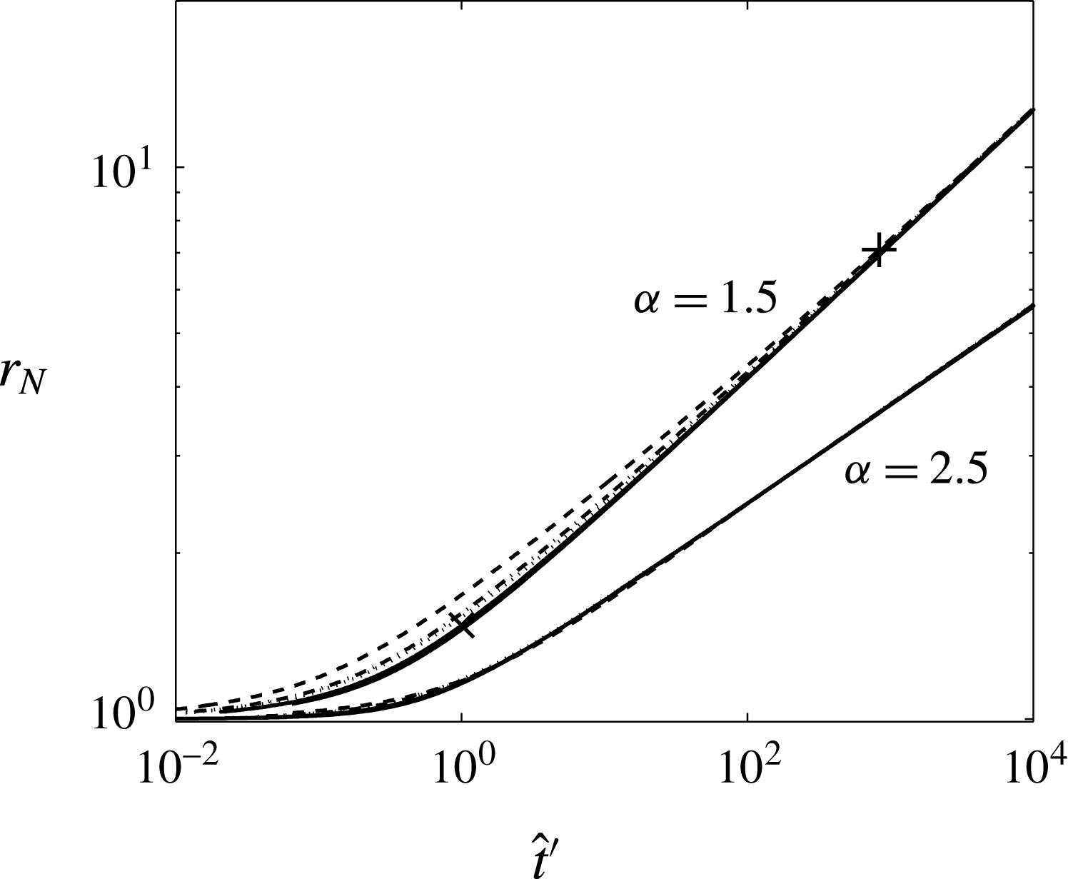
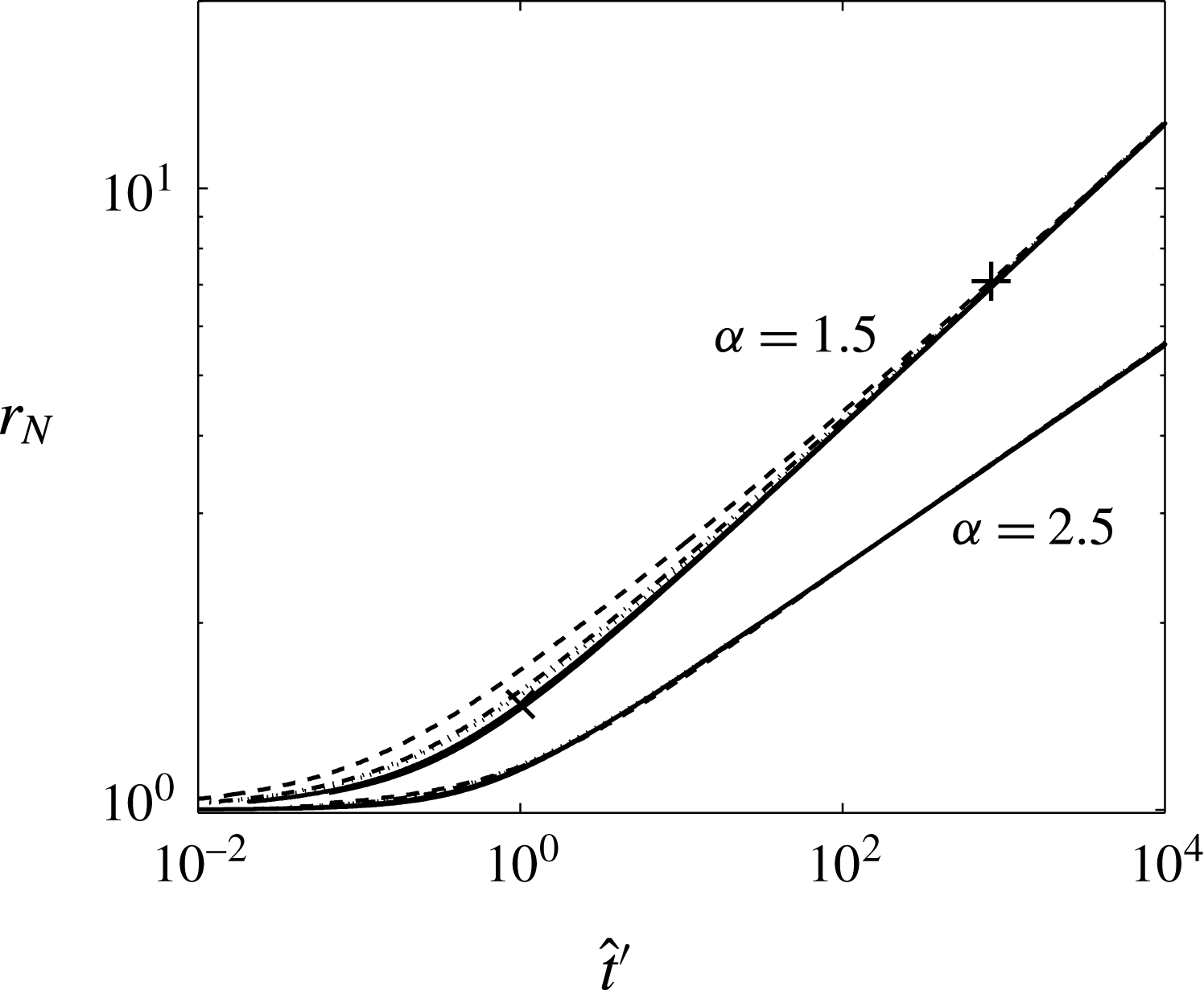
Radius plotted against scaled time, equation (3.8), for
 $\unicode[STIX]{x1D6FF}=1.4$
and linear trapping with
 $s_{r}^{\mathit{max}}=0.5$
. For each value of
 $\unicode[STIX]{x1D6FC}=1.5$
and 2.5, we plot the following curves as we vary the initial magnitude of capillary forces: (i) initially very strong capillary forces
 $B=\unicode[STIX]{x1D6EC}=0.1$
(solid curves); (ii) moderate capillary forces
 $B=\unicode[STIX]{x1D6EC}=1$
(solid); (iii) initially weak capillary forces
 $B=\unicode[STIX]{x1D6EC}=10$
(dashed); (iv) moderate gravity compared to capillarity but little variation in pore sizes
 $B=1$
,
 $\unicode[STIX]{x1D6EC}=10$
(dotted) and (v) weak gravity compared to capillarity but larger variation in pore sizes
 $B=10$
,
 $\unicode[STIX]{x1D6EC}=1$
(dash-dotted curves). Many of the curves are indistinguishable from others with the same
 $\unicode[STIX]{x1D6FC}$
because of the successful scaling.
Height profiles obtained numerically are plotted in figure 6(b) for logarithmically spaced snapshots of time between
 $\hat{t}=10$
and
 $10^{5}$
, for
 $\unicode[STIX]{x1D6FC}=1.5$
and 2.5 (solid curves). The height and radial extent are scaled according to (3.7a–c
), where
 $\unicode[STIX]{x1D701}_{N}$
is determined from the numerical calculations. The approach to a limiting, self-similar solution (dashed curves) is evident for both
 $\unicode[STIX]{x1D6FC}=1.5$
and 2.5.
The effect of the Bond number and pore-size distribution on the propagation rate of the current is to adjust the time scale of the spreading, as defined by (3.8), which depends only on the product
 $B\unicode[STIX]{x1D6EC}$
. Figure 7 demonstrates the effectiveness of this scaling, where the radial extent, plotted for various
 $B\unicode[STIX]{x1D6EC}$
, shows an excellent collapse of the data for both
 $\unicode[STIX]{x1D6FC}=1.5$
and
 $\unicode[STIX]{x1D6FC}=2.5$
. The approach to the late-time self-similar solution is faster when initial capillary forces are stronger, characterised by smaller
 $B\unicode[STIX]{x1D6EC}$
and also when relative permeability effects are magnified by the larger value of
 $\unicode[STIX]{x1D6FC}$
.
3.3 Land’s nonlinear trapping model
We now focus our attention on using Land’s nonlinear trapping model and discover our novel result, that the current no longer spreads in a self-similar manner in the long-time limit.
The behaviour of the trapping model plays a critical role in the dynamics of spreading, and the rates of capillary trapping. For linear trapping relationships a constant fraction of the receding current is trapped, leading to power-law spreading and a predicted, infinite long-time extent. Here we show that the most commonly used trapping model, Land’s model, which defines an empirical, nonlinear relationship between initial and residual saturation, leads to the possibility of a finite runout distance and hence a much more effective mode of trapping. At low initial saturations the residual saturation behaves approximately quadratically, resulting in a trapping fraction which changes with time as the saturation decreases. Thus the gravity current remains dependent on the historical height information and the model must be solved numerically for all times. As in § 3.2, we set
 $\unicode[STIX]{x1D6EC}_{D}=\unicode[STIX]{x1D6EC}_{I}=\unicode[STIX]{x1D6EC}$
and
 $\unicode[STIX]{x1D6FC}_{D}=\unicode[STIX]{x1D6FC}_{I}=\unicode[STIX]{x1D6FC}$
for simplicity, but incorporate hysteresis with
 $\unicode[STIX]{x1D6FF}>1$
and
 $s_{r}^{\mathit{max}}>0$
.
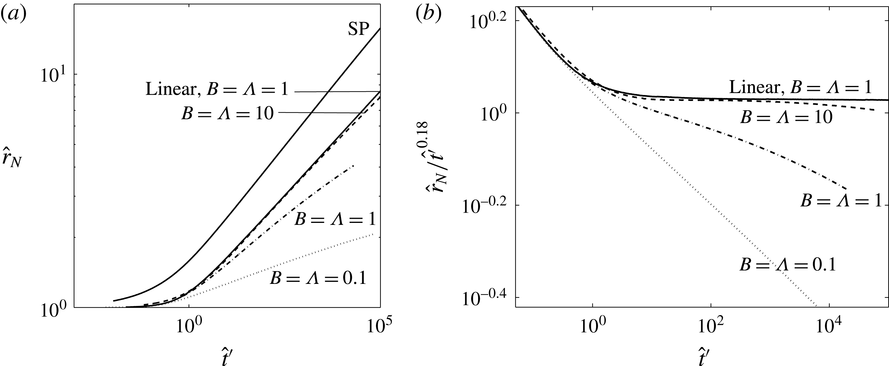
Figure 8(a) shows the dimensionless radial extent against time for several two-phase gravity currents using Land’s trapping model, along with an example of the two-phase radial extent using the linear trapping model. For comparison, the radius of the single-phase counterpart of these currents is also displayed. Relative permeability and hysteresis is the same for all curves drawn, characterised by
 $\unicode[STIX]{x1D6FC}=2.5$
,
 $s_{r}^{\mathit{max}}=0.5$
and
 $\unicode[STIX]{x1D6FF}=1.4$
. All the two-phase currents spread more slowly than the single-phase current with constant saturation because when
 $\unicode[STIX]{x1D6FC}=2.5>2$
, the relative permeability effects slow the current, despite the greater height gradients driving the flow, as discussed in § 3.1.2. Importantly, comparing the two-phase spreading using different models, we see that with Land’s trapping model, the currents decelerate over time for all values of
 $B=\unicode[STIX]{x1D6EC}=0.1,1$
and 10. This is in stark contrast to the current with a linear trapping model (solid, labelled curve) which spreads like
 $t^{0.18}$
when
 $\unicode[STIX]{x1D6FC}=2.5$
.
Numerical solution of the radial extent of a two-phase gravity current using Land’s trapping model with fixed parameters
 $\unicode[STIX]{x1D6FF}=1.4$
,
 $\unicode[STIX]{x1D6FC}=2.5$
and
 $s_{r}^{\mathit{max}}=0.5$
, where (a) the radius is plotted against scaled time,
 $\hat{t^{\prime }}$
, and (b) the radius is again plotted against
 $\hat{t^{\prime }}$
, but here is scaled by
 $\hat{t^{\prime }}^{0.18}$
, which is the self-similar power law found in the long-time limit for linear trapping (with
 $\unicode[STIX]{x1D6FC}=2.5$
). Results are displayed for strong, moderate and weak initial strengths of capillary forces, corresponding to
 $B=\unicode[STIX]{x1D6EC}=0.1,1$
and 10 respectively, as labelled next to the non-solid curves. The corresponding radial extent for a two-phase current with a linear trapping model and
 $B=\unicode[STIX]{x1D6EC}=1$
is also plotted in both figures (solid, labelled curve) and tends to the similarity solution derived in § 3.1, which is valid for all initial strengths of capillary forces when the trapping relation is linear (demonstrated in figure 7). The radius for an equivalent gravity current modelled using constant saturation (single phase), plotted in figure 8(a) (solid curve, labelled ‘SP’), also tends to a similarity solution (Kochina et al.
Reference Kochina, Mikhailov and Filinov1983).
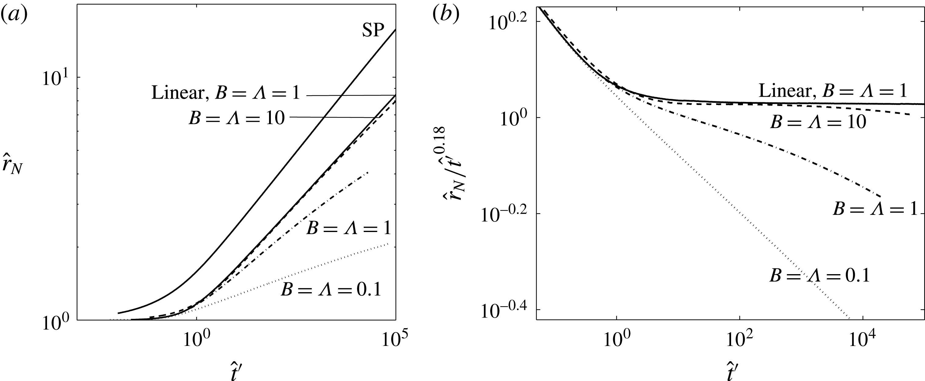
To further demonstrate the effect of using Land’s model instead of a linear trapping model, figure 8(b) displays the two-phase radius scaled by the long-time power law for the linear trapping model,
 $t^{0.18}$
. We see clearly that the gravity currents using Land’s trapping model decelerate with time relative to the linear model, because the saturation in the current decreases and the trapping fraction increases.
An important result is therefore that the propagation rate for all two-phase gravity currents with Land’s initial residual relation slows with time. This is because as the height of the current decreases, the initial saturations decrease, which leads to a higher proportion of fluid being trapped, i.e. a higher trapping fraction. It is useful to draw comparison with the similarity solution derived in § 3.1 for linear trapping which predicts the propagation rate in terms of the trapping fraction, in that case represented by
 $s_{r}^{\mathit{max}}$
, summarised in figure 4(b). There, as the trapping fraction increases, the propagation rate of the gravity current tends to 0. If we draw analogy to this for the radius of a gravity current with Land’s model, we would conclude that as the trapping fraction increases, tending to 1, the propagation rate tends to 0, i.e. the gravity current comes to a halt.
4 Residual trapping in a two-phase gravity current
In this section we consider the region of immobilised fluid left behind once the gravity current has receded, occupying the region
 $h<z<h_{max}$
in figure 1(a), and find that the proportion of fluid trapped here is always predicted to be greater when using Land’s model compared to the linear model.
Hitherto we have demonstrated the importance of the residual trapping model in determining the long-term spreading behaviour and characteristics of a two-phase gravity current, through both the diminishing volume of fluid in the current and the hysteresis in capillary pressure and relative permeability induced by trapped fluid. We now pay attention to the efficiency of residual trapping in different two-phase gravity currents and how it is affected by the trapping model, Bond number, pore-size distribution and relative permeability characteristics of the current and porous medium. In the case of a two-phase gravity current spreading beneath a caprock during the geological storage of
 $\text{CO}_{2}$
, an important quantity is the rate at which the released volume of
 $\text{CO}_{2}$
is likely to be residually trapped, and hence permanently immobilised. Another key question, particularly at preliminary stages of a
 $\text{CO}_{2}$
storage site, for example when assessing site suitability, is the ultimate extent to which the
 $\text{CO}_{2}$
may propagate.
We define an efficiency of trapping,
 $V_{r}$
, to be the proportion of the initial volume of fluid that is residually trapped. The initial volume of fluid in dimensionless terms is unity, and hence the efficiency of trapping is given by
 $$\begin{eqnarray}V_{r}=2\unicode[STIX]{x03C0}\int _{0}^{r_{b}}\int _{h}^{h_{\mathit{max}}}s_{r}(h_{\mathit{max}},z)\,\text{d}zr\,\text{d}r.\end{eqnarray}$$
This can be compared to the efficiency of storage used to investigate leakage from a
 $\text{CO}_{2}$
reservoir (Neufeld, Vella & Huppert Reference Neufeld, Vella and Huppert2009), as an estimate of the trade-off between storage and leakage.
The efficiency of trapping is influenced by three main factors. Firstly, the details of the trapping relationship, which are determined empirically in practice. We again illustrate the effects of the trapping relation by comparing results from the simple linear model and the more representative Land’s model, recalling that the trapping fraction (2.10) is constant in both the first and, trivially, the constant-saturation model, but varies in Land’s model. Second, the level of partial saturation of fluid within the current affects the efficiency of trapping via the trapping relation. The third main factor is the volume of porous medium which is contacted by the current as it spreads. This is often referred to in petroleum reservoir engineering as the sweep efficiency. The greater the sweep, which depends on the radius and height of the gravity current, the larger the volume of the reservoir that can be utilised for trapping. By definition of the two-phase saturation distribution, (2.6)–(2.9), fluid exists at lower saturations in two-phase gravity currents than in single-phase gravity currents, which leads to thicker currents. However, we have seen that the rate of spreading, and therefore radial and vertical extent, of the current depends on many two-phase parameters, such as the Bond number
 $B$
, pore-size distribution
 $\unicode[STIX]{x1D6EC}$
and relative permeability
 $\unicode[STIX]{x1D6FC}$
.
The efficiency of trapping as a function of the radius of the current for numerical simulations up to
 $\hat{t}=10^{4}$
, for fixed values of
 $\unicode[STIX]{x1D6FC}=1.5$
,
 $s_{r}^{\mathit{max}}=0.5$
and
 $\unicode[STIX]{x1D6FF}=1.4$
. The solid curves indicate the trapping efficiency using Land’s model and the dashed curve the efficiency using the linear trapping model. Different initial strengths of capillary forces are considered, as labelled with the value of
 $B=\unicode[STIX]{x1D6EC}$
. The equivalent curve for the constant-saturation (single-phase) model where the constant residual saturation is 0.5 is also plotted and labelled ‘SP’ (Kochina et al.
Reference Kochina, Mikhailov and Filinov1983).
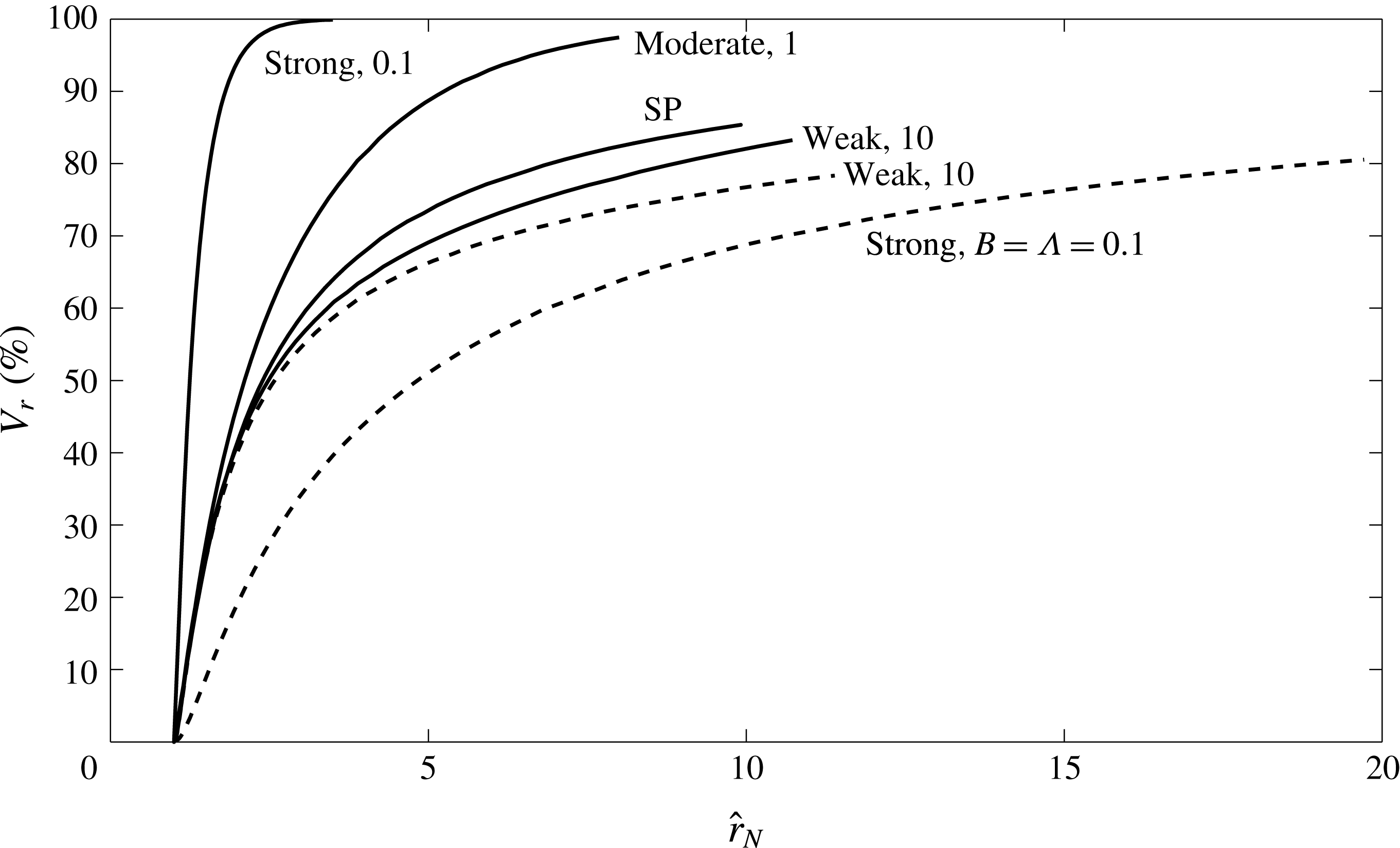
The trapping efficiency as a function of the radius of the gravity current is plotted for the linear and Land’s models in figure 9 using dashed and solid curves respectively. Various initial strengths of capillary forces are considered, labelled with their respective values of
 $B=\unicode[STIX]{x1D6EC}$
. The simulations are all run up to
 $\hat{t}=10^{4}$
for fixed
 $s_{r}^{\mathit{max}}=0.5$
and
 $\unicode[STIX]{x1D6FF}=1.4$
, and a common relative permeability constitutive relation,
 $\unicode[STIX]{x1D6FC}=1.5$
. The equivalent trapping efficiency for the constant-saturation (single-phase) model with the same value of the trapping parameter,
 $s_{r}^{\mathit{max}}=0.5$
, is also plotted for comparison with a solid line labelled ‘SP’ (Kochina et al.
Reference Kochina, Mikhailov and Filinov1983).
We see immediately that the trapping efficiency in two-phase gravity currents when using Land’s model is always greater than when using the linear model for a given radial extent. This is because Land’s model predicts a higher trapping fraction for a given maximum, or initial, saturation, than in the linear trapping model, where the trapping fraction remains constant as the current spreads and saturations decrease. Furthermore, the trapping efficiency increases with stronger initial capillary forces due to the higher trapping fractions at low saturations. It is worth noting that this characteristic of Land’s model is shared with many other constitutive initial residual relations (Pentland et al. Reference Pentland, Al-Mansoori, Iglauer, Bijeljic and Blunt2008).
The trapping efficiency for two-phase currents using the linear model is always lower than for the constant-saturation model with the same trapping fraction (Kochina et al.
Reference Kochina, Mikhailov and Filinov1983), despite having spread further (for the case displayed here,
 $\unicode[STIX]{x1D6FC}=1.5$
) and with a greater vertical sweep due to the partial saturations. This is because in both models the trapping fraction is equal to
 $s_{r}^{\mathit{max}}=0.5$
, and remains constant as the current spreads. In the two-phase current however, the decreasing partial saturation leads to an ever decreasing absolute volume being trapped per unit of porous medium as the current height recedes. Furthermore, in contrast to Land’s model, this means that the trapping efficiency decreases with stronger initial capillary forces.
For Land’s model and initially moderate and strong capillary forces, the trapping efficiency per unit radius is greater than the efficiency predicted by the single-phase model with its constant residual saturation and trapping fraction. The trapping efficiency for the Land’s model two-phase current is further enhanced by its increased vertical sweep, leading to a much higher volume of fluid being trapped in a smaller radius. In the case of very strong capillary forces when
 $B=\unicode[STIX]{x1D6EC}=0.1$
, nearly 100 % of the initial fluid is residually trapped by
 $\hat{t}=10^{4}$
and
 $\hat{r}_{N}\approx 3$
.
When capillary forces are initially weak,
 $B=\unicode[STIX]{x1D6EC}=10$
in our example, the trapping efficiency for two-phase currents using either trapping model is similar at early times to that for the constant-saturation model in which capillary forces remain negligible for all time. This is because the saturation is approximately unity in much of the two-phase currents and so both trapping models predict similar trapping fractions, equal to
 $s_{r}^{\mathit{max}}$
. However, for Land’s model, as the two-phase current spreads and the average maximum saturation decreases, we would expect the increasing trapping fraction to manifest in a trapping efficiency per unit radius rising above the single-phase level at later times.
The relative permeability for all scenarios considered here is parameterised by
 $\unicode[STIX]{x1D6FC}=1.5$
. We note that for larger values of
 $\unicode[STIX]{x1D6FC}$
, where relative permeability is more greatly inhibited at partial saturations, the behaviour in each case is characteristically similar. However, the trapping efficiency per unit radius is greater in all cases, presumably because of the greater sweep efficiency of these gravity currents.
5 Discussion and conclusions
We have derived a model for the evolution of a finite-volume, two-phase gravity current, which incorporates the key two-phase phenomena that arise when drainage and imbibition occur simultaneously in different regions of the current. Residual trapping of fluid during imbibition in receding regions of the current is described using an empirical trapping model, which determines the evolving saturation distribution there as a function of space and time. This is used to capture in a consistent way the end points in the hysteretic capillary pressure and relative permeability primary and secondary scanning curves. The resulting model encapsulates the key pore-scale capillary phenomena within specially defined saturation and flux functions which differ in the drainage and imbibition regions, whilst still resembling the traditional framework often used to describe gravity currents (see, for example, Huppert & Woods Reference Huppert and Woods1995). Thus two-phase gravity currents with trapping and hysteresis may be investigated at much lower computational costs than solving the full equations numerically.
We explained how the fundamental depth-integrated momentum conservation equation (2.14), could be combined with the empirical models for multiphase flow to define the saturation and flux functions (2.15)–(2.21), along with the no-flux boundary conditions, continuity of height and flux, and global conservation of mass, equations (2.22)–(2.24).
Using this model, we investigated how the behaviour of the current is affected by the saturation distribution of spreading fluid, governed by the Bond number and pore-size distribution, along with the constitutive relation between relative permeability and saturation and the extent of residual trapping. We paid particular attention to the importance of residual trapping because it underpins the hysteresis exhibited in both capillary pressure and relative permeability relations, and consequently the fundamental behaviour of two-phase gravity currents.
One of the key findings of our analysis is that when residual trapping occurs, the initial residual relation, or trapping model, is critical in determining the long-time behaviour of the two-phase gravity current. If the trapping relation is given by the commonly used Land’s model, the trapping fraction increases as saturation decreases with time and the gravity currents slow down, which we demonstrated by solving the full governing equations numerically. Furthermore, at very low saturations the trapping fraction tends to unity and therefore, if our assumptions remain valid, the model suggests that the two-phase gravity current will slow down and eventually stop.
In contrast, when the trapping fraction is constant at low saturations, such as for the linear model, the gravity current tends to a self-similar solution of the second kind in the long-time limit, with saturation proportional to the current height. The gravity current therefore spreads indefinitely, constantly slowing down, akin to the uniform-saturation solution derived by Kochina et al. (Reference Kochina, Mikhailov and Filinov1983) and two-phase models by Van Dijke & Van der Zee (Reference Van Dijke and Van der Zee1997) and Bear & Ryzhik (Reference Bear and Ryzhik1998). In these cases, we found that the long-term behaviour is determined not only by the trapping fraction, but also by the balance between the steeper height gradients and reduced permeability caused by partial saturation. The explicit form of motion is divided by the critical value
 $\unicode[STIX]{x1D6FC}=\unicode[STIX]{x1D6FC}_{c}=2$
, where
 $\unicode[STIX]{x1D6FC}$
parameterises the empirical relation between relative permeability and saturation. When
 $\unicode[STIX]{x1D6FC}>\unicode[STIX]{x1D6FC}_{c}$
, the relative permeability is significantly reduced at low saturations and this leads to the two-phase gravity current spreading more slowly than an equivalent single-phase counterpart. When
 $\unicode[STIX]{x1D6FC}<\unicode[STIX]{x1D6FC}_{c}$
the increased gradient of the height profile drives a larger flux of fluid in the current, and hence the two-phase gravity current spreads more quickly than a single-phase counterpart. The power law of time for the radius of the current can be estimated reasonably well from the results for the simpler, uniform-saturation model, with a simple multiplicative scaling factor to account for the effects of relative permeability. However, the height profile differs from the single-phase current by being larger, with a steeper profile at the front, as has been found for constant-flux two-phase gravity currents (Golding et al.
Reference Golding, Neufeld, Hesse and Huppert2011; Nordbotten & Dahle Reference Nordbotten and Dahle2011). The behaviour of the current when capillary forces are strong depends only on the product of the Bond number and the pore-size distribution,
 $B\unicode[STIX]{x1D6EC}$
. The behaviour of the gravity current in this limit also loses its dependence on the ratio of terminal to entry capillary pressures,
 $\unicode[STIX]{x1D6FF}$
, at very late times when
 $Bh_{\mathit{max}}\ll 1$
for the majority of the current, i.e. when the maximum saturation profile is proportional to
 $h_{\mathit{max}}$
. These similarity solutions provide useful, easily computable bounds and tests for more complex scenarios which require numerical solution of the governing equations.
The effects of residual trapping have been captured consistently and completely in this model, both in terms of the hysteresis of capillary pressure and relative permeability relations, and the fluid left behind as the current spreads. We find that for two-phase currents with linear trapping and a constant trapping fraction, equivalent to that in a single-phase current, fluid is immobilised by residual trapping at a slower rate than in a single-phase current because of the partial saturations. However, the trapping fraction in most realistic initial residual constitutive relations is higher when the initial saturation is small, compared to when the initial saturation is 1 (Pentland et al. Reference Pentland, Al-Mansoori, Iglauer, Bijeljic and Blunt2008). In these cases, the trapping efficiency of two-phase gravity currents is much greater than for the linear trapping model. The efficiency increases with increasing strength of capillary forces because of the greater vertical sweep and fluid spreading at lower saturations.
This dependence on the trapping model highlights the importance of resolving the saturation distribution and its evolution within a two-phase gravity current. In the context of the geological storage of
 $\text{CO}_{2}$
, the sweep of a two-phase gravity current is much larger than that of a single-phase current, regardless of the shape of the initial residual relation. This means that the
 $\text{CO}_{2}$
has greater contact with both the brine and the rock, which is beneficial for other trapping processes to take place such as dissolution or mineral trapping. However, when considered alone the implications of a vertical saturation distribution and nonlinear trapping model (such as Land’s) is to impose a finite lateral extent for buoyant
 $\text{CO}_{2}$
gravity currents. This prediction, particularly when tested against field trials, would provide a strong additional constraint on the total possible contact area of sequestered
 $\text{CO}_{2}$
, thereby enabling geological
 $\text{CO}_{2}$
storage to be licensed in a wider variety of geological strata due to the efficacy of capillary trapping in ultimately immobilising buoyant
 $\text{CO}_{2}$
. Finally, it should be noted that the results of this study strictly apply to unconfined aquifers where the vertical extent of the aquifer far exceeds the height of the current (as is likely the case at Sleipner, for example, Cowton et al.
Reference Cowton, Neufeld, White, Bickle, White and Chadwick2016). While previous work has examined the transitions from confined to unconfined flow (Hesse et al.
Reference Hesse, Tchelepi, Cantwell and Orr2007), and the trapping rates in sloping aquifers (Hesse, Orr Jr & Tchelepi Reference Hesse, Orr and Tchelepi2008), further work is necessary to examine the influence of the flow of ambient water on trapping in multiphase current in more confined settings, as could be the case for many
 $\text{CO}_{2}$
injection projects.
Acknowledgements
The research of M.J.G. is funded by the EPSRC. H.E.H. is partially supported by a Wolfson Royal Society merit award and a Leverhulme Emeritus Fellowship. J.A.N. is supported by a Royal Society University Research Fellowship. We are all grateful for this support.