1 Introduction
Granular flows abound in the natural environment (rock avalanches, debris flows, landslides) and are met in innumerable industrial and agricultural applications concerning the transport and processing of cereals, ores, sand or any other material consisting of grains (Jaeger, Nagel & Behringer Reference Jaeger, Nagel and Behringer1996; Jakob & Hungr Reference Jakob and Hungr2005; Aranson & Tsimring Reference Aranson and Tsimring2006; Pudasaini & Hutter Reference Pudasaini and Hutter2007; Andreotti, Forterre & Pouliquen Reference Andreotti, Forterre and Pouliquen2013; Takahashi Reference Takahashi2014). These flows have attracted a lot of attention during the past three decades, not only because they have a multitude of practical applications but also because of the fundamental insights that are gained from them and the beauty of the physics involved. One of the key questions is to what extent granular flows admit a hydrodynamic-like description (Kadanoff Reference Kadanoff1999) and, although in its full generality this question is still open, the hydrodynamic approach has already been used with great success in a variety of special cases (Savage & Hutter Reference Savage and Hutter1989; Eggers Reference Eggers1999; Pouliquen & Forterre Reference Pouliquen and Forterre2002; Eshuis et al. Reference Eshuis, van der Weele, van der Meer and Lohse2005, Reference Eshuis, van der Meer, Alam, van Gerner, van der Weele and Lohse2010; Johnson & Gray Reference Johnson and Gray2011; Razis et al. Reference Razis, Edwards, Gray and van der Weele2014). In particular, for the case of granular chute flow, a shallow water description in the spirit of the Saint-Venant equations, augmented by novel constitutive relations reflecting the characteristic nature of the granular fluid, has given very satisfactory results.
In the late 1980s, Savage & Hutter (Reference Savage and Hutter1989) were among the first to formulate this approach, which is based on the continuity equation and momentum balance, from which the thickness of the flowing sheet
 $h(x,t)$
and the depth-averaged velocity
 $\bar{u}(x,t)$
along the chute can be determined. Around the turn of the century Pouliquen & Forterre (Reference Pouliquen and Forterre2002) added an important refinement to this model by giving an accurate expression for the friction force exerted on the sheet by the chute. In 2014 the set of equations was completed – and cured from ill posedness in the relevant regime of inclination angles for which steady uniform flow is possible – by Gray & Edwards (Reference Gray and Edwards2014), who introduced a novel viscous-like term into the momentum balance, derived from first principles using
 $\unicode[STIX]{x1D707}(I)$
-rheology (GDR-MiDi 2004) and depth integrating the in-plane stresses in the granular sheet.
This approach has proven to be able to capture various important waveforms of granular chute flow. The question that arises is: does every wave solution of the Saint-Venant equations for water have its counterpart in flowing sand? Up to now, such counterparts have been found for three of the four major ‘Saint-Venant’ waveforms:
(i) Roll waves, which are a common phenomenon in water spillways and irrigation channels (Dressler Reference Dressler1949; Needham & Merkin Reference Needham and Merkin1984) when the Froude number
 $Fr=\bar{u}/\sqrt{gh\cos \unicode[STIX]{x1D701}}$
exceeds the critical value of
 $2$
. Here
 $h$
and
 $\bar{u}$
denote the height and depth-averaged velocity of the flow,
 $\unicode[STIX]{x1D701}$
the inclination angle of the channel and
 $g$
the gravitational acceleration. Recently, roll waves have also been identified in granular chute flow (Gray & Edwards Reference Gray and Edwards2014; Razis et al.
Reference Razis, Edwards, Gray and van der Weele2014), with the subtle difference that in this case the threshold value of
 $Fr$
happens to be
 $2/3$
.
(ii) Stationary hydraulic jumps, which often occur in waterways behind sluice gates (Rayleigh Reference Rayleigh1914; Rouse Reference Rouse1946) where a shallow, fast supercritical flow (
 $Fr>1$
) suddenly becomes thicker and slower, such that the Froude number drops below unity, meaning that the flow turns subcritical (
 $Fr<1$
). The same phenomenon appears in granular flows (Boudet et al.
Reference Boudet, Amarouchene, Bonnier and Kellay2007; Gray & Cui Reference Gray and Cui2007; Johnson & Gray Reference Johnson and Gray2011; Mejean, Faug & Einav Reference Mejean, Faug and Einav2017a
,Reference Mejean, Faug, Einav, Radjai, Nezamabadi, Luding and Delenne
b
; Viroulet et al.
Reference Viroulet, Baker, Edwards, Johnson, Gjaltema, Clavel and Gray2017) and, just as in water, it takes place at
 $Fr=1$
.
(iii) Travelling hydraulic jumps. These always propagate upstream, since in the other direction they would be expansion waves with an ever flattening structure (Stoker Reference Stoker1958; Whitham Reference Whitham1974; Fowler Reference Fowler2011); they are also found in granular chute flow (Gray, Tai & Noelle Reference Gray, Tai and Noelle2003), at
 $Fr=1$
in the co-moving frame. These upstream travelling jumps can be viewed as non-undular bores. In nature, bores often exhibit undulations on the upper flank of the jump profile, such as the well-known tidal bore on the river Severn in the United Kingdom and the ‘mascaret’ on the Seine in France (Bonneton et al.
Reference Bonneton, Filippini, Arpaia, Bonneton and Ricchiuto2016; Rousseaux et al.
Reference Rousseaux, Mougenot, Chatellier, David and Calluaud2016). A dispersive term is needed to model these undulations (Peregrine Reference Peregrine1966; Benjamin, Bona & Mahony Reference Benjamin, Bona and Mahony1972; Whitham Reference Whitham1974; Fowler Reference Fowler2011) and hence, since dispersion is absent from the Saint-Venant equations, this feature of bores is not captured by the original Saint-Venant approach.
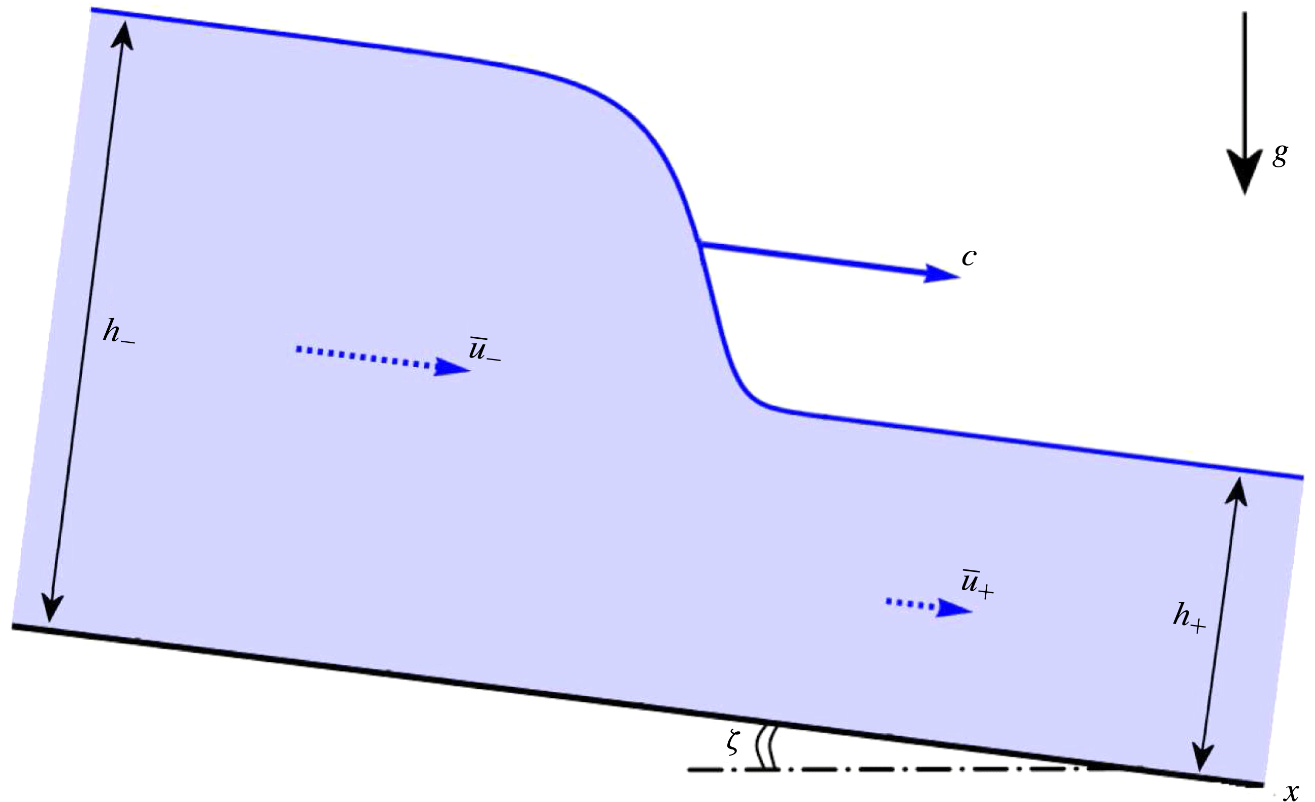
Monoclinal wave in a water channel, obtained by numerical integration of the Saint-Venant equations for water, see e.g. Whitham (Reference Whitham1974), Fowler (Reference Fowler2011): a relatively deep region of uniform height
 $h_{-}$
and depth-averaged velocity
 $\bar{u}_{-}$
overtakes a shallower and slower region of height
 $h_{+}$
and velocity
 $\bar{u}_{+}$
. A wave like this is generated for instance when a sluice gate, first opened only partially such as to permit the passage of a thin sheet of water (height
 $h_{+}$
), is subsequently opened further to let through a sheet of greater height
 $h_{-}$
. The travelling monoclinal wave is the stable shock structure connecting these two regions, preserving its shape thanks to a non-trivial balance of all forces at work. The wave propagates with a wave speed
 $c$
that exceeds the velocities of both plateaus, i.e.
 $c>\bar{u}_{-}>\bar{u}_{+}$
. The inclination of the channel has been explicitly depicted here; in all of the following figures the
 $x$
-axis will be drawn horizontally, with the inclination angle
 $\unicode[STIX]{x1D701}$
being silently understood.

Only the fourth major waveform, i.e.
(iv) Monoclinal waves, with both plateaus flowing, have until now not been reported in a granular context. In water channels they are known to occur for
 $Fr<2$
when a high-level region flows downstream over a region of smaller depth, as depicted in figure 1 (Moots & Mavis Reference Moots and Mavis1938; Whitham Reference Whitham1974; Ferrick Reference Ferrick2005; Shome & Steffler Reference Shome and Steffler2006; Fowler Reference Fowler2011). In this study, we show that the same type of wave is possible in granular chute flows when the Froude number is below
 $Fr=2/3$
(in the laboratory frame). The reason why it cannot exist for larger Froude numbers is the Kapitza instability (Kapitza & Kapitza Reference Kapitza and Kapitza1949): for
 $Fr>2/3$
a uniformly flowing granular sheet ceases to be stable and spontaneously breaks into a series of ripples that eventually ripen into roll waves (Forterre & Pouliquen Reference Forterre and Pouliquen2003; Gray & Edwards Reference Gray and Edwards2014; Razis et al.
Reference Razis, Edwards, Gray and van der Weele2014).
As an interesting aside, we note that a mechanical analogue of the monoclinal wave seen in figure 1 may be found in the celebrated antikink solution propagating along an array of pendulums coupled via torsion springs, modelled by the sine-Gordon equation (see e.g. Drazin & Johnson Reference Drazin and Johnson1988). Also this antikink is a nonlinear wave connecting two plateau values (differing by
 $2\unicode[STIX]{x03C0}$
radians) in a smooth, monotonically descending fashion.
The paper is organized as follows. In § 2 we introduce the governing equations, being the mass and momentum balance respectively, with appropriate constitutive relations for the friction and the viscous-like term. By numerically solving these equations we show that a monoclinal wave is (under the right circumstances) a perfectly feasible, stable travelling wave solution. We also show that it can be somewhat difficult to recognize this type of wave in practice, due to the fact that the longitudinal length scale of the wave is several orders of magnitude larger than its amplitude
 $\unicode[STIX]{x0394}h=h_{-}-h_{+}$
, explaining its elusiveness in experiments so far. In § 3 we present a travelling wave analysis, give the differential equation that governs the exact shape of the granular monoclinal wave and also discuss its close relation with avalanche fronts propagating on an empty chute. One of the things transpiring from this analysis is that the influence of the viscous-like term is restricted to a small portion of the monoclinal wave, and therefore in § 4 the inviscid limit is discussed in some extra detail. In § 5 we describe the balance of forces responsible for the stability of the monoclinal wave. Finally, in § 6 we summarize our findings and give the window of parameter values where granular monoclinal waves are expected to be found, which we hope will serve as a roadmap for future experiments.
2 Setting the stage
2.1 The governing equations
Granular chute flow, in the spirit of the shallow water approximation for normal fluids, is fully described in terms of the height of the granular sheet,
 $h(x,t)$
, and the depth-averaged velocity
 $\bar{u}(x,t)$
. In this description, the velocity profile is taken to depend only on
 $x$
and
 $t$
. The variations in the cross-wise direction (
 $y$
) are ignored and the variations over depth (
 $z$
) are averaged out:
 $$\begin{eqnarray}\bar{u}(x,t)=\frac{1}{h(x,t)}\int _{0}^{h(x,t)}u(x,z,t)\,\text{d}z.\end{eqnarray}$$
Mathematically, the depth-averaging process (one of the hallmarks of the Saint-Venant approach) is possible for any velocity profile and does not assume anything about the
 $z$
-dependence of
 $u(x,z,t)$
. A wide variety of velocity profiles can be met in granular flows (Savage & Hutter Reference Savage and Hutter1989; Forterre & Pouliquen Reference Forterre and Pouliquen2003; Forterre Reference Forterre2006; Gray & Ancey Reference Gray and Ancey2009; Gray & Kokelaar Reference Gray and Kokelaar2010), including granular plug flow, linear shear flow with or without basal slip and the celebrated Bagnold profile. In all these cases the depth averaging makes physical sense. This is especially evident for plug flow, which does not vary with
 $z$
, since in that case the depth-averaged velocity
 $\bar{u}(x,t)$
actually provides an exact representation.
The two fields
 $h(x,t)$
and
 $\bar{u}(x,t)$
are governed by a system of two coupled nonlinear differential equations (Gray & Edwards Reference Gray and Edwards2014; Razis et al.
Reference Razis, Edwards, Gray and van der Weele2014; Edwards & Gray Reference Edwards and Gray2015). The first one of these is the continuity equation, or mass balance, expressing the conservation of material along the chute:
 $$\begin{eqnarray}\frac{\unicode[STIX]{x2202}h}{\unicode[STIX]{x2202}t}+\frac{\unicode[STIX]{x2202}}{\unicode[STIX]{x2202}x}(h\bar{u})=0,\end{eqnarray}$$
and the second one is the so-called equation of motion, or momentum balance, which takes the following form:
 $$\begin{eqnarray}\displaystyle \frac{\unicode[STIX]{x2202}}{\unicode[STIX]{x2202}t}(h\bar{u})+\frac{\unicode[STIX]{x2202}}{\unicode[STIX]{x2202}x}(h\bar{u}^{2})=gh\sin \unicode[STIX]{x1D701}-\frac{\unicode[STIX]{x2202}}{\unicode[STIX]{x2202}x}\left(\frac{1}{2}gh^{2}\cos \unicode[STIX]{x1D701}\right)-\unicode[STIX]{x1D707}(h,\bar{u})gh\cos \unicode[STIX]{x1D701}+\frac{\unicode[STIX]{x2202}}{\unicode[STIX]{x2202}x}\left(\unicode[STIX]{x1D708}h^{3/2}\frac{\unicode[STIX]{x2202}\bar{u}}{\unicode[STIX]{x2202}x}\right). & & \displaystyle \nonumber\\ \displaystyle & & \displaystyle\end{eqnarray}$$
The continuity equation (2.2) states that, for any control volume along the chute, a net influx of material, given mathematically by
 $-\unicode[STIX]{x2202}_{x}(h\bar{u})$
, causes a change in height given by
 $\unicode[STIX]{x2202}_{t}h$
. Here we assume that the granular material has a constant density
 $\unicode[STIX]{x1D70C}$
, i.e. that it may be treated as an incompressible fluid. This has also been used in the momentum balance (2.3), which has been divided by
 $\unicode[STIX]{x1D70C}$
throughout. This latter balance states that the change of momentum of the material in the control volume, represented by the Stokesian derivative on the left-hand side, is equal to the sum of all forces acting on this volume. (We are talking about forces, but please note that the terms in (2.3) are not expressed in N but in
 $\text{m}^{2}~\text{s}^{-2}$
. This is because the momentum balance (force per unit volume) has been integrated over the depth (giving an extra dimension of length) and divided throughout by the constant density
 $\unicode[STIX]{x1D70C}$
(mass per unit volume). So ‘force’ in the present discussion actually stands for ‘depth-integrated force per unit volume divided by the density’.)
The contributing forces are, in the order in which they appear in the right-hand side of (2.3):
(i) The component of the gravitational force acting along the chute,
 $gh\sin \unicode[STIX]{x1D701}$
(with
 $\unicode[STIX]{x1D701}$
being the inclination angle of the chute).
(ii) The gradient of the depth-averaged pressure
 $-\unicode[STIX]{x2202}_{x}((1/2)gh^{2}\cos \unicode[STIX]{x1D701})$
, or equivalently
 $-g\cos \unicode[STIX]{x1D701}h\unicode[STIX]{x2202}_{x}h$
, due to variations in the height
 $h(x,t)$
assuming a standard hydrostatic pressure profile within the sheet.
(iii) The friction the granular sheet experiences from the chute,
 $-\unicode[STIX]{x1D707}(h,\bar{u})gh\cos \unicode[STIX]{x1D701}$
, which has the form of a (height- and velocity-dependent) friction coefficient
 $\unicode[STIX]{x1D707}(h,\bar{u})$
multiplied by the normal reaction force exerted on the granular material. Various expressions for the friction coefficient have been proposed in the literature (Savage & Hutter Reference Savage and Hutter1989; Daerr & Douady Reference Daerr and Douady1999; Pouliquen & Forterre Reference Pouliquen and Forterre2002). Of these, we will use the one first introduced by Pouliquen (Reference Pouliquen1999) and presented in the following form by Razis et al. (Reference Razis, Edwards, Gray and van der Weele2014), which gives a good description as long as the granular material is flowing in the fully dynamic regime (Pouliquen & Forterre Reference Pouliquen and Forterre2002):
 $$\begin{eqnarray}\unicode[STIX]{x1D707}(h,\bar{u})=\tan \unicode[STIX]{x1D701}_{1}+\frac{\tan \unicode[STIX]{x1D701}_{2}-\tan \unicode[STIX]{x1D701}_{1}}{1+\unicode[STIX]{x1D6FD}{\mathcal{L}}^{-1}\sqrt{g\cos \unicode[STIX]{x1D701}}h^{3/2}\bar{u}^{-1}},\end{eqnarray}$$
where
 $\unicode[STIX]{x1D701}_{1},\unicode[STIX]{x1D701}_{2},\unicode[STIX]{x1D6FD}$
and
 ${\mathcal{L}}$
are experimental parameters.
Here
 $\unicode[STIX]{x1D701}_{1}$
and
 $\unicode[STIX]{x1D701}_{2}$
denote the two inclination angles that delimit the interval in which uniform granular flows are observed. For
 $\unicode[STIX]{x1D701}<\unicode[STIX]{x1D701}_{1}$
the granular sheet remains immobile, whereas for
 $\unicode[STIX]{x1D701}>\unicode[STIX]{x1D701}_{2}$
the grains are swept downwards in an uncontrollable avalanche. For definiteness, we will choose
 $\unicode[STIX]{x1D701}_{1}=32.9^{\circ }$
(
 $\tan \unicode[STIX]{x1D701}_{1}=0.647$
) and
 $\unicode[STIX]{x1D701}_{2}=42.0^{\circ }$
(
 $\tan \unicode[STIX]{x1D701}_{2}=0.900$
), which are the values for the particular chute with the roughened surface that we used in a recent study on granular roll waves (Razis et al.
Reference Razis, Edwards, Gray and van der Weele2014).
The parameter
 $\unicode[STIX]{x1D6FD}$
is a dimensionless number having to do with the particles used, ranging from
 $0.136$
for smooth spherical particles (Pouliquen & Forterre Reference Pouliquen and Forterre2002) to approximately
 $0.65$
for rough carborundum particles (Gray & Edwards Reference Gray and Edwards2014; Razis et al.
Reference Razis, Edwards, Gray and van der Weele2014) and possibly even larger for other particles. In the present study we will take
 $\unicode[STIX]{x1D6FD}=0.5$
as a representative typical value. The parameter
 ${\mathcal{L}}$
is a length scale related to the thickness of the deposition layer which is left on the chute when a granular flow has passed over it and the inflow of new material is terminated; we will take a typical value of
 ${\mathcal{L}}=10^{-3}~\text{m}$
.
In practice, the parameters
 $\unicode[STIX]{x1D6FD}$
and
 ${\mathcal{L}}$
are extracted from empirical measurements:
 ${\mathcal{L}}$
is found by measuring the thickness of the deposit left behind by a uniform flow and, once
 ${\mathcal{L}}$
is known, the value of
 $\unicode[STIX]{x1D6FD}$
follows by measuring the depth-averaged velocity of a uniformly flowing granular sheet as a function of its thickness and fitting the data with (2.6) below. Thus, the parameters
 ${\mathcal{L}}$
and
 $\unicode[STIX]{x1D6FD}$
are not strictly independent of each other and the ‘typical’ values chosen above (
 ${\mathcal{L}}=10^{-3}~\text{m}$
,
 $\unicode[STIX]{x1D6FD}=0.50$
in combination with the given values of
 $\unicode[STIX]{x1D701}_{1}$
and
 $\unicode[STIX]{x1D701}_{2}$
) may possibly not correspond exactly to an existing experimental set-up. They are realistic, however, and – as we will see – quite adequate for demonstrating the physics of the granular monoclinal wave. In § 6, when we discuss the feasibility of detecting monoclinal waves in the lab, we will come back to this question and also consider two parameter sets that have been measured in actual experiments.
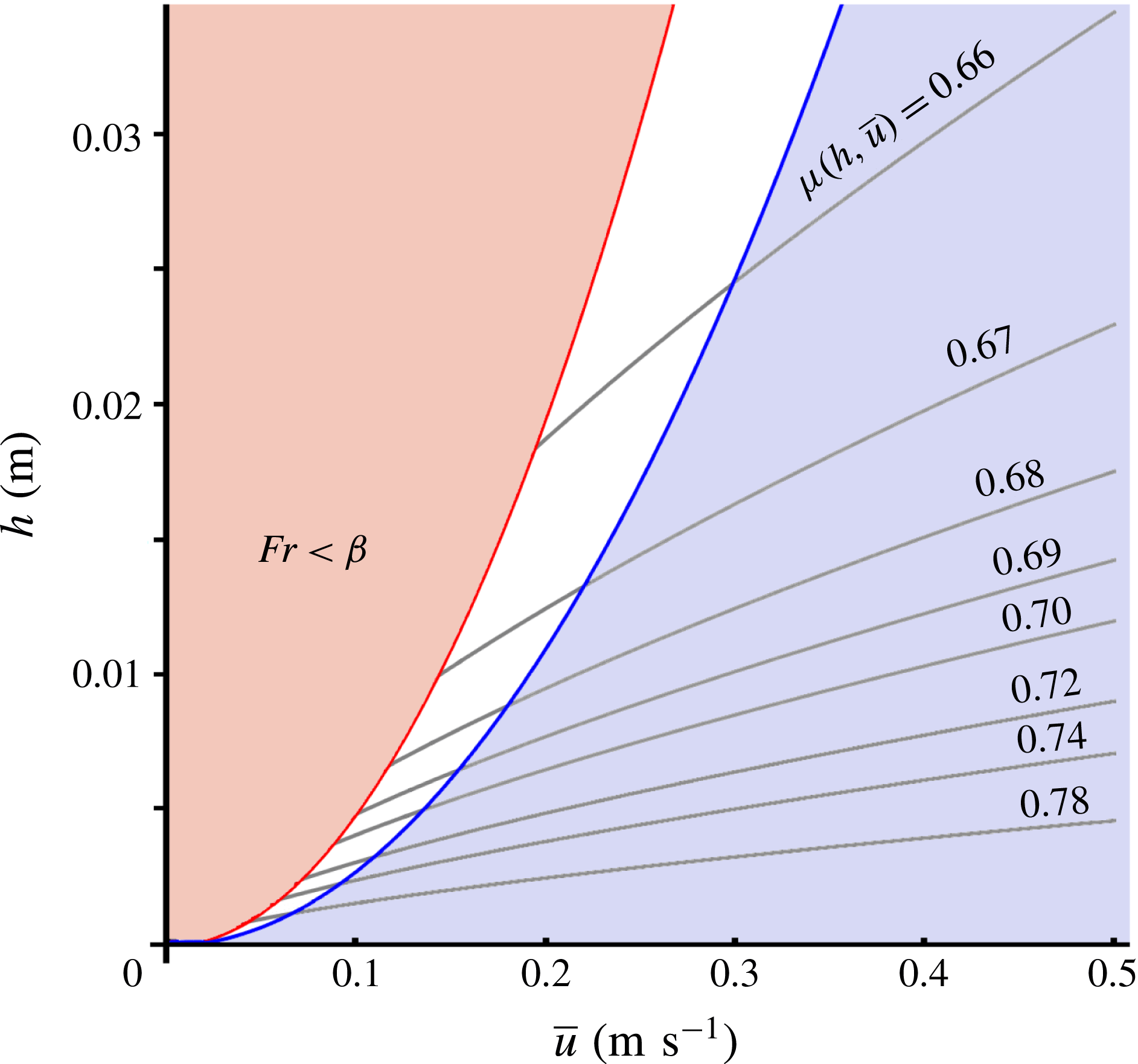
Figure 2 depicts the friction coefficient
 $\unicode[STIX]{x1D707}(h,\bar{u})$
for the above parameter values (and on a chute with tilting angle
 $\unicode[STIX]{x1D701}=33.3^{\circ }$
) as a function of
 $h$
and
 $\bar{u}$
. As one can see,
 $\unicode[STIX]{x1D707}(h,\bar{u})$
is everywhere close to
 $\tan \unicode[STIX]{x1D701}=0.657$
, i.e. the traditional Coulomb dry-friction coefficient for a solid body sliding with constant speed on a chute with inclination angle
 $\unicode[STIX]{x1D701}=33.3^{\circ }$
, yet the departures from this value are of crucial importance for the formation of waves. Monoclinal waves arise in the white region between the two parabolic curves
 $h\propto \bar{u}^{2}$
, which correspond to the lines where the Froude number is equal to
 $\unicode[STIX]{x1D6FD}(=0.50)$
and
 $2/3$
, respectively. Indeed, the physical interpretation of
 $\unicode[STIX]{x1D6FD}$
is that it sets the critical value of the Froude number below which the granular sheet stops flowing.
The friction coefficient
 $\unicode[STIX]{x1D707}(h,\bar{u})$
as a function of the height
 $h$
and depth-averaged velocity
 $\bar{u}$
of the granular sheet, given by (2.4) with the parameter values
 $\unicode[STIX]{x1D6FD}=0.5$
,
 ${\mathcal{L}}=1~\text{mm}$
,
 $\unicode[STIX]{x1D701}_{1}=32.9^{\circ }$
and
 $\unicode[STIX]{x1D701}_{2}=42.0^{\circ }$
. Stable monoclinal waves are possible in the white zone, while roll waves occur in the blue zone to the right; the curve separating these two zones corresponds to
 $Fr=2/3$
. The shaded pink region on the left corresponds to Froude numbers below
 $\unicode[STIX]{x1D6FD}$
(i.e.
 $Fr<0.50$
), where the flow comes to a halt and the given expression for
 $\unicode[STIX]{x1D707}(h,\bar{u})$
does not apply. An extended version of the friction law covering also this region is given in Pouliquen & Forterre (Reference Pouliquen and Forterre2002).

For
 $Fr<\unicode[STIX]{x1D6FD}$
the frictional force outweighs gravity, causing the sheet to be decelerated until it comes to a standstill. This threshold effect has no counterpart in the flow of water but is typical for granular flows. As a matter of fact, the granular sheet does not necessarily have to come to a halt along its entire length, neither does this situation have to be permanent; the Froude number may very well fall below the critical value
 $\unicode[STIX]{x1D6FD}$
only locally, temporarily creating a so-called ‘stopping region’, which at some later stage will be swept into motion again by the new supply of material flowing into this region from above (Edwards & Gray Reference Edwards and Gray2015).
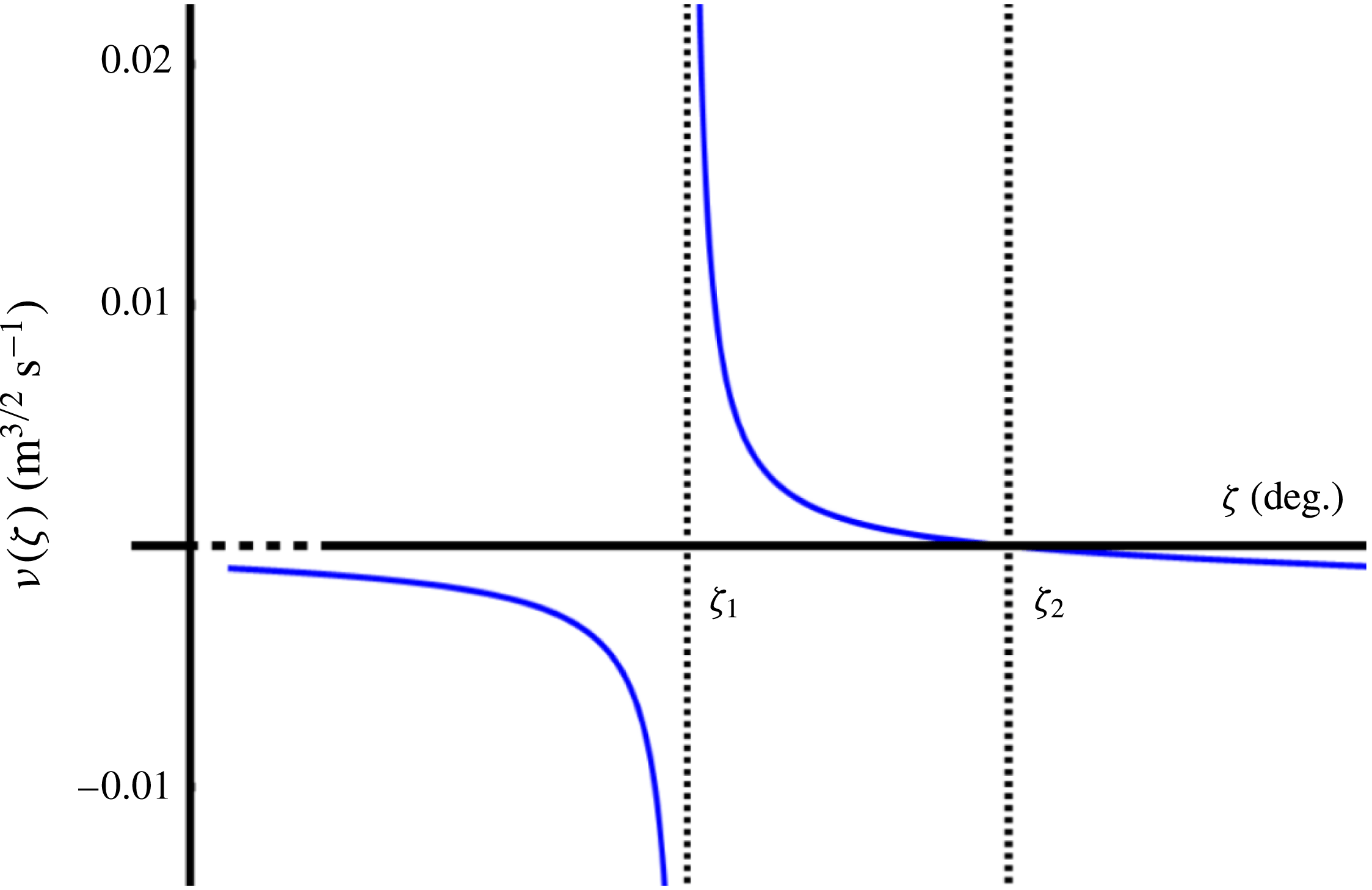
The viscosity coefficient
 $\unicode[STIX]{x1D708}(\unicode[STIX]{x1D701})$
given by (2.5). The coefficient is positive for all inclination angles
 $\unicode[STIX]{x1D701}_{1}<\unicode[STIX]{x1D701}<\unicode[STIX]{x1D701}_{2}$
, i.e. on the whole interval for which steady granular flows are possible. The observation that it is negative outside this interval does not correspond to any intriguing physical effect; it just reflects the fact that the
 $\unicode[STIX]{x1D707}(I)$
-rheology used to derive (2.5) happens to be ill posed here.

One may incorporate the possibility of ‘stopping regions’ in the flow by extending the friction law (2.4) to the regime where
 $Fr<\unicode[STIX]{x1D6FD}$
. The necessary extension has already been given by Pouliquen and Forterre in their original paper on the friction law (2002) but we will not pursue this point in the present study. (An obvious candidate for a granular monoclinal wave with a stopping region is when the lower plateau (height
 $h_{+}$
) happens to be at rest. The coming surge (height
 $h_{-}$
) will then mobilize this layer and the two can be connected in a monoclinal fashion. This will involve an internal erosion wave beneath the upper plateau, separating the parts which are already flowing from those that are still at rest, not unlike the erosion–deposition waves considered by Daerr (Reference Daerr2001) and studied in detail by Edwards & Gray (Reference Edwards and Gray2015) in the context of roll waves with stopping regions. A similar phenomenon occurs when a debris flow surges over a soft deposit layer produced by preceding surges, with the flowing debris eroding and entraining the deposit layer (Takahashi Reference Takahashi2014). We hope to come back to this in a forthcoming publication.) We restrict ourselves to monoclinal waves without stopping regions (as the more direct counterpart of monoclinal waves in water) and this means that the Froude number along the whole profile must exceed
 $\unicode[STIX]{x1D6FD}$
. On the other hand, as mentioned in the introduction, the Froude number should be smaller than
 $2/3$
or else the Kapitza instability will cause the monoclinal wave to break down. Monoclinal waves without stopping regions are possible for
 $\unicode[STIX]{x1D6FD}<Fr<2/3$
.
(iv) The viscous-like diffusive term
 $\unicode[STIX]{x2202}_{x}(\unicode[STIX]{x1D708}h^{3/2}\unicode[STIX]{x2202}_{x}\bar{u})$
, arising from the in-plane stresses in the granular sheet (Gray & Edwards Reference Gray and Edwards2014), with
 $$\begin{eqnarray}\unicode[STIX]{x1D708}=\unicode[STIX]{x1D708}(\unicode[STIX]{x1D701})=\frac{2{\mathcal{L}}\sqrt{g}\sin \unicode[STIX]{x1D701}}{9\unicode[STIX]{x1D6FD}\sqrt{\cos \unicode[STIX]{x1D701}}}\unicode[STIX]{x1D6FE}(\unicode[STIX]{x1D701}),\quad \text{where }\unicode[STIX]{x1D6FE}(\unicode[STIX]{x1D701})=\frac{\tan \unicode[STIX]{x1D701}_{2}-\tan \unicode[STIX]{x1D701}}{\tan \unicode[STIX]{x1D701}-\tan \unicode[STIX]{x1D701}_{1}}.\end{eqnarray}$$
In figure 3 we show how this coefficient
 $\unicode[STIX]{x1D708}(\unicode[STIX]{x1D701})$
depends on the inclination angle
 $\unicode[STIX]{x1D701}$
. In the relevant range
 $\unicode[STIX]{x1D701}_{1}<\unicode[STIX]{x1D701}<\unicode[STIX]{x1D701}_{2}$
, where steady granular flow is possible,
 $\unicode[STIX]{x1D708}(\unicode[STIX]{x1D701})$
is seen to be monotonically decreasing from infinity at
 $\unicode[STIX]{x1D701}=\unicode[STIX]{x1D701}_{1}$
(reflecting the fact that the sheet is stagnant at this limiting angle) to zero at
 $\unicode[STIX]{x1D701}=\unicode[STIX]{x1D701}_{2}$
(heralding the regime of accelerated granular flows). Outside this range, equation (2.5) is seen to give a non-physical negative value for
 $\unicode[STIX]{x1D708}(\unicode[STIX]{x1D701})$
(which would correspond to anti-diffusion rather than diffusion); this is a signature of the fact that the full
 $\unicode[STIX]{x1D707}(I)$
-rheology (GDR-MiDi 2004) used to derive (2.5) is ill posed for high and low inertial numbers, as discussed in Barker et al. (Reference Barker, Schaeffer, Bohorquez and Gray2015).
Gray & Edwards (Reference Gray and Edwards2014) derived this viscous-like term in the momentum balance by depth integrating the
 $\unicode[STIX]{x1D707}(I)$
-rheology and, as a result, were able to obtain continuous and periodic roll wave solutions. Earlier, also Forterre & Pouliquen (Reference Forterre and Pouliquen2003) had already noted that the system (2.2)–(2.3) without such a term is not capable of predicting the correct cutoff frequency for roll waves; to remedy this, following a heuristic approach, Forterre (Reference Forterre2006) enriched the momentum balance with a similar term representing the depth-averaged longitudinal viscous stress.
In the absence of the viscous-like term, a train of roll waves can only be constructed artificially, by piecing together a series of approximately exponential profiles (that would grow indefinitely if they were not cut short) via discontinuous jumps satisfying the Rankine–Hugoniot shock conditions. For roll waves in water, this approach involving discontinuous shocks was the one used in the classic paper on open channel flow by Dressler (Reference Dressler1949). The diffusive term taking into account the in-plane stresses for water (analogous to that for granular matter discussed here), allowing for the spontaneous emergence of a series of roll waves without any discontinuities, was first introduced by Needham & Merkin (Reference Needham and Merkin1984).
Also for monoclinal waves the viscous-like term plays the same role, namely of preventing the profile from developing a discontinuity at its inflection point. This problem does not arise often, since monoclinal waves are usually quite smooth (and the viscous-like term then remains negligibly small along the entire length of the profile), yet it does rear its head when the chute is relatively steep and the amplitude of the wave close to maximal. Under these circumstances the front of the wave can become very sharp and, in the absence of the viscous-like term, it would actually develop a singularity as we will demonstrate in § 4. It is then – and even then only locally around the inflection point – that the viscous-like term grows into a considerable force and saves the situation.
2.2 Steady uniform flow
The most elementary solution admitted by the governing equations of the previous subsection is that of steady uniform flow, i.e. when the sheet is flowing with constant velocity and thickness. In this case, all derivatives with respect to
 $x$
and
 $t$
vanish. So (2.2) is satisfied trivially and the only non-zero terms in (2.3) are those of gravity and friction (the first and the third term on the right-hand side), meaning that these must precisely balance each other:
 $\tan \unicode[STIX]{x1D701}=\unicode[STIX]{x1D707}(h,\bar{u})$
. Denoting the uniform thickness by
 $h_{0}$
, the corresponding depth-averaged velocity is then found to be, through (2.4):
 $$\begin{eqnarray}\bar{u}_{0}=\frac{\unicode[STIX]{x1D6FD}\sqrt{g\cos \unicode[STIX]{x1D701}}}{{\mathcal{L}}\unicode[STIX]{x1D6FE}(\unicode[STIX]{x1D701})}h_{0}^{3/2}.\end{eqnarray}$$
The corresponding Froude number measured in the laboratory frame is:
 $$\begin{eqnarray}Fr=\frac{\bar{u}_{0}}{\sqrt{gh_{0}\cos \unicode[STIX]{x1D701}}}=\frac{\unicode[STIX]{x1D6FD}}{{\mathcal{L}}\unicode[STIX]{x1D6FE}(\unicode[STIX]{x1D701})}h_{0},\end{eqnarray}$$
which is a linearly increasing function of the sheet thickness. This means that for the monoclinal wave, which consists of two uniform sheets linked through a shock structure, the incoming sheet (with height
 $h_{-}$
and averaged velocity
 $\bar{u}_{-}$
) has a higher Froude number than the outgoing sheet (with
 $h_{+}$
and
 $\bar{u}_{+}$
). So, for a granular monoclinal wave without stopping regions, the following inequality must hold:
 $$\begin{eqnarray}\unicode[STIX]{x1D6FD}<Fr(h_{+},\bar{u}_{+})<Fr(h_{-},\bar{u}_{-})<{\textstyle \frac{2}{3}}.\end{eqnarray}$$
2.3 A phase diagram for finding granular monoclinal waves
As a preview to the sections that follow, we note that the above constitutive relations (and in particular the friction law) determine the zone in the
 $(\unicode[STIX]{x1D701},h)$
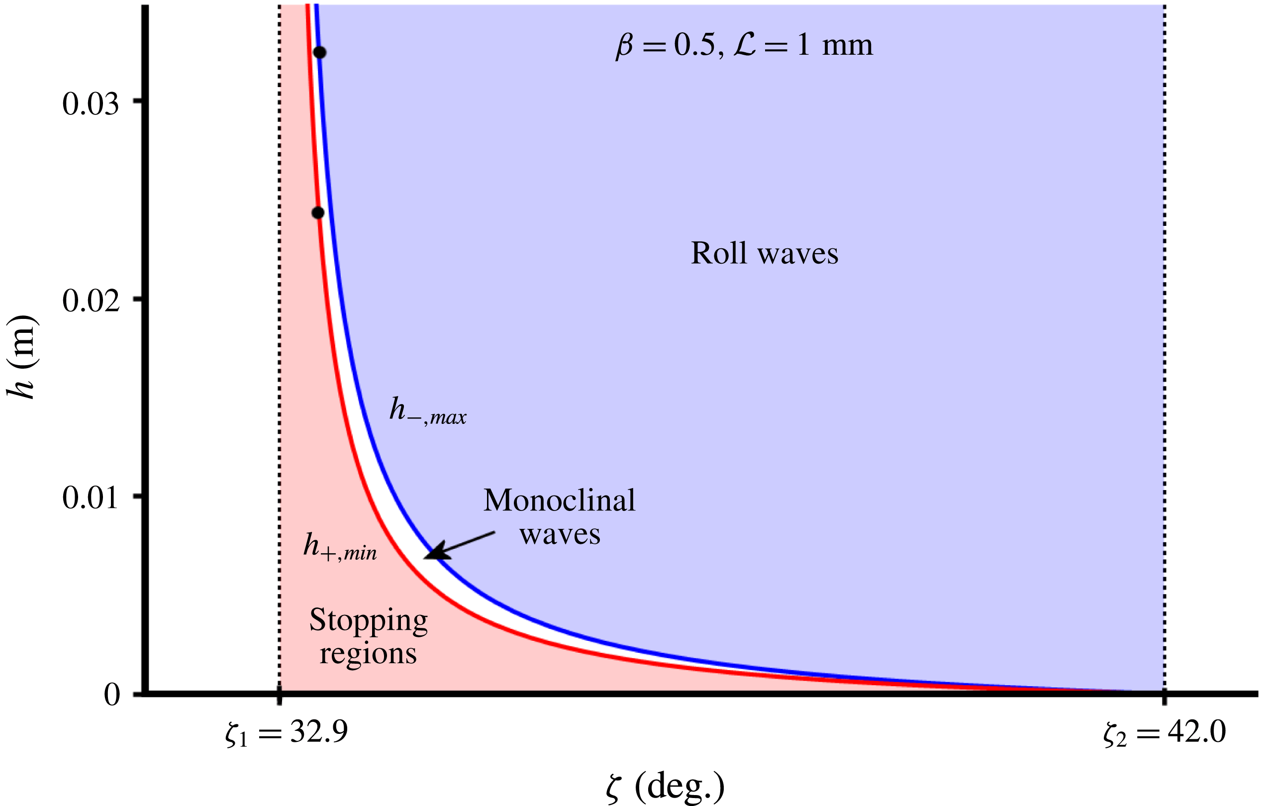
plane where stable monoclinal waves may be expected to arise. As mentioned above, we restrict ourselves to monoclinal waves without static regions. In figure 4 we depict this zone of stability (the white zone) for the typical parameter values
 $\unicode[STIX]{x1D6FD}=0.5$
,
 ${\mathcal{L}}=1~\text{mm}$
,
 $\unicode[STIX]{x1D701}_{1}=32.9^{\circ }$
and
 $\unicode[STIX]{x1D701}_{2}=42.0^{\circ }$
which will also be used in the rest of the text.
Phase diagram depicting the region in the
 $(\unicode[STIX]{x1D701},h)$
plane where stable granular monoclinal waves without stopping regions occur. Here
 $\unicode[STIX]{x1D701}$
is the inclination angle of the chute – which must lie between
 $\unicode[STIX]{x1D701}_{1}$
and
 $\unicode[STIX]{x1D701}_{2}$
– and
 $h$
is the thickness of the granular sheet, which for a monoclinal wave runs from the high plateau value
 $h_{-}$
to the lower plateau value
 $h_{+}$
. Three regions can be distinguished: (i) if the thickness
 $h_{+}$
of the lower plateau falls below the curve
 $h_{+,min}$
, corresponding to
 $Fr<\unicode[STIX]{x1D6FD}$
, the low plateau is decelerated and develops stopping regions; (ii) for system parameters within the blank region (
 $\unicode[STIX]{x1D6FD}<Fr<2/3$
) we find stable monoclinal waves with both plateaus flowing; (iii) the region above the curve
 $h_{-,max}$
corresponds to
 $Fr>2/3$
, where the Kapitza instability renders monoclinal waves unstable and induces the formation of roll waves. The curves
 $h_{+,min}(\unicode[STIX]{x1D701})$
and
 $h_{-,max}(\unicode[STIX]{x1D701})$
represent the minimum thickness of the low plateau and the maximum thickness of the high one, respectively. The two black dots on these curves delimit the zone of stable monoclinal waves for
 $\unicode[STIX]{x1D701}=33.3^{\circ }$
. The present figure is made for the typical parameter values
 $\unicode[STIX]{x1D6FD}=0.5$
,
 ${\mathcal{L}}=1~\text{mm}$
,
 $\unicode[STIX]{x1D701}_{1}=32.9^{\circ }$
and
 $\unicode[STIX]{x1D701}_{2}=42.0^{\circ }$
, which are used throughout the text.

The left and right boundaries (
 $\unicode[STIX]{x1D701}_{1}$
and
 $\unicode[STIX]{x1D701}_{2}$
respectively) speak for themselves. The curved upper and lower boundaries of the white zone are dictated by the interval of suitable Froude numbers,
 $\unicode[STIX]{x1D6FD}<Fr<2/3$
, and more specifically by the inequality (2.8).
A uniform granular sheet will come to a halt when its thickness
 $h$
and related velocity
 $\bar{u}$
given by (2.6) are such that the Froude number falls below the threshold value
 $\unicode[STIX]{x1D6FD}$
. It may also lie still in the first place, with
 $Fr=0$
. Since in the present paper we are interested in monoclinal waves for which both plateaus are moving, this gives a minimum value for the thickness of the low plateau, cf. (2.7):
 $$\begin{eqnarray}h_{+,min}(\unicode[STIX]{x1D701})={\mathcal{L}}\unicode[STIX]{x1D6FE}(\unicode[STIX]{x1D701})={\mathcal{L}}\frac{\tan \unicode[STIX]{x1D701}_{2}-\tan \unicode[STIX]{x1D701}}{\tan \unicode[STIX]{x1D701}-\tan \unicode[STIX]{x1D701}_{1}}.\end{eqnarray}$$
On the other hand, when the thickness of the granular sheet (and the related velocity) become so large that
 $Fr$
exceeds the critical value
 $2/3$
, the uniform sheet will be destabilized by the Kapitza instability and break into a series of granular roll waves. This gives an upper value for the thickness of the high plateau of the monoclinal wave, again invoking (2.7):
 $$\begin{eqnarray}h_{-,max}(\unicode[STIX]{x1D701})=\frac{2{\mathcal{L}}}{3\unicode[STIX]{x1D6FD}}\unicode[STIX]{x1D6FE}(\unicode[STIX]{x1D701})=\frac{2{\mathcal{L}}}{3\unicode[STIX]{x1D6FD}}\frac{\tan \unicode[STIX]{x1D701}_{2}-\tan \unicode[STIX]{x1D701}}{\tan \unicode[STIX]{x1D701}-\tan \unicode[STIX]{x1D701}_{1}}.\end{eqnarray}$$
It is only in the intermediate zone between
 $h_{+,min}(\unicode[STIX]{x1D701})$
and
 $h_{-,max}(\unicode[STIX]{x1D701})$
that one may expect to find stable monoclinal waves with both plateaus moving. For inclination angles
 $\unicode[STIX]{x1D701}$
close to
 $\unicode[STIX]{x1D701}_{1}$
this region is reasonably wide, meaning that the plateau values
 $h_{-}$
and
 $h_{+}$
may be relatively far apart, making the monoclinal waves easily detectable. To facilitate things further, it is advisable to use particles for which
 $\unicode[STIX]{x1D6FD}$
is smaller than our standard value of
 $0.5$
, e.g. smooth spherical glass beads (Pouliquen & Forterre Reference Pouliquen and Forterre2002); the lower boundary
 $h_{+,min}$
of the stability zone will then go down (or equivalently, the stopping region shrinks) and hence the difference between the plateau values can be larger. We will explore this in more detail in § 6, where we describe the optimal conditions for detecting granular monoclinal waves in experiment.
For increasing inclination angles, the region narrows swiftly and for
 $\unicode[STIX]{x1D701}\rightarrow \unicode[STIX]{x1D701}_{2}$
the plateau values lie necessarily so close to each other that experimental detection of the associated monoclinal waves will be extremely difficult, or even impossible when the difference between
 $h_{+,min}(\unicode[STIX]{x1D701})$
and
 $h_{-,max}(\unicode[STIX]{x1D701})$
becomes less than a particle diameter.
Formation of a monoclinal wave on a chute with inclination angle
 $\unicode[STIX]{x1D701}=33.3^{\circ }$
. We start from an initial profile consisting of two plateaus of uniform flow, connected in a smooth but arbitrary way, with the Froude number of the high plateau
 $Fr(h_{-},\bar{u}_{-})=0.595$
lying well within the appropriate range
 $\unicode[STIX]{x1D6FD}(=0.5)<Fr<2/3$
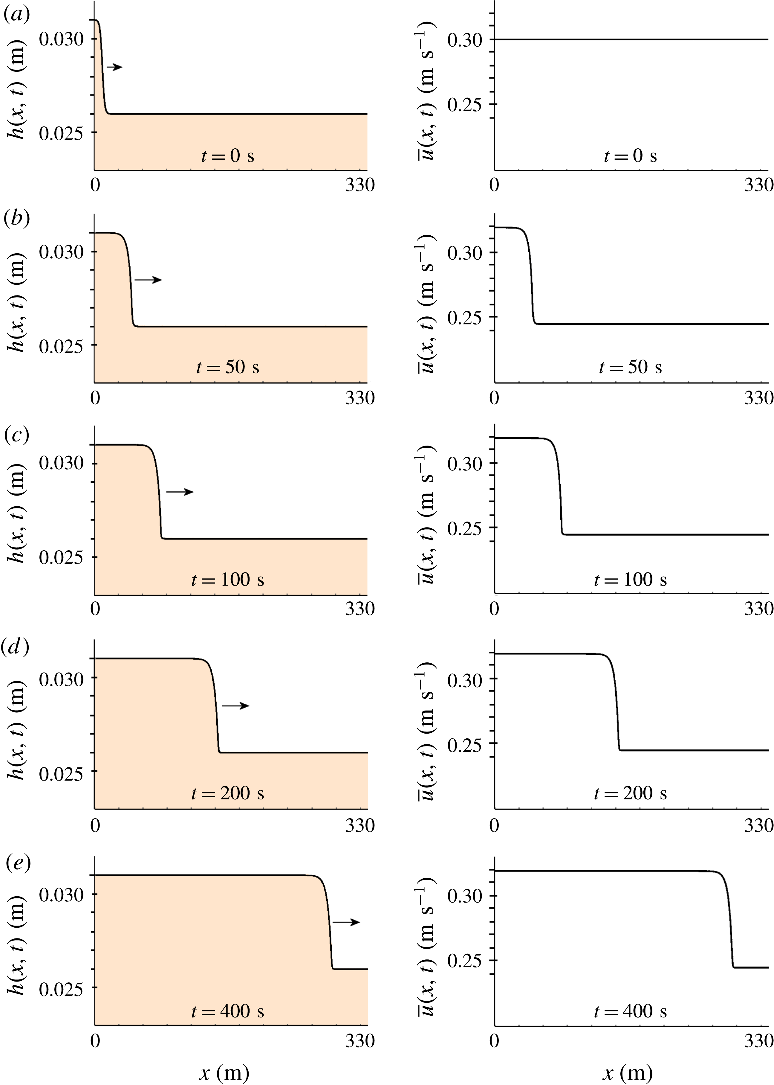
. Numerically solving (2.2)–(2.3), we find that the profile gradually ripens to a fixed shape, consisting of a long exponential descent, stretching out over tens of metres, followed by a relatively sharp bend where the wave front joins onto the lower plateau. In the last snapshot at
 $t=400~\text{s}$
, the wave propagates downstream at
 $0.69~\text{m}~\text{s}^{-1}$
, which is very close to the final wave speed
 $c=0.70~\text{m}~\text{s}^{-1}$
given by (2.11).

On the basis of the above phase diagram we now perform a numerical experiment. Using the same parameter values as in figure 4 (
 $\unicode[STIX]{x1D6FD}=0.5$
,
 ${\mathcal{L}}=1~\text{mm}$
,
 $\unicode[STIX]{x1D701}_{1}=32.9^{\circ }$
and
 $\unicode[STIX]{x1D701}_{2}=42.0^{\circ }$
) and choosing the inclination angle
 $\unicode[STIX]{x1D701}=33.3^{\circ }$
, we start from the initial condition depicted in the upper row of figure 5: a height profile smoothly connecting a high plateau at 31.0 mm with a lower one at 26.0 mm (both within the white zone of the phase diagram for the given inclination angle, see figure 4) and a constant velocity of
 $0.30~\text{m}~\text{s}^{-1}$
along the entire length of the sheet. That is, the Froude number of the incoming sheet is
 $Fr(h_{-},\bar{u}_{-})=0.595$
, well within the prescribed range of
 $\unicode[STIX]{x1D6FD}<Fr<2/3$
. The chosen initial velocity
 $\bar{u}(x,0)$
is such that the Froude number for the outgoing sheet is
 $0.65$
, which momentarily violates the condition
 $Fr(h_{+},\bar{u}_{+})<Fr(h_{-},\bar{u}_{-})$
. This is done intentionally, to show that the system is capable of repairing this inverted state of affairs.
For the numerical integration of the two coupled partial differential equations (2.2)–(2.3), we use the ‘method of lines’ (Schiesser Reference Schiesser1991; Hamdi, Schiesser & Griffiths Reference Hamdi, Schiesser and Griffiths2007). This method transforms the two partial differential equations (PDEs) into a system of ordinary differential equations (ODEs), by discretizing the spatial variable
 $x$
to a uniform grid (
 $0\leqslant x_{i}\leqslant x_{max}$
in steps of
 $\unicode[STIX]{x0394}x$
) and using a central-difference scheme to approximate the spatial derivatives, leaving
 $t$
as the only continuous independent variable. To produce figure 5 we chose
 $x_{max}=340$
with a grid spacing
 $\unicode[STIX]{x0394}x=0.02$
. (The accuracy of the results was checked by repeating the procedure for various values of the grid spacing. In particular, we have also used
 $\unicode[STIX]{x0394}x=0.03$
and
 $\unicode[STIX]{x0394}x=0.01$
and found that the resulting monoclinal profiles were indistinguishable from each other on the scale of figure 5.) The resulting system of ODEs then consists of
 $x_{max}/\unicode[STIX]{x0394}x+1=17\,001$
equations per PDE, leading to a total of
 $34\,002$
coupled ODEs.
This system of ODEs (with the initial conditions being the values of
 $h(x,0)$
and
 $\bar{u}(x,0)$
shown in the top row of figure 5, at the grid points
 $x=x_{i}$
,
 $i=1\cdots 17001$
) was subsequently solved with the so-called LSODA algorithm, which employs both stiff and non-stiff methods. This algorithm uses the Adams method for non-stiff regions and, whenever stiffness is detected, switches to a variable-step, variable-order backwards difference formula. The numerical evaluation of the results depicted in figure 5 required 60 GB Ram.
The fate of a monoclinal-type profile with Froude number of the upper plateau
 $Fr=0.80$
, i.e. above the threshold value
 $Fr=2/3$
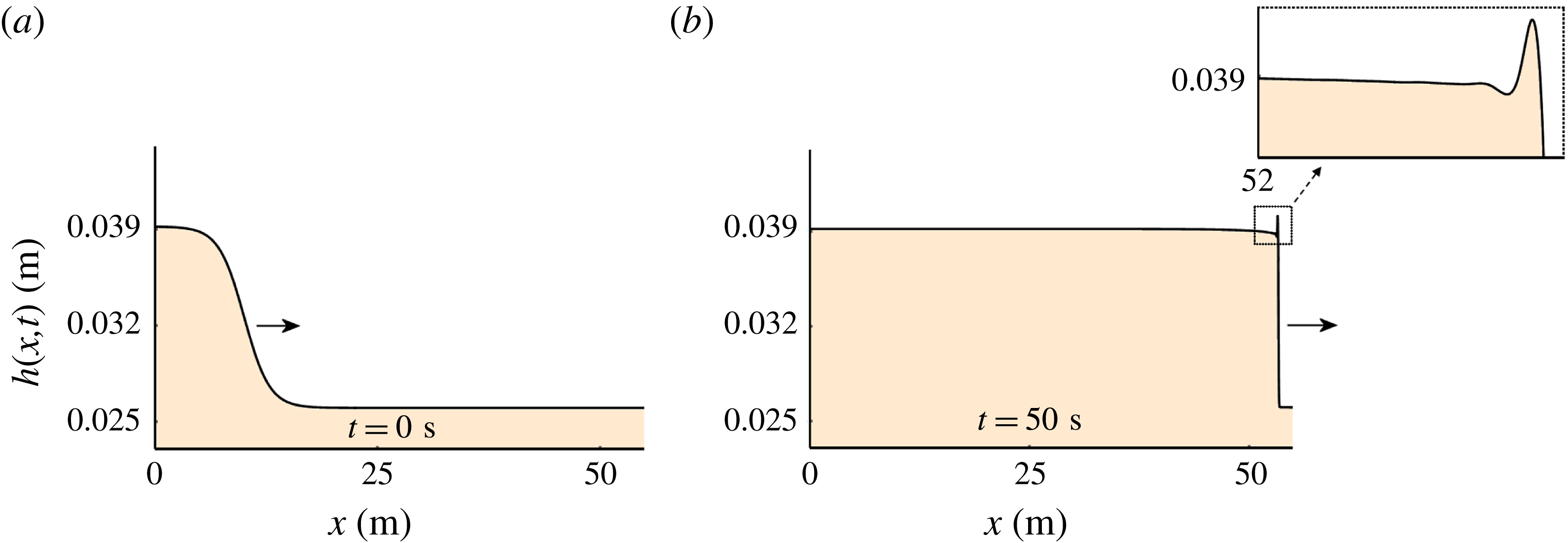
. Starting from a similar initial state as in figure 5, numerical integration of (2.2)–(2.3) reveals that now a hump is formed at the steepening front, disrupting the monotonic descent of the profile. This hump is due to the Kapitza instability.

The thus computed profiles, presented in the consecutive snapshots of figure 5, show that the initial condition gradually develops into a proper monoclinal wave. The Froude numbers in the final snapshot, at
 $t=400~\text{s}$
, are
 $Fr(h_{-},\bar{u}_{-})=0.63$
and
 $Fr(h_{+},\bar{u}_{+})=0.53$
. To the best of our knowledge, this is the first granular monoclinal wave without stopping regions reported in the literature.
While the shape of the wave assumes its final form, its speed gradually converges to a constant value given by the well-known formula for the speed of shock waves (Whitham Reference Whitham1974):
 $$\begin{eqnarray}c=\frac{h_{-}\bar{u}_{-}-h_{+}\bar{u}_{+}}{h_{-}-h_{+}}.\end{eqnarray}$$
The above relation expresses the fact that, for an observer in the co-moving frame, the flux of material entering the shock structure must be equal to the flux leaving the shock, i.e.
 $h_{+}(\bar{u}_{+}-c)=h_{-}(\bar{u}_{-}-c)$
. This conservation principle leads directly to (2.11). Note that the velocities of the two plateaus are
 $\bar{u}_{-}=0.319~\text{m}~\text{s}^{-1}$
and
 $\bar{u}_{+}=0.245~\text{m}~\text{s}^{-1}$
, and with
 $h_{-}=0.031~\text{m}$
and
 $h_{+}=0.026~\text{m}$
this gives
 $c=0.70~\text{m}~\text{s}^{-1}$
, so that
 $c>\bar{u}_{-}>\bar{u}_{+}$
just as for monoclinal waves in water (cf. figure 1).
The shape of the wave in its ripened form is characterized by a long exponential descent, stretched out over tens of metres (three to four orders of magnitude larger than the amplitude
 $\unicode[STIX]{x0394}h=h_{-}-h_{+}=5~\text{mm}$
), followed by a relatively sharp bend where the wave front meets the lower region of uniform flow. In the next sections we will study these properties in detail.
Here, in order to demonstrate that monoclinal waves only appear when the Froude number is in the appropriate range, we show in figure 6 what happens to an initial monoclinal-like profile with
 $Fr(h_{-},\bar{u}_{-})=0.80$
, i.e. above the threshold value of
 $Fr=2/3$
. Very soon the Kapitza instability manifests itself: a protrusion is formed on the upper flank of the wave, destroying the monoclinal nature of the profile. In due time, this protrusion will ripen into a roll wave.
3 Travelling wave analysis
3.1 The ODE governing the fully ripened monoclinal wave
Since the monoclinal wave is a waveform propagating with a constant wave speed
 $c$
, the natural way to extract it from (2.2) and (2.3) is to introduce the travelling wave ansatz, with the new variable
 $\unicode[STIX]{x1D709}=x-ct$
. That is, we concentrate on solutions of the type:
 $$\begin{eqnarray}h(x,t)=h(x-ct)=h(\unicode[STIX]{x1D709})\quad \text{and}\quad \bar{u}(x,t)=\bar{u}(x-ct)=\bar{u}(\unicode[STIX]{x1D709}).\end{eqnarray}$$
Substituting the ansatz (3.1) into the mass balance (2.2) and denoting the differentiation with respect to
 $\unicode[STIX]{x1D709}$
with a prime, we obtain
 $-ch^{\prime }+(h\bar{u})^{\prime }=0$
, which can readily be integrated to give:
 $$\begin{eqnarray}-ch+h\bar{u}=-K.\end{eqnarray}$$
Here
 $K=|h(\bar{u}-c)|$
is a positive constant representing the volumetric flux per unit width of the chute as measured in the co-moving frame (travelling at speed
 $c$
). The fact that this flux must be constant to an observer in the co-moving frame was already noted in the context of (2.11). Since the wave speed
 $c>\bar{u}_{-}>\bar{u}_{+}$
, the observer in the co-moving frame sees the particles pass by in the upstream direction, in such a way that the particles in the thin sheet move with a relative velocity
 $\bar{u}_{+}-c$
that is larger (i.e. more negative) than the relative velocity
 $\bar{u}_{-}-c$
in the thick sheet. More specifically,
 $\bar{u}_{+}-c=(h_{-}/h_{+})(\bar{u}_{-}-c)$
, in accordance with the principle of continuity.
As for the momentum balance equation (2.3), we first note that the left-hand side, with the aid of the continuity equation (2.2), can be cast in the form
 $h(\unicode[STIX]{x2202}_{t}\bar{u}+\bar{u}\unicode[STIX]{x2202}_{x}\bar{u})$
. Then, upon substituting the travelling wave ansatz (3.1) and dividing throughout by
 $h$
, the momentum balance becomes:
 $$\begin{eqnarray}-c\bar{u}^{\prime }+\bar{u}\bar{u}^{\prime }=g\sin \unicode[STIX]{x1D701}-g\cos \unicode[STIX]{x1D701}h^{\prime }-\unicode[STIX]{x1D707}(h,\bar{u})g\cos \unicode[STIX]{x1D701}+\unicode[STIX]{x1D708}({\textstyle \frac{3}{2}}h^{-1/2}h^{\prime }\bar{u}^{\prime }+h^{1/2}\bar{u}^{\prime \prime }).\end{eqnarray}$$
Now, with the use of (3.2) we can eliminate
 $\bar{u}(\unicode[STIX]{x1D709})$
and its derivatives from this equation. First we use (3.2) to write
 $\bar{u}=c-Kh^{-1}$
, and hence
 $\bar{u}^{\prime }=Kh^{-2}h^{\prime }$
and
 $\bar{u}^{\prime \prime }=-2Kh^{-3}(h^{\prime })^{2}+Kh^{-2}h^{\prime \prime }$
, and then we insert these three expressions into (3.3) to obtain a second-order ordinary differential equation for
 $h(\unicode[STIX]{x1D709})$
alone:
 $$\begin{eqnarray}\frac{\unicode[STIX]{x1D708}K}{h^{3/2}}h^{\prime \prime }-\frac{\unicode[STIX]{x1D708}K}{2h^{5/2}}(h^{\prime })^{2}+\left(\frac{K^{2}}{h^{3}}-g\cos \unicode[STIX]{x1D701}\right)h^{\prime }+g\sin \unicode[STIX]{x1D701}-\unicode[STIX]{x1D707}(h)g\cos \unicode[STIX]{x1D701}=0.\end{eqnarray}$$
This is the equation that governs the shape of the granular monoclinal wave in its fully ripened form. Note that also the friction coefficient
 $\unicode[STIX]{x1D707}(h,\bar{u})$
, after the substitution
 $\bar{u}=c-Kh^{-1}$
from (3.2), is a function of
 $h$
alone. To be specific, the form
 $\unicode[STIX]{x1D707}(h)$
in which it appears in (3.4) is:
 $$\begin{eqnarray}\unicode[STIX]{x1D707}(h)=\tan \unicode[STIX]{x1D701}_{1}+\frac{\tan \unicode[STIX]{x1D701}_{2}-\tan \unicode[STIX]{x1D701}_{1}}{1+\unicode[STIX]{x1D6FD}{\mathcal{L}}^{-1}\sqrt{g\cos \unicode[STIX]{x1D701}}h^{5/2}/(ch-K)}.\end{eqnarray}$$
Equation (3.4) can be solved numerically using the appropriate boundary conditions. We need one condition for the first derivative
 $\text{d}h/\text{d}\unicode[STIX]{x1D709}$
(at some point
 $\unicode[STIX]{x1D709}=\unicode[STIX]{x1D709}_{0}$
along the profile) and one for
 $h(\unicode[STIX]{x1D709})$
itself. Here an interesting problem arises: we wish to find a waveform that satisfies the conditions
 $h(\unicode[STIX]{x1D709})=h_{-}$
for
 $\unicode[STIX]{x1D709}\rightarrow -\infty$
and
 $h(\unicode[STIX]{x1D709})=h_{+}$
for
 $\unicode[STIX]{x1D709}\rightarrow \infty$
, while also attaining a zero slope at
 $\unicode[STIX]{x1D709}\rightarrow \pm \infty$
, which are more conditions than one usually imposes on a second-order ODE.
One might at first be tempted to use a shooting method at the physical boundaries of the system to solve (3.4). Unfortunately, this turns out to work poorly, since typically such a method tries to connect the height
 $h_{-}$
smoothly to
 $h_{+}$
by ‘shooting’ for the appropriate slope with which the profile departs from
 $h_{-}$
. This slope, however, is extremely close to zero (and becomes exactly zero for
 $\unicode[STIX]{x1D709}\rightarrow \pm \infty$
) and thus the shooting algorithm is forced to explore tiny slope values close to the machine accuracy. This results in a very unstable and inaccurate calculation of the profile.
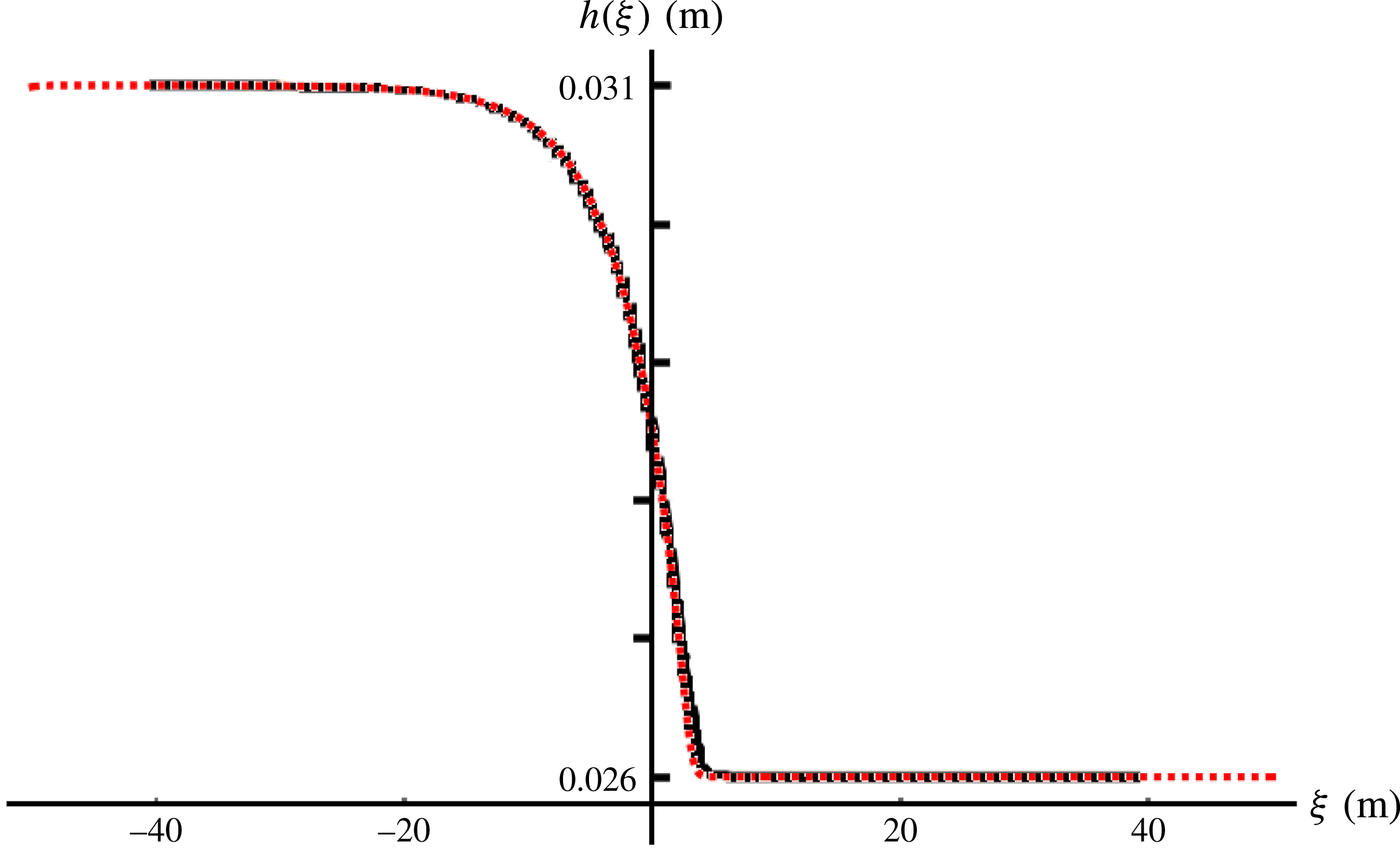
The monoclinal wave solution
 $h_{full}(\unicode[STIX]{x1D709})$
of the second-order ODE (3.4), red dashed line, together with the profile
 $h(x,t)$
at
 $t=400~\text{s}$
of figure 5(e), solid black line. The two profiles are seen to coincide to a large extent, meaning that the latter (solid line) is well on its way of converging to the exact monoclinal waveform represented by the red dashed line. In fact, the only part where the convergence is not yet perfect is around the relatively sharp bend where the upper flank of the profile meets the lower plateau of height
 $h_{+}$
.

To avoid the difficulty caused by the null slope at the plateaus, we decided to choose a reference point somewhere in the intermediate region. It turns out that we get good results by prescribing the values for
 $h(\unicode[STIX]{x1D709}_{0})$
and
 $h^{\prime }(\unicode[STIX]{x1D709}_{0})$
at a point
 $\unicode[STIX]{x1D709}_{0}$
where the wave front is just about to connect to the lower plateau. This particular choice of
 $\unicode[STIX]{x1D709}_{0}$
is inspired by the fact that the ODE (3.4) has the property of yielding a well-behaved, converging solution for
 $\unicode[STIX]{x1D709}<\unicode[STIX]{x1D709}_{0}$
whereas it tends to diverge violently for
 $\unicode[STIX]{x1D709}>\unicode[STIX]{x1D709}_{0}$
. In essence, we shoot from a point
 $\unicode[STIX]{x1D709}=\unicode[STIX]{x1D709}_{0}$
close to the low plateau value
 $h_{+}$
, but not too close, such that the derivative
 $h^{\prime }(\unicode[STIX]{x1D709}_{0})$
has an appreciable non-zero value, and aim for the high plateau.
The corresponding solution
 $h_{full}(\unicode[STIX]{x1D709})$
of (3.4), shown in figure 7, is seen to agree very well with the wave depicted in figure 5(e), which was obtained by numerical evaluation (for 400 seconds) of the two governing balance equations (2.2)–(2.3).
The slight difference between the solid and dashed lines can be attributed to the fact that the numerical solution of the balance equations (2.2)–(2.3) has not yet fully ripened to its final shape yet, which is no other than
 $h_{full}(\unicode[STIX]{x1D709})$
. The profile of figure 5(e) is well on its way after
 $t=400~\text{s}$
, which is the limit of our computational power, yet to make it really indistinguishable from the solution of (3.4) (on the scale of figure 7) more time would be needed. Another and even more direct way of showing that the solution of (3.4) (red dashed line) is the true, fully ripened monoclinal profile, is to use this solution (and the corresponding velocity profile) as initial conditions for the system of PDEs (2.2)–(2.3). We did so and witnessed that the height and velocity profiles remained totally unaltered, proving the point.
In the
 $(h,h^{\prime })$
plane, the monoclinal wave takes the form of a heteroclinic connection between the fixed points
 $(h_{-},0)$
and
 $(h_{+},0)$
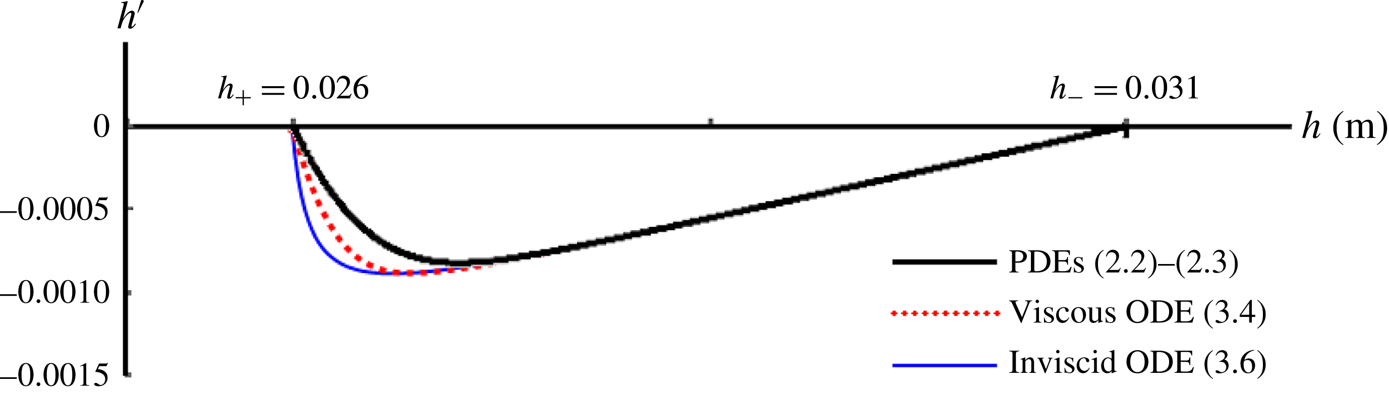
, corresponding to the two flat plateaus. Here we compare: (i) the not yet fully ripened profile
 $h(x,t)$
at
 $t=400~\text{s}$
of figure 5(e), solid black line, obtained from the governing partial differential equations, i.e. PDEs (2.2)–(2.3); (ii) the monoclinal wave solution
 $h_{full}(\unicode[STIX]{x1D709})$
of the viscous second-order ODE (3.4), red dashed line; and (iii) its inviscid counterpart
 $h_{inv}(\unicode[STIX]{x1D709})$
obtained from the first-order ODE (3.6), thin blue line. The exact monoclinal waveform is represented by the red dashed line (middle curve). The three lines agree exceedingly well along their straight sections, corresponding to the long exponentially descending upper flank of the monoclinal wave. The lines depart from each other only in a small region between the inflection point (where the slope
 $h^{\prime }$
goes through its minimum) and the point
 $(h_{+},0)$
, where the wave connects to the lower plateau. See also figure 7 for the profiles (i) and (ii), and figure 9 for the profiles (ii) and (iii).

To highlight the incomplete convergence of the solid profile presented in figure 7, and to make it more conspicuous than in the usual visualization of
 $h(\unicode[STIX]{x1D709})$
versus
 $\unicode[STIX]{x1D709}$
, we also plot the slope
 $h^{\prime }(\unicode[STIX]{x1D709})$
versus
 $h(\unicode[STIX]{x1D709})$
for both curves. This is done in figure 8.
Let us concentrate on the two curves corresponding to the numerical solution of the PDEs (solid black line,
 $\unicode[STIX]{x2202}h(x,t)/\unicode[STIX]{x2202}x$
of the snapshot at
 $t=400~\text{s}$
in figures 5 and 7) and that of the second-order ODE (dashed red line,
 $\text{d}h_{full}(\unicode[STIX]{x1D709})/\text{d}\unicode[STIX]{x1D709}$
, cf. figure 7): both lines are seen to exhibit a long straight segment emanating from
 $(h_{-},0)$
, corresponding to the long exponential descending part of the monoclinal wave. This straight segment ends where the slope
 $h^{\prime }$
goes through its minimum, i.e. at the inflection point of the monoclinal profile. After that, the slope steeply rises again, until it becomes zero where the wave profile joins onto the low plateau at
 $(h_{+},0)$
. Note that the quantities
 $h^{\prime }$
and
 $h$
in this plot have been deliberately chosen such as to bring out the small differences between the profiles (around the inflection point) as clearly as possible. As mentioned before, the black solid curve is on its way to converge to the red dashed curve; that is, if we had taken a snapshot at some later stage
 $(t>400~\text{s})$
we would have found another black curve lying closer to the dashed one.
As an aside, we note that figure 8 demonstrates that the monoclinal wave corresponds to a heteroclinic connection in the
 $(h,h^{\prime })$
plane between the fixed points
 $(h_{-},0)$
and
 $(h_{+},0)$
. (In dynamical systems theory, a heteroclinic connection in the phase plane
 $(h,h^{\prime })$
is a trajectory connecting two different fixed points, such as
 $(h_{-},0)$
and
 $(h_{+},0)$
. It may be contrasted with a homoclinic connection, which is a trajectory that starts and ends at the same fixed point.) The name ‘monoclinal wave’ (referring to the fact that the profile
 $h(\unicode[STIX]{x1D709})$
consists of a single flank descending from height
 $h_{-}$
to
 $h_{+}$
) may cause some confusion in this respect. For the sake of tradition we stick to this name, but not without a word of caution to the reader.
Here we also note that the viscous-like term has only a minor effect on the form of the monoclinal wave. By taking the inviscid limit
 $\unicode[STIX]{x1D708}\rightarrow 0$
of (3.4), one obtains a first-order ordinary differential equation,
 $$\begin{eqnarray}\left(\frac{K^{2}}{h^{3}}-g\cos \unicode[STIX]{x1D701}\right)h^{\prime }+g\sin \unicode[STIX]{x1D701}-\unicode[STIX]{x1D707}(h)g\cos \unicode[STIX]{x1D701}=0,\end{eqnarray}$$
which must be accompanied by one boundary condition; we choose
 $h(0)=(h_{-}+h_{+})/2$
, exactly midway between the two plateau heights. The resulting profiles are in most cases (see however § 4) virtually indistinguishable from the one with viscosity. Only the bend where the profile connects to the low-level plateau is slightly sharper, just as one would expect when one discards viscosity. The small difference is illustrated in figure 8, where the thin blue line (the lowest of the three curves) represents the slope
 $\text{d}h/\text{d}\unicode[STIX]{x1D709}$
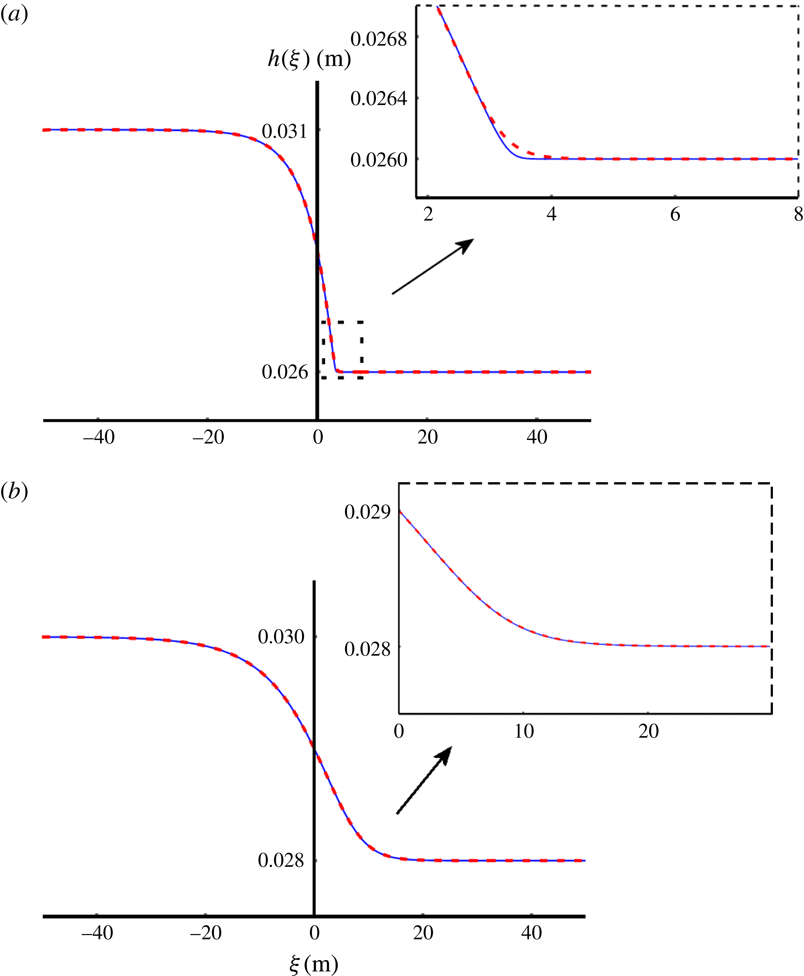
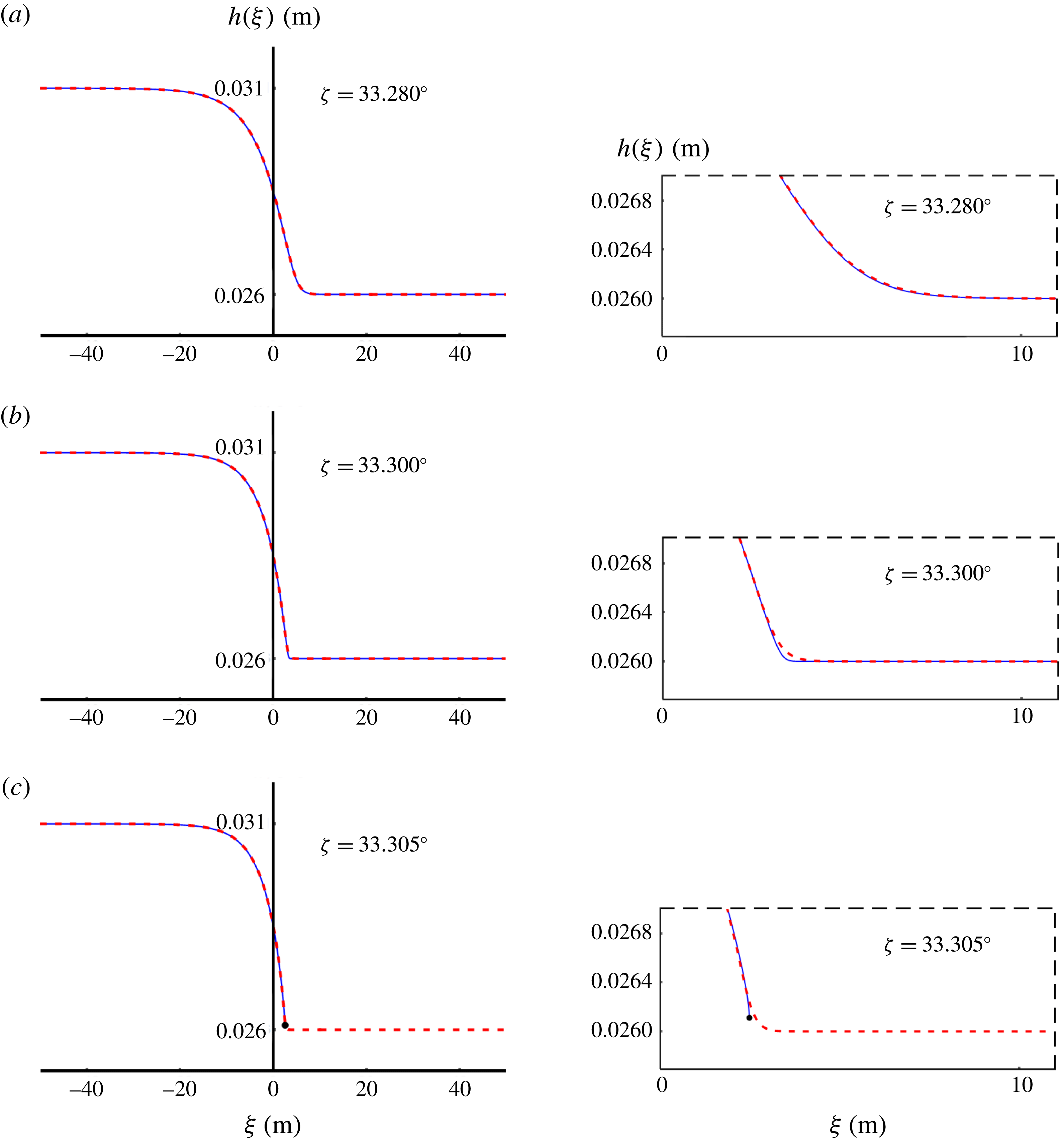
of the monoclinal wave in the absence of viscosity. The difference is also presented in figure 9(a), where we put the two solutions
 $h_{full}(\unicode[STIX]{x1D709})$
(of the second-order ODE (3.4)) and
 $h_{inv}(\unicode[STIX]{x1D709})$
(of the inviscid first-order ODE (3.6)) side by side. Just as in the other figures, the former is represented by a red dashed line and the latter by a solid blue line. We notice that the two profiles are almost indistinguishable, except when one zooms in on the narrow region where they join onto the lower plateau: the exact monoclinal wave (with viscosity) does this somewhat more smoothly than its inviscid counterpart, and even this difference becomes utterly negligible when the amplitude
 $\unicode[STIX]{x0394}h=h_{-}-h_{+}$
is small (see figure 9
b). Consequently, it is fully justified to have a closer look at the inviscid approximation (
 $\unicode[STIX]{x1D708}\rightarrow 0$
) where the in-plane stresses are not taken into account. This will be the subject of § 4.
The monoclinal wave solution
 $h_{full}(\unicode[STIX]{x1D709})$
of (3.4), red dashed line, and its inviscid counterpart
 $h_{inv}(\unicode[STIX]{x1D709})$
of (3.6), solid blue line, for two different amplitudes
 $\unicode[STIX]{x0394}h=h_{-}-h_{+}$
. The inclination angle
 $\unicode[STIX]{x1D701}=33.3^{\circ }$
is the same in both cases. (a) For
 $\unicode[STIX]{x0394}h=5.0~\text{mm}$
the profiles
 $h_{full}(\unicode[STIX]{x1D709})$
and
 $h_{inv}(\unicode[STIX]{x1D709})$
are seen to match very well, except for a narrow region where the wave front joins onto the lower plateau of height
 $h_{+}$
. The close up of this region reveals that the viscous profile (red dashed) makes the transition somewhat more gently than the inviscid one (solid blue), thanks to the smoothing effect of the viscous-like term; cf. figure 8. (b) For the smaller amplitude of
 $\unicode[STIX]{x0394}h=2.0~\text{mm}$
, the agreement between
 $h_{full}(\unicode[STIX]{x1D709})$
and
 $h_{inv}(\unicode[STIX]{x1D709})$
is perfect everywhere.

3.2 The speed of the monoclinal wave
Since the slope of the monoclinal wave vanishes at the two plateaus, i.e.
 $\text{d}h/\text{d}\unicode[STIX]{x1D709}=0$
at
 $h=h_{-}$
and
 $h=h_{+}$
, here we have the uniform steady flow conditions discussed in § 2.2. The velocities
 $\bar{u}_{\pm }$
are thus related to the corresponding heights via (2.6):
 $$\begin{eqnarray}\bar{u}_{\pm }=\frac{\unicode[STIX]{x1D6FD}}{{\mathcal{L}}\unicode[STIX]{x1D6FE}(\unicode[STIX]{x1D701})}\sqrt{g\cos \unicode[STIX]{x1D701}}h_{\pm }^{3/2}.\end{eqnarray}$$
This relation enables us to eliminate the velocity
 $\bar{u}$
from the constant quantity
 $K=h(c-\bar{u})$
(i.e. the absolute value of the flux per unit width measured in the co-moving frame, see our discussion under (3.2)) and to express it as a function of either
 $h_{-}$
or
 $h_{+}$
alone. Inserting (3.7) into (3.2) gives:
 $$\begin{eqnarray}K=h(c-\bar{u})=\left\{\begin{array}{@{}l@{}}\displaystyle ch_{-}-\frac{\unicode[STIX]{x1D6FD}}{{\mathcal{L}}\unicode[STIX]{x1D6FE}(\unicode[STIX]{x1D701})}\sqrt{g\cos \unicode[STIX]{x1D701}}h_{-}^{5/2}\\ \displaystyle ch_{+}-\frac{\unicode[STIX]{x1D6FD}}{{\mathcal{L}}\unicode[STIX]{x1D6FE}(\unicode[STIX]{x1D701})}\sqrt{g\cos \unicode[STIX]{x1D701}}h_{+}^{5/2}.\end{array}\right.\end{eqnarray}$$
By subtracting these two equivalent expressions for
 $K$
(in terms of
 $h_{-}$
and
 $h_{+}$
, respectively) we find the wave speed
 $c$
of the travelling monoclinal wave:
 $$\begin{eqnarray}c=\frac{\unicode[STIX]{x1D6FD}}{{\mathcal{L}}\unicode[STIX]{x1D6FE}(\unicode[STIX]{x1D701})}\sqrt{g\cos \unicode[STIX]{x1D701}}\frac{h_{-}^{5/2}-h_{+}^{5/2}}{h_{-}-h_{+}}=\frac{\displaystyle \left[\frac{\unicode[STIX]{x1D6FD}}{{\mathcal{L}}\unicode[STIX]{x1D6FE}(\unicode[STIX]{x1D701})}\sqrt{g\cos \unicode[STIX]{x1D701}}h^{5/2}\right]_{-}^{+}}{[h]_{-}^{+}},\end{eqnarray}$$
where we have used the bracket notation normally reserved for abrupt jumps and shock waves (with
 $+$
and
 $-$
referring to the forward and rearward sides of the shock, respectively), even though the typical monoclinal wave can hardly be called ‘abrupt’.
The shock speed (3.9) holds equally well for the granular monoclinal wave in the presence of the viscous-like term as for its inviscid approximation. This is because the velocities of the incoming and outgoing uniform sheets, equation (3.7), are not affected by the viscosity. In fact, the domain of validity of (3.9) is even somewhat broader: it is the speed attained by every travelling waveform that connects two distinct regions of constant thickness. For instance, it also applies to hydraulic jumps in the granular sheet.
Generally, the shock speed
 $c$
has the form
 $c=[h\bar{u}]_{-}^{+}/[h]_{-}^{+}$
, cf. (2.11), where
 $h\bar{u}$
is the volumetric flux per unit width in the laboratory frame, which is not constant, in contrast to its counterpart
 $h(\bar{u}-c)=-K$
in the co-moving frame. This general form of the wave speed holds irrespective of the precise form of the frictional law or, as noted above, of the precise form of the viscous term.
3.3 How the shape of the wave depends on its amplitude and the inclination angle
 $\unicode[STIX]{x1D701}$

One of the things that transpires from figure 9(a,b) is that the wave with the larger amplitude (plot a) is much steeper than the small-amplitude wave. This can be explained from the fact that the tendency to steepen grows with increasing difference between the velocities
 $\bar{u}_{-}$
and
 $\bar{u}_{+}$
, which in turn is proportional to
 $\unicode[STIX]{x0394}h^{3/2}=(h_{-}-h_{+})^{3/2}$
, cf. (2.6).
In order to see how steep a monoclinal wave can actually become when the amplitude is stretched to its limit, let us see what happens when we take a wave with its low plateau at the minimum allowed value
 $h_{+,min}(\unicode[STIX]{x1D701})$
and gradually increase the level of the high plateau. For
 $\unicode[STIX]{x1D701}=33.3^{\circ }$
, and with the parameters
 $\unicode[STIX]{x1D701}_{1}$
,
 $\unicode[STIX]{x1D701}_{2}$
,
 $\unicode[STIX]{x1D6FD}$
and
 ${\mathcal{L}}$
having the standard values used throughout the text, the minimum thickness of the low plateau is
 $h_{+}=h_{+,min}(\unicode[STIX]{x1D701})=24.5~\text{mm}$
, given by the black dot on the lower boundary of the blank zone in the phase diagram of figure 4. The low plateau will be fixed at this minimum thickness.
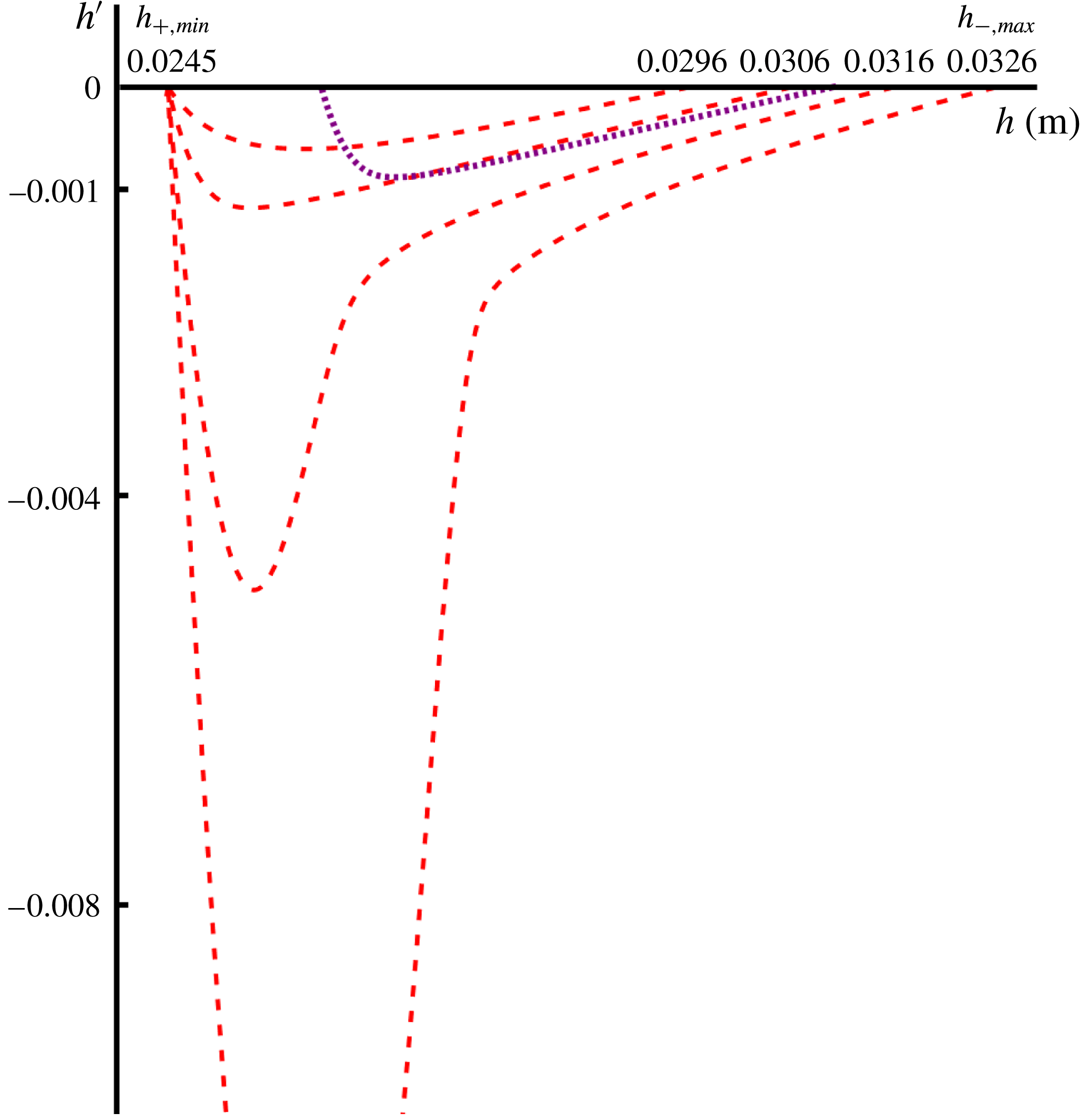
Various trajectories in the
 $(h,h^{\prime })$
plane for a series of monoclinal waves in which the low plateau is kept fixed at its smallest possible (non-static) level
 $h_{+}=h_{+,min}(\unicode[STIX]{x1D701})$
for the given inclination angle
 $\unicode[STIX]{x1D701}=33.3^{\circ }$
, for several increasing values of
 $h_{-}$
. The trajectories are seen to acquire a pronounced dip (i.e. a relatively steep wave front around the inflection point) when the high plateau is close to the upper threshold level
 $h_{-}=h_{-,max}(\unicode[STIX]{x1D701})$
. This is a manifestation of the Kapitza instability that occurs when
 $h_{-}$
exceeds this thickness. The dotted curve running from
 $h=0.026$
m to
 $h=0.031$
m (reproduced from figure 8) has been inserted to facilitate the comparison with figure 8.

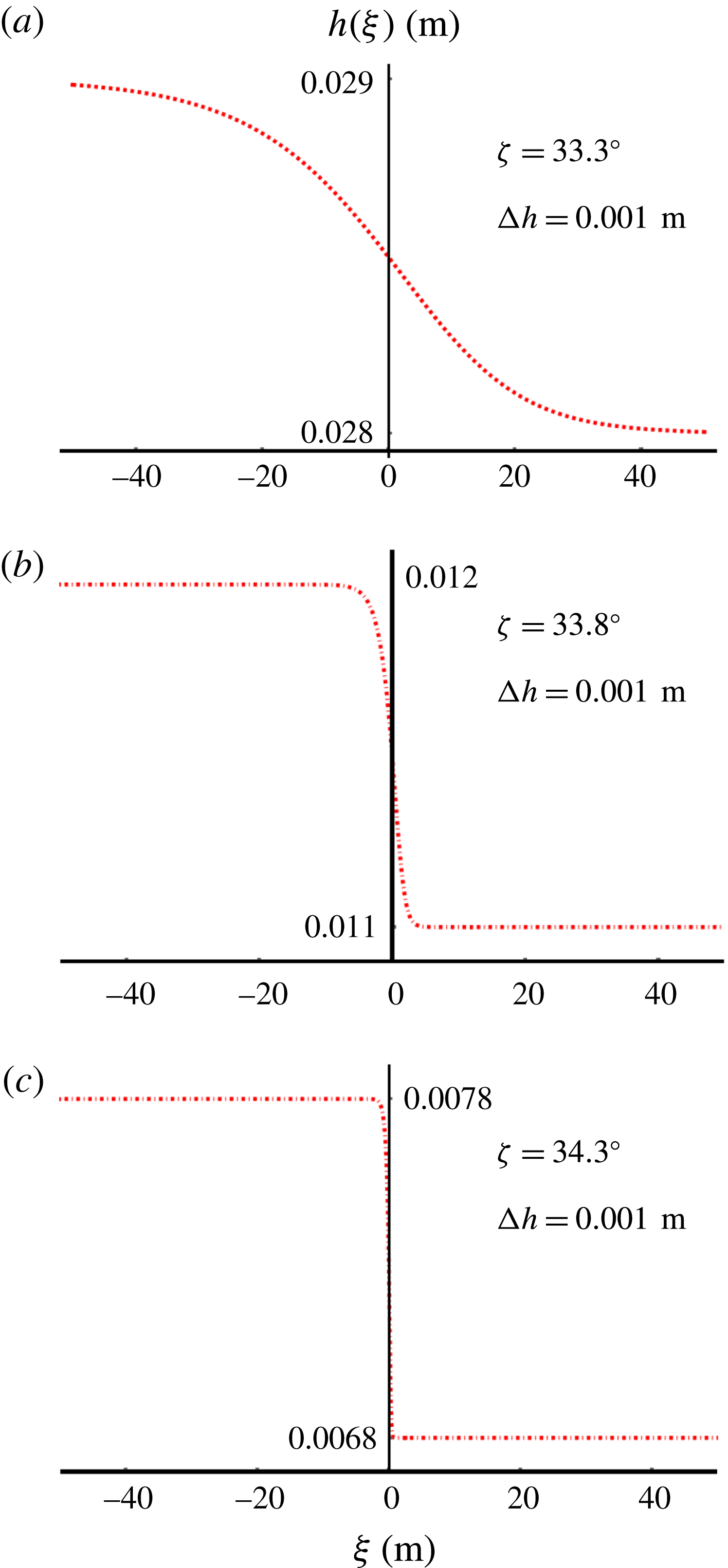
Three monoclinal wave solutions of the second-order ODE (3.4) with the same amplitude
 $\unicode[STIX]{x0394}h=h_{-}-h_{+}=1~\text{mm}$
, on three chutes with different inclinations
 $\unicode[STIX]{x1D701}$
. (a) For the relatively small angle
 $\unicode[STIX]{x1D701}=33.3^{\circ }$
(our standard value) the profile is seen to be very smooth and almost symmetric about
 $h(0)=(h_{-}+h_{+})/2$
. (b) For the slightly larger angle
 $\unicode[STIX]{x1D701}=33.8^{\circ }$
the monoclinal profile is steeper and somewhat less symmetric. (c) As we increase the inclination angle a little further to
 $\unicode[STIX]{x1D701}=34.3^{\circ }$
, we witness a very steep and clearly asymmetric profile. Note that the heights of the plateaus
 $h_{-}$
and
 $h_{+}$
had to be chosen differently for the three depicted waves in order to fall into the stability zone (blank interval) in figure 4.

In order to highlight the value of the slope, we plot
 $h^{\prime }(\unicode[STIX]{x1D709})$
versus
 $h(\unicode[STIX]{x1D709})$
, just as before. Figure 10 shows the result:
As long as the thickness
 $h_{-}$
of the high plateau is sufficiently smaller than the maximally allowed value
 $h_{-,max}(\unicode[STIX]{x1D701})$
, the curves in the
 $(h,h^{\prime })$
plane stay close to the horizontal axis, meaning that the slope
 $h^{\prime }(\unicode[STIX]{x1D709})$
remains relatively small along the entire profile of the monoclinal wave. (This is similar to the behaviour we saw in figure 8, and for easy reference we include that trajectory also in the present plot, as a dotted curve).
However, when the thickness
 $h_{-}$
approaches the threshold value
 $h_{-,max}(\unicode[STIX]{x1D701})$
, the curve develops a pronounced dip, meaning that the slope
 $h^{\prime }(\unicode[STIX]{x1D709})$
now attains large negative values around the inflection point of the profile. That is, the wave acquires a steep front. This is a manifestation of the fact that the system is now only barely able to sustain the balance of forces required for the monoclinal profile. When the thickness of the high plateau is chosen to be exactly equal to the threshold value
 $h_{-,max}(\unicode[STIX]{x1D701})$
, which for the inclination angle
 $\unicode[STIX]{x1D701}=33.3^{\circ }$
lies at 32.6 mm, the dip becomes infinitely deep, corresponding to a vertical wave front. And if
 $h_{-}$
exceeds this value, however marginally, the flowing sheet is no longer able to maintain a monoclinal shape and destabilizes via the Kapitza instability. The granular sheet is then forced to switch to a different wave form, which happens to be that of a roll wave. Thus the dip appearing in the
 $(h,h^{\prime })$
plane as
 $h_{-}\rightarrow h_{-,max}(\unicode[STIX]{x1D701})$
(i.e. the steepening of the wave front) is a precursor of the Kapitza instability.
A second way of producing monoclinal waves with steep fronts is to increase the inclination angle
 $\unicode[STIX]{x1D701}$
of the chute. This is illustrated in figure 11. Here we see three monoclinal solutions of the full viscous ODE (3.4), this time with the same amplitude
 $\unicode[STIX]{x0394}h=h_{-}-h_{+}=1~\text{mm}$
but on chutes with different angles
 $\unicode[STIX]{x1D701}$
. The first one, propagating on a chute with our standard angle
 $\unicode[STIX]{x1D701}=33.3^{\circ }$
, is seen to be smooth and almost symmetric about the central point at
 $\unicode[STIX]{x1D709}=0$
. The second profile, for
 $\unicode[STIX]{x1D701}=33.8^{\circ }$
, is already considerably steeper. For the third profile, on a chute with inclination angle
 $\unicode[STIX]{x1D701}=34.3^{\circ }$
, the wave is again steeper and moreover clearly asymmetric. We will come back to this in § 4, where we will show that in the steep region the viscous-like term plays an important role in keeping the slope finite; without viscosity, the wave front would become infinitely steep beyond a certain critical value of
 $\unicode[STIX]{x1D701}$
.
3.4 A special monoclinal wave: an avalanche on an empty chute
An interesting variety of the monoclinal wave is found when we set
 $h_{+}=0$
. In this special case, the ODE (3.4) can be solved analytically. The solution describes an avalanche front propagating on an empty chute, experimentally sighted and analysed by Pouliquen (Reference Pouliquen1999) and further studied by Gray & Ancey (Reference Gray and Ancey2009).
To find the analytical expression for this avalanche front, we first note that
 $K=0$
for
 $h_{+}=0$
(i.e. the flux in the co-moving frame vanishes), as can be deduced from (3.2) by setting
 $h=h_{+}=0$
. Then, the viscous (3.4) and its inviscid approximation equation (3.6) both reduce to the same first-order ODE:
 $$\begin{eqnarray}\frac{\text{d}h}{\text{d}\unicode[STIX]{x1D709}}=(\tan \unicode[STIX]{x1D701}_{2}-\tan \unicode[STIX]{x1D701}_{1})\left(\frac{1}{1+\unicode[STIX]{x1D6FE}(\unicode[STIX]{x1D701})}-\frac{1}{1+\unicode[STIX]{x1D6FE}(\unicode[STIX]{x1D701})(h/h_{-})^{3/2}}\right),\end{eqnarray}$$
which can also conveniently be written in non-dimensional form, with the height
 $h$
normalized to
 $\widetilde{h}=h/h_{-}$
and the travelling wave coordinate to
 $\widetilde{\unicode[STIX]{x1D709}}=(\tan \unicode[STIX]{x1D701}_{2}-\tan \unicode[STIX]{x1D701}_{1})\unicode[STIX]{x1D709}/h_{-}$
:
 $$\begin{eqnarray}\frac{\text{d}\widetilde{h}}{\text{d}\widetilde{\unicode[STIX]{x1D709}}}=\frac{1}{1+\unicode[STIX]{x1D6FE}(\unicode[STIX]{x1D701})}-\frac{1}{1+\unicode[STIX]{x1D6FE}(\unicode[STIX]{x1D701})\widetilde{h}^{3/2}}.\end{eqnarray}$$
This first-order ODE can be solved analytically to give
 $\widetilde{\unicode[STIX]{x1D709}}$
as a function of
 $\widetilde{h}$
:
 $$\begin{eqnarray}\displaystyle \widetilde{\unicode[STIX]{x1D709}}+C & = & \displaystyle \frac{1+\unicode[STIX]{x1D6FE}(\unicode[STIX]{x1D701})}{3\unicode[STIX]{x1D6FE}(\unicode[STIX]{x1D701})}\left\{3\unicode[STIX]{x1D6FE}(\unicode[STIX]{x1D701})\widetilde{h}+2\sqrt{3}(1+\unicode[STIX]{x1D6FE}(\unicode[STIX]{x1D701}))\arctan \left(\frac{1+2\sqrt{\widetilde{h}}}{\sqrt{3}}\right)\right.\nonumber\\ \displaystyle & & \displaystyle +\left.(1+\unicode[STIX]{x1D6FE}(\unicode[STIX]{x1D701}))\ln \left(\frac{1-2\sqrt{\widetilde{h}}+\widetilde{h}}{1+\sqrt{\widetilde{h}}+\widetilde{h}}\right)\right\},\end{eqnarray}$$
where the integration constant
 $C$
may be chosen in such a way that the wave front is located at
 $\widetilde{\unicode[STIX]{x1D709}}=0$
, i.e.
 $C=\unicode[STIX]{x03C0}(1+\unicode[STIX]{x1D6FE}(\unicode[STIX]{x1D701}))^{2}/3\sqrt{3}\unicode[STIX]{x1D6FE}(\unicode[STIX]{x1D701})$
. The above solution (3.12), with the axes arranged such as to show
 $\widetilde{h}$
as a function of
 $\widetilde{\unicode[STIX]{x1D709}}$
, is depicted in figure 12 for three different inclination angles
 $\unicode[STIX]{x1D701}$
.
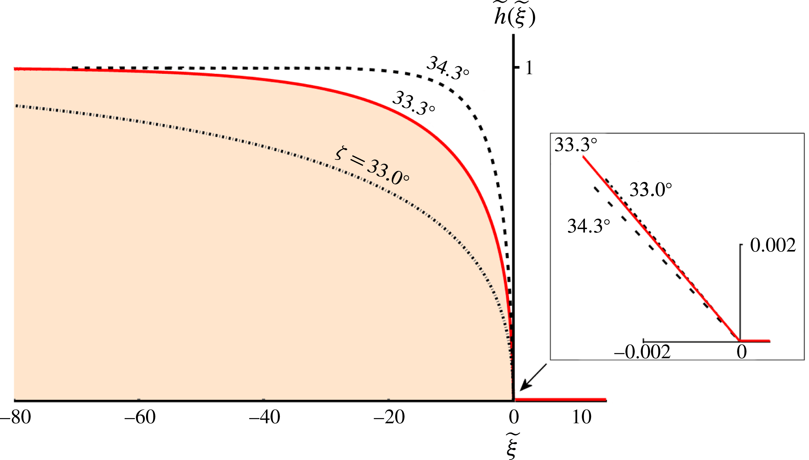
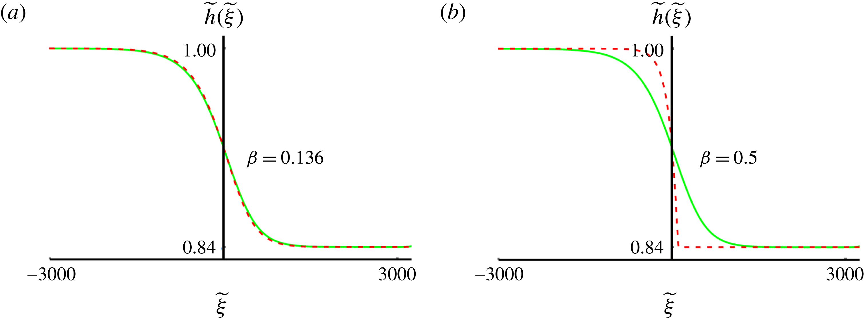
A monoclinal wave (in non-dimensionalized coordinates) propagating on an empty chute, i.e. an avalanche front similar to the one observed and studied by Pouliquen (Reference Pouliquen1999) and Gray & Ancey (Reference Gray and Ancey2009). It is a special solution for
 $h_{+}=0$
of the second-order ODE (3.4) for travelling monoclinal waves. Its analytical form for
 $\widetilde{\unicode[STIX]{x1D709}}\leqslant 0$
is given by (3.12), while for
 $\widetilde{\unicode[STIX]{x1D709}}>0$
we simply impose
 $\widetilde{h}(\widetilde{\unicode[STIX]{x1D709}})=\widetilde{h}_{+}=0$
. The three depicted avalanche fronts correspond to chute with inclination angles
 $\unicode[STIX]{x1D701}=33.0^{\circ }$
,
 $33.3^{\circ }$
and
 $34.3^{\circ }$
, respectively. Close to
 $\widetilde{\unicode[STIX]{x1D709}}=0$
the three curves cross each other and the inset shows that the slope at the origin,
 $\widetilde{h}^{\prime }(0)=-\unicode[STIX]{x1D6FE}(\unicode[STIX]{x1D701})/(1+\unicode[STIX]{x1D6FE}(\unicode[STIX]{x1D701}))$
, is largest for the avalanche on the chute with the smallest inclination angle.

Just as for the monoclinal waves of figure 11, the avalanche front is seen (on the scale of the main figure) to become steeper with increasing
 $\unicode[STIX]{x1D701}$
. There is however an interesting twist in the tail here: the curves attain their maximal steepness at
 $\widetilde{\unicode[STIX]{x1D709}}=0$
, where
 $\text{d}\widetilde{h}/\text{d}\widetilde{\unicode[STIX]{x1D709}}=-\unicode[STIX]{x1D6FE}(\unicode[STIX]{x1D701})/(1+\unicode[STIX]{x1D6FE}(\unicode[STIX]{x1D701}))$
, as can be inferred from (3.11) for
 $\widetilde{h}=0$
. This local slope is actually steepest for
 $\unicode[STIX]{x1D701}\rightarrow \unicode[STIX]{x1D701}_{1}$
(where it approaches
 $-1$
) and goes to zero in the limit for
 $\unicode[STIX]{x1D701}\rightarrow \unicode[STIX]{x1D701}_{2}$
. This reversal of affairs is illustrated in the inset of figure 11. It is only somewhat further away from
 $\widetilde{\unicode[STIX]{x1D709}}=0$
that the curves cross each other and the global picture emerges, with the curve for the largest
 $\unicode[STIX]{x1D701}$
having the steepest slope, complying with the usual behaviour of monoclinal waves.
We note that (3.12), previously derived by Gray & Ancey (Reference Gray and Ancey2009), is the granular analogue of the well-known Bresse solution for ‘gradually varied flow’ in water channels (Bresse Reference Bresse1860; Rouse & Ince Reference Rouse and Ince1963; Jan Reference Jan2014). Since it is a solution of (3.4), it may be recognized as being a special member of the family of travelling granular monoclinal waves, with the distinctive feature that its lower plateau is non-existent (
 $\widetilde{h}_{+}=0$
). For the upper plateau the Froude number must lie in the interval
 $\unicode[STIX]{x1D6FD}<Fr<2/3$
as usual, whereas the Froude number for the lower plateau (i.e. the empty part of the chute) is simply undefined. The corresponding speed of the avalanche is given by:
 $$\begin{eqnarray}c_{ava}=\frac{h_{-}\bar{u}_{-}-h_{+}\bar{u}_{+}}{h_{-}-h_{+}}=\bar{u}_{-},\quad \text{since }h_{+}=0.\end{eqnarray}$$
Similar travelling front profiles for granular flows were analysed by others (Pudasaini Reference Pudasaini2011; Takahashi Reference Takahashi2014; Saingier, Deboeuf & Lagrée Reference Saingier, Deboeuf and Lagrée2016; Lagrée et al.
Reference Lagrée, Saingier, Deboeuf, Staron, Popinet, Radjai, Nezamabadi, Luding and Delenne2017). Pudasaini in 2011, studying a model for debris avalanches occurring in mountainous terrain, was able to derive an analytical solution for the shape of the flow front. Takahashi (Reference Takahashi2014) found very satisfactory agreement with the experimentally measured profile of a stony-type debris flow using a model in which the mass balance was the same as in our analysis but the momentum balance had a different friction law and no viscous-like term. Also Saingier et al. recently analysed a similar model, with the added distinction that the advective term
 $\unicode[STIX]{x2202}_{x}(h\bar{u}^{2})$
was multiplied by a ‘shape factor’ depending on the form of the velocity profile, which for plug flow is equal to unity (Saingier et al.
Reference Saingier, Deboeuf and Lagrée2016; Lagrée et al.
Reference Lagrée, Saingier, Deboeuf, Staron, Popinet, Radjai, Nezamabadi, Luding and Delenne2017). Despite the differences of these models from the system considered here, the analytical solutions obtained by the above authors are reminiscent of (3.12).
4 The inviscid limit
In this section we investigate the region of validity of the inviscid description. This will give us several new insights into the nature of the monoclinal wave and, in particular, we will gain a clear picture of the modest yet not unimportant role of viscosity.
We start by casting the inviscid first-order ODE (3.6) into the following form:
 $$\begin{eqnarray}\frac{\text{d}h}{\text{d}\unicode[STIX]{x1D709}}=\frac{\tan \unicode[STIX]{x1D701}-\unicode[STIX]{x1D707}(h)}{1-K^{2}/(g\cos \unicode[STIX]{x1D701}h^{3})}=\frac{N(h)}{D(h)},\end{eqnarray}$$
where the numerator and the denominator appearing on the right-hand side are denoted by
 $N(h)$
and
 $D(h)$
for ease of reference in our analysis. We will study them both in detail.
Starting with the numerator
 $N(h)=\tan \unicode[STIX]{x1D701}-\unicode[STIX]{x1D707}(h)$
, this portrays the competition between gravity and friction (both divided by
 $g\cos \unicode[STIX]{x1D701}$
). This numerator turns out to be negative on the entire interval of heights
 $h_{+}<h<h_{-}$
relevant for the monoclinal wave, and only becomes zero when the wave attains its exact plateau values
 $h_{\pm }$
at
 $\unicode[STIX]{x1D709}\rightarrow \pm \infty$
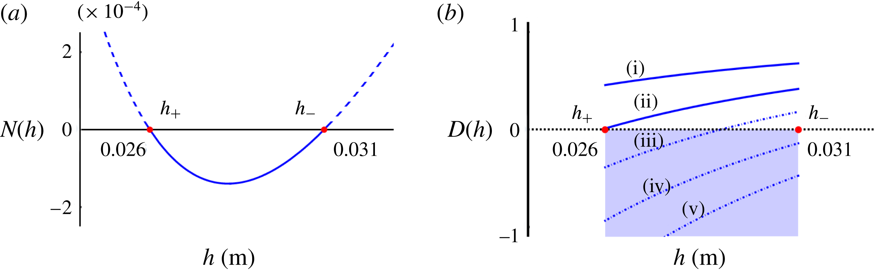
. This is illustrated in figure 13(a). The fact that
 $\unicode[STIX]{x1D707}(h)>\tan \unicode[STIX]{x1D701}$
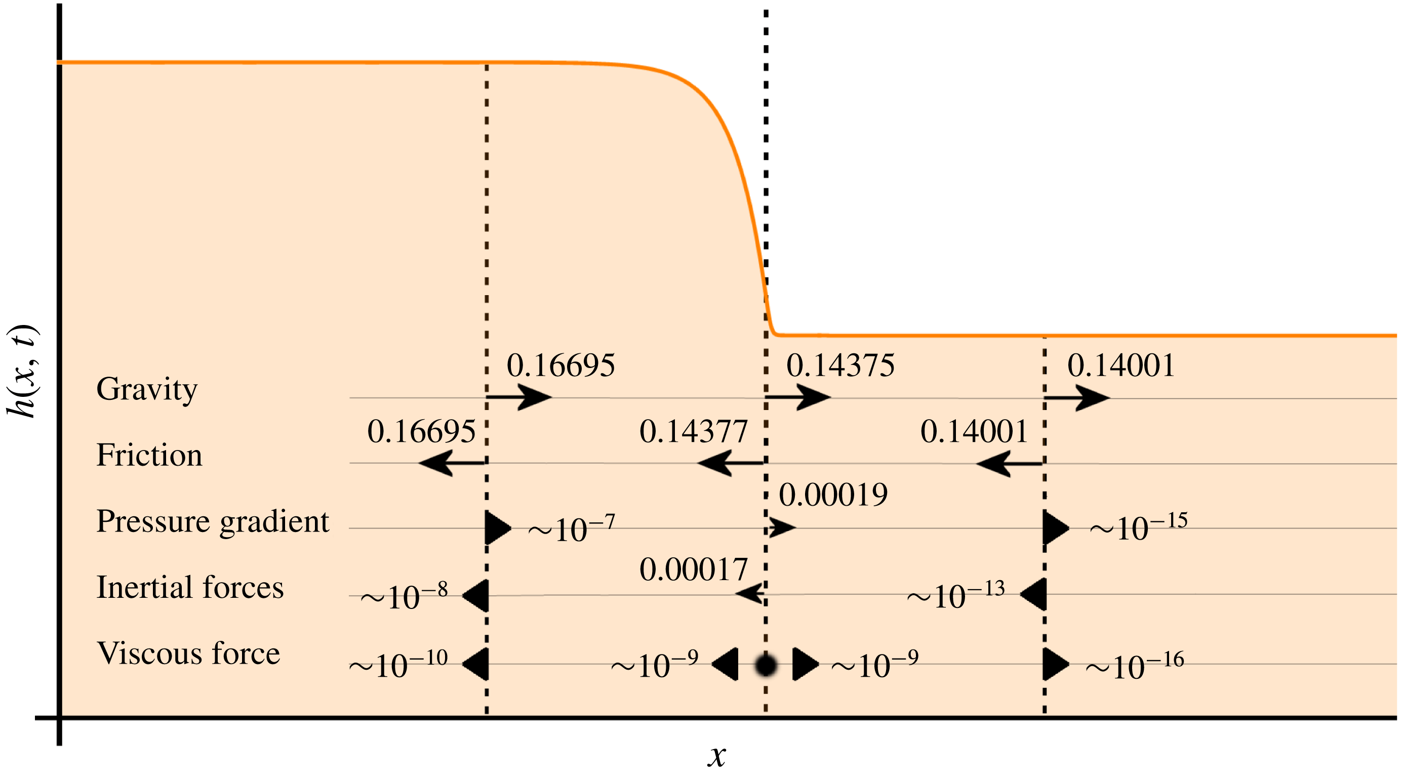
means that in the sloping region of the monoclinal wave the friction force is a little bit stronger than gravity. This calls for additional forces to establish the balance within the wave structure, such as inertial forces and the pressure gradient; cf. figure 15. The balance of forces will be further discussed in § 5.
(a) The numerator
 $N(h)$
of (4.1) is negative on the whole interval
 $h_{+}<h<h_{-}$
, i.e. for all heights relevant for monoclinal waves. Here
 $N(h)$
is depicted for the inclination angle
 $\unicode[STIX]{x1D701}=33.3^{\circ }$
used throughout, cf. figure 4. (b) The denominator
 $D(h)$
of (4.1) is an increasing function of
 $h$
on the same interval. We distinguish three regimes: (i, ii) for
 $\unicode[STIX]{x1D701}_{1}<\unicode[STIX]{x1D701}<\unicode[STIX]{x1D701}_{A}$
(solid blue lines)
 $D(h)$
is everywhere positive and hence
 $\text{d}h/\text{d}\unicode[STIX]{x1D709}<0$
according to (4.1); this corresponds to continually descending monoclinal waves like those shown in figure 9. (iii) For
 $\unicode[STIX]{x1D701}_{A}<\unicode[STIX]{x1D701}<\unicode[STIX]{x1D701}_{B}$
(dash-dotted line)
 $D(h)$
goes through zero at some intermediate height in the relevant interval, giving an infinitely steep slope, i.e. a singularity. (iv, v) For
 $\unicode[STIX]{x1D701}>\unicode[STIX]{x1D701}_{B}$
(dash-dotted) the denominator is everywhere negative, so that
 $\text{d}h/\text{d}\unicode[STIX]{x1D709}>0$
and hence the profile
 $h(\unicode[STIX]{x1D709})$
is now continually rising. This does not correspond to a stable travelling waveform however, as explained in the text.

Also the denominator
 $D(h)$
has a direct physical interpretation. With
 $K=h(c-\bar{u})$
, the term
 $K^{2}/(g\cos \unicode[STIX]{x1D701}h^{3})$
can also be written as:
 $$\begin{eqnarray}\frac{K^{2}}{g\cos \unicode[STIX]{x1D701}h^{3}}=\left(\frac{|\bar{u}-c|}{\sqrt{g\cos \unicode[STIX]{x1D701}h}}\right)^{2}=Fr_{co}^{2},\end{eqnarray}$$
where
 $Fr_{co}=Fr_{co}(h)$
is the Froude number measured in the co-moving frame. In other words:
 $$\begin{eqnarray}D(h)=1-\frac{K^{2}}{g\cos \unicode[STIX]{x1D701}h^{3}}=1-Fr_{co}^{2}(h).\end{eqnarray}$$
This means that the denominator keeps track of the Froude number in the co-moving frame along the monoclinal profile. As noted before,
 $\bar{u}$
is everywhere smaller than the wave speed
 $c$
, with
 $\bar{u}-c$
rising from its most negative value at the low plateau
 $h=h_{+}$
to a less negative value at the high plateau
 $h=h_{-}$
. So in the co-moving frame the flow is everywhere upstream and
 $Fr_{co}(h)=|\bar{u}-c|/\sqrt{g\cos \unicode[STIX]{x1D701}h}$
decreases with growing
 $h$
. Consequently, the denominator
 $D(h)=1-Fr_{co}^{2}(h)$
is an increasing function of
 $h$
, as depicted in figure 13(b).
In the framework of the inviscid approximation, the denominator
 $D(h)$
should never become zero, since a root of
 $D(h)$
implies that the profile attains an infinitely steep slope. In the full viscous theory such a thing will be prevented by the viscous-like term but in the absence of viscosity it is a situation arising inevitably when the amplitude
 $\unicode[STIX]{x0394}h=h_{-}-h_{+}$
or the inclination angle
 $\unicode[STIX]{x1D701}$
exceed a critical value.
More specifically, if the inclination angle of the chute lies between
 $\unicode[STIX]{x1D701}_{1}$
and a threshold angle
 $\unicode[STIX]{x1D701}_{A}$
, the solution of the inviscid (4.1) faithfully gives a monotonically decreasing monoclinal profile, just as in figure 9 (blue solid lines). In this regime, for
 $\unicode[STIX]{x1D701}_{1}<\unicode[STIX]{x1D701}<\unicode[STIX]{x1D701}_{A}$
, the numerator of (4.1) is negative while the denominator is positive, and hence their ratio (i.e. the slope
 $\text{d}h/\text{d}\unicode[STIX]{x1D709}$
of the wave) is negative and finite, as it should be.
The threshold angle
 $\unicode[STIX]{x1D701}_{A}$
is reached when the denominator
 $D(h)$
of (4.1) becomes zero for the first time. This happens at
 $h=h_{+}$
, since
 $D(h)$
is an increasing function of
 $h$
, so the condition for the threshold angle becomes:
 $D(h_{+})=1-K^{2}/(g\cos \unicode[STIX]{x1D701}_{A}h_{+}^{3})=0$
. Noting that also the volumetric flux
 $K$
contains the angle
 $\unicode[STIX]{x1D701}_{A}$
, see (3.8), and solving for
 $\unicode[STIX]{x1D701}_{A}$
we find:
 $$\begin{eqnarray}\unicode[STIX]{x1D701}_{A}=\text{arctan}\left(\frac{f(h_{-},h_{+})\tan \unicode[STIX]{x1D701}_{1}+\tan \unicode[STIX]{x1D701}_{2}}{f(h_{-},h_{+})+1}\right),\end{eqnarray}$$
with
 $$\begin{eqnarray}f(h_{-},h_{+})=\frac{\unicode[STIX]{x1D6FD}h_{+}}{{\mathcal{L}}}\left[\frac{1-(h_{-}/h_{+})^{5/2}}{1-(h_{-}/h_{+})}-1\right].\end{eqnarray}$$
The above analysis is illustrated in figure 14, which shows the profiles of the monoclinal wave solutions (both for the inviscid approximation and for the viscous case) for three successive values of the inclination angle
 $\unicode[STIX]{x1D701}$
. All three profiles have the same amplitude
 $\unicode[STIX]{x0394}h=5.0~\text{mm}$
with
 $h_{-}=31.0~\text{mm}$
and
 $h_{+}=26.0~\text{mm}$
. In the first profile, for
 $\unicode[STIX]{x1D701}=33.280^{\circ }$
, we see that the inviscid and viscous models give indistinguishable results. As we increase the inclination angle, however, the profile becomes steeper. For
 $\unicode[STIX]{x1D701}=33.300^{\circ }$
(figure 14
b) we see that the inviscid approximation starts to deviate, which becomes visible by enlarging the critical zone around the inflection point, although the steepness is still everywhere finite. In (c) we show what happens when
 $\unicode[STIX]{x1D701}$
exceeds the threshold value
 $\unicode[STIX]{x1D701}_{A}$
(equal to
 $33.3023^{\circ }$
for the given parameter values, cf. (4.4)–(4.5)): at
 $\unicode[STIX]{x1D701}=33.305^{\circ }$
the inviscid approximation acquires an infinitely steep slope around the former inflection point. This point is indicated by the solid black dot. The singularity is an artefact caused by ignoring the diffusive effects. Indeed, the viscous solution (red dashed line) goes on unhindered; its slope always remains finite owing to the smoothing action of the viscous-like term.
Monoclinal wave solutions, both from the inviscid approximation (blue solid lines) and the full viscous model (red dashed lines), for three values of the inclination angle
 $\unicode[STIX]{x1D701}$
. All three profiles have the same plateau heights
 $h_{-}$
and
 $h_{+}$
. The close ups to the right of each figure show the critical region where the profile connects to the lower plateau. (a) For
 $\unicode[STIX]{x1D701}=33.280^{\circ }$
, the inviscid and viscous solutions are seen to match perfectly. (b) For
 $\unicode[STIX]{x1D701}=33.300^{\circ }$
the profile becomes steeper and the inviscid approximation starts to deviate visibly from the viscous case, in the neighbourhood of the inflection point. (c) For
 $\unicode[STIX]{x1D701}=33.305^{\circ }$
, beyond the threshold value
 $\unicode[STIX]{x1D701}_{A}=33.3023^{\circ }$
given by (4.4)–(4.5), the slope of the inviscid approximation becomes infinitely steep at a certain point in the aforementioned neighbourhood, marked by the solid black dot. Meanwhile, the viscous solution (red dashed line) continues unaffected, since it is protected from becoming arbitrarily steep by the smoothing action of the viscous-like term.

Balance of forces in a fully ripened granular monoclinal wave, at three points along its profile. The magnitude and direction of the contributing forces is everywhere such that the resulting net force is zero. The dominant two forces along the entire length of the profile are gravity and friction. In the shock zone, due to the variations in thickness and depth-averaged velocity, also the other forces come into play. The pressure gradient and the inertial forces are seen to be approximately of the same order of magnitude, whereas the viscous force is by far the smallest of all. The latter only rears its head in the immediate neighbourhood of the inflection point, which lies very close to the vertical dashed line in the centre of this figure (see text). NB: Since the ‘forces’ we are working with are depth-integrated forces per unit volume, and divided by the constant density, the numbers in this figure are measured in
 $\text{m}^{2}~\text{s}^{-2}$
.

It is interesting to note that the point
 $h=h_{\ast }$
where the denominator
 $D(h)$
becomes zero corresponds to critical flow conditions in the co-moving frame. From (4.3) it is seen that
 $D(h_{\ast })=0$
corresponds to
 $Fr_{co}(h_{\ast })=|\bar{u}-c|/\sqrt{g\cos \unicode[STIX]{x1D701}h}=1$
. In the thin regions of the profile, to the right of the point where
 $h=h_{\ast }$
, the upstream flow as viewed in the co-moving frame is supercritical or torrential (
 $Fr_{co}>1$
); in the thicker regions to the left of this point it is subcritical or fluvial (
 $Fr_{co}<1$
).
In the context of the inviscid theory, these two flow regimes must be connected via a discontinuous jump satisfying the Rankine–Hugoniot shock conditions. For water, the method for constructing such a jump has been described by Whitham (Reference Whitham1974), see figure 3.9 and the associated discussion of the monoclinal flood wave with an inner discontinuity; the same method is also applicable to the granular flows considered here, with the relevant Rankine–Hugoniot conditions for a granular jump having been derived by Gray & Cui (Reference Gray and Cui2007). The introduction of the viscous-like term, however, both in the case of water (Needham & Merkin Reference Needham and Merkin1984) and in the case of granular flows (Gray & Edwards Reference Gray and Edwards2014), has rendered this ingenious remedy of the singularity unnecessary: thanks to the viscous-like term the slope
 $\text{d}h/\text{d}\unicode[STIX]{x1D709}$
always remains finite and hence no singularity occurs. In fact, this is the precise vocation of the viscous-like term. It plays a role only in this particular kind of situation, and only locally, but then it is absolutely indispensable.
The threshold value
 $\unicode[STIX]{x1D701}_{A}$
given by (4.4)–(4.5) – when
 $D(h)$
acquires a root – marks the end of the region of validity of the inviscid approximation, so from a practical point of view one might stop here. Nonetheless, it is instructive to explore this approximation also for inclination angles beyond
 $\unicode[STIX]{x1D701}_{A}$
, not merely out of mathematical curiosity but mainly in order to see what kind of unphysical situations would arise in the absence of the viscous term. Or, put differently, to see why the viscous-like term was such a necessary addition to the momentum balance.
For inclination angles
 $\unicode[STIX]{x1D701}_{A}<\unicode[STIX]{x1D701}<\unicode[STIX]{x1D701}_{B}$
(where
 $\unicode[STIX]{x1D701}_{B}<\unicode[STIX]{x1D701}_{2}$
is a second critical angle), the denominator
 $D(h)$
vanishes for a certain
 $h=h_{d}$
on the interval
 $[h_{+},h_{-}]$
, yielding an infinite negative slope
 $\text{d}h(\unicode[STIX]{x1D709})/\text{d}\unicode[STIX]{x1D709}$
. The numerical scheme breaks down at this point and is no longer able to link the monoclinal profile to the lower plateau. (This second critical angle
 $\unicode[STIX]{x1D701}_{B}$
can be calculated from the condition
 $D(h_{-})=0$
, giving an expression analogous to (4.4) with
 $h_{-}$
and
 $h_{+}$
interchanged:
 $\unicode[STIX]{x1D701}_{B}=\text{arctan}\{(f(h_{+},h_{-})\tan \unicode[STIX]{x1D701}_{1}+\tan \unicode[STIX]{x1D701}_{2})/(f(h_{+},h_{-})+1)\}$
.)
For inclination angles
 $\unicode[STIX]{x1D701}>\unicode[STIX]{x1D701}_{B}$
, things are mathematically sound again, but not physically. Now both the numerator and the denominator of (4.1) are negative, leading to a positive
 $\text{d}h/\text{d}\unicode[STIX]{x1D709}$
, i.e. a monotonously rising profile. Such an inverse monoclinal wave cannot remain intact, however, since its front (high plateau) travels faster than its rear (low plateau), meaning that the profile expands with time and degenerates to a perpetually flattening structure joining two faraway regions with heights
 $h_{-}$
and
 $h_{+}$
.
The mathematical source of this unrealistic prediction of the first-order ODE (4.1) can be traced back to the fact that this equation admits only one boundary condition, whereas the full problem expressed by the second-order ODE (3.4) requires two such conditions. In the solution of the latter, we specify both
 $h(0)$
and the slope
 $h^{\prime }(0)$
, whereas in the inviscid case we cannot prescribe the second one regarding the slope. So the physical restriction that
 $h^{\prime }(0)$
must be negative and finite (in order to correspond to the descending structure of the monoclinal wave) cannot be imposed as a boundary condition on the first-order ODE.
In conclusion, the inviscid approximation expressed by the first-order ODE (4.1) is valid in the truncated interval
 $\unicode[STIX]{x1D701}_{1}<\unicode[STIX]{x1D701}<\unicode[STIX]{x1D701}_{A}$
. Beyond this interval one has to use the full, viscous second-order ODE (3.4) to get physically meaningful solutions.
5 Balance of forces
Further insight in the physics behind the granular monoclinal wave can be gained by an analysis of the balance of forces responsible for its formation and stability. Some terms in the governing equations tend to steepen the wave front, other terms tend to flatten it, and it is only thanks to a balance between these opposing forces that the wave can propagate without change of shape.
The forces featuring in the momentum balance (2.3) are gravity, the pressure gradient, friction and the viscous force on the right-hand side. Just as before, ‘force’ in our discussion here stands for ‘depth-integrated force per unit volume divided by the constant density of the sheet’. The inertial terms on the left-hand side represent the acceleration field within the granular sheet; by transferring them to the right-hand side (with the associated change of sign) these same terms can be interpreted as forces working in the opposite direction. This transfer is analogous to that of an accelerating car, where the (forward) acceleration is experienced by the passengers as a backward force pushing them against their seats. In figure 15 we present the balance of forces within the granular sheet at three different positions
 $x$
along its monoclinal profile. For the purpose of this figure the inertial terms have indeed been transferred to the right-hand side of (2.3) where the forces reside.
The leftmost position in figure 15 represents the high plateau, where the sheet is flowing uniformly with height
 $h_{-}$
and depth-averaged velocity
 $\bar{u}_{-}$
. Likewise, the rightmost position represents the uniform flow of the low plateau with
 $h_{+}$
and
 $\bar{u}_{+}$
. At these two positions, the only forces that have an appreciable magnitude are gravity and friction. Indeed, when the height and velocity become exactly constant (as they do for
 $x\rightarrow \pm \infty$
), all derivatives in the momentum balance vanish; in this limit gravity and friction are the only non-zero forces, which must necessarily balance each other. See also our discussion of the uniform flow conditions in § 2.2.
In the central position, chosen to lie very close to the inflection point of the wave, gravity and friction are still the dominant forces by far, yet also the other forces have come into play owing to the fact that the various derivatives of
 $h$
and
 $\bar{u}$
deviate substantially from zero. The pressure gradient
 $-\unicode[STIX]{x2202}_{x}((1/2)gh^{2}\cos \unicode[STIX]{x1D701})$
produces a force acting towards the direction of diminishing height, which for the given profile is downstream. The inertial forces are slightly more involved, because
 $\unicode[STIX]{x2202}(h\bar{u})/\unicode[STIX]{x2202}t$
is positive (an observer standing on the chute experiences a flood wave of sand with both
 $h$
and
 $\bar{u}$
increasing with time) while
 $\unicode[STIX]{x2202}(h\bar{u}^{2})/\unicode[STIX]{x2202}x$
is negative (since the same observer always sees the profiles of
 $h$
and
 $\bar{u}^{2}$
having a negative slope in the downstream direction); the former is approximately twice as large as the latter, so the net acceleration
 $\unicode[STIX]{x2202}(h\bar{u})/\unicode[STIX]{x2202}t+\unicode[STIX]{x2202}(h\bar{u}^{2})/\unicode[STIX]{x2202}x$
is in the positive downstream direction. Transferred to the right-hand side and hence interpreted as a force, this acceleration is experienced by the granular particles (just as in the analogy with the car passengers) as an inertial force in the upstream direction.
As for the viscous force,
 $\unicode[STIX]{x2202}_{x}(\unicode[STIX]{x1D708}(\unicode[STIX]{x1D701})h^{3/2}\unicode[STIX]{x2202}_{x}\bar{u})$
, we find that it changes sign at a certain point along the shock front. In (3.4) we already found that in the fully ripened state of the monoclinal wave, the viscous term assumes the form:
 $\unicode[STIX]{x1D708}K[h^{-3/2}h^{\prime \prime }-(1/2)h^{-5/2}(h^{\prime })^{2}]$
. The latter expression goes through zero at the point
 $\unicode[STIX]{x1D709}=\unicode[STIX]{x1D709}_{V}$
where
 $h^{\prime \prime }=(1/2)h^{-1}(h^{\prime })^{2}$
, which is positive; hence the point
 $\unicode[STIX]{x1D709}_{V}$
lies to the right of the inflection point. The position
 $\unicode[STIX]{x1D709}=\unicode[STIX]{x1D709}_{V}$
corresponds to the central line of figure 15. In practice, it lies extremely close to the inflection point. Immediately before and after
 $\unicode[STIX]{x1D709}=\unicode[STIX]{x1D709}_{V}$
the viscous force acquires its maximal amplitude, always such as to point away from
 $\unicode[STIX]{x1D709}_{V}$
. This is the typical behaviour of a viscous (diffusive) force, which tends to smear out the differences in height and thus to flatten the profile. This corroborates the role of this force (discussed in the previous sections) as an emergency defence against excessive steepening of the wave front.
Regarding the relative magnitude of the forces, figure 15 shows that the monoclinal profile is predominantly shaped by a balance between gravity and friction. In the middle region also the other forces play their part, yet they always remain considerably smaller than gravity and friction. The pressure gradient and the inertial forces are smaller by approximately three orders of magnitude, while the viscous force is the smallest of all. Even in the immediate vicinity of the inflection point it is eight orders of magnitude smaller than gravity and friction. Bearing this in mind, we shall leave viscosity out of the discussion of the present section. And for maximum clarity, we shall work with the non-dimensional version of the governing equations.
Our first task is to non-dimensionalize the continuity equation and the inviscid momentum balance. We do this by introducing the following rescalings:
 $h=h_{0}\widetilde{h}$
,
 $\bar{u}=\bar{u}_{0}\widetilde{u}$
,
 $x=h_{0}\widetilde{x}$
and
 $t=(h_{0}/\bar{u}_{0})\widetilde{t}$
, where
 $h_{0}$
is a characteristic thickness, say
 $h_{0}=h_{-}$
(the same choice as in the rescaling of (3.10)), and
 $\bar{u}_{0}=\unicode[STIX]{x1D6FD}({\mathcal{L}}\unicode[STIX]{x1D6FE}(\unicode[STIX]{x1D701}))^{-1}\sqrt{g\cos \unicode[STIX]{x1D701}}h_{0}^{3/2}$
is the constant velocity attained by a granular sheet of uniform thickness
 $h_{0}$
. Note that also the distances in the
 $x$
-direction are scaled with the same characteristic length
 $h_{0}$
; this means that the non-dimensional numbers in this direction become quite large, since the typical distances along the chute are several orders of magnitude larger than the characteristic thickness of the sheet.
With the above substitutions, the continuity equation (2.2) takes the form:
 $$\begin{eqnarray}\frac{\unicode[STIX]{x2202}\widetilde{h}}{\unicode[STIX]{x2202}\widetilde{t}}+\frac{\unicode[STIX]{x2202}}{\unicode[STIX]{x2202}\widetilde{x}}(\widetilde{h}\widetilde{u})=0,\end{eqnarray}$$
so this equation actually remains unaltered after the rescaling. Thanks to the fact that the continuity equation is homogeneous in
 $h$
, the corresponding factors
 $h_{0}$
cancel each other, and the remaining scaling factors simply combine to form unity. Note that for notational elegance we have suppressed the bar in the non-dimensional velocity
 $\widetilde{u}$
; it is understood, however, that this velocity is still depth averaged.
The inviscid momentum balance equation (2.3), with
 $\unicode[STIX]{x1D708}=0$
, takes the following non-dimensional form:
 $$\begin{eqnarray}Fr_{0}^{2}\left(\frac{\unicode[STIX]{x2202}\widetilde{u}}{\unicode[STIX]{x2202}\widetilde{t}}+\widetilde{u}\frac{\unicode[STIX]{x2202}\widetilde{u}}{\unicode[STIX]{x2202}\widetilde{x}}\right)=-\frac{\unicode[STIX]{x2202}\widetilde{h}}{\unicode[STIX]{x2202}\widetilde{x}}+\tan \unicode[STIX]{x1D701}-\tan \unicode[STIX]{x1D701}_{1}-\frac{\tan \unicode[STIX]{x1D701}_{2}-\tan \unicode[STIX]{x1D701}_{1}}{1+\unicode[STIX]{x1D6FE}(\widetilde{h}^{3/2}/\widetilde{u})},\end{eqnarray}$$
where we have made use of the continuity equation in order to eliminate
 $\widetilde{h}$
from the left-hand side, and we have divided by
 $\widetilde{h}$
throughout. We have also inserted the explicit form of the friction law (2.4). The ‘characteristic’ Froude number
 $Fr_{0}=\bar{u}_{0}/\sqrt{gh_{0}\cos \unicode[STIX]{x1D701}}$
compares the aforementioned typical velocity
 $\bar{u}_{0}$
of the sheet with
 $\sqrt{gh_{0}\cos \unicode[STIX]{x1D701}}$
, which is the speed with which small-amplitude gravity waves travel over the free surface of a uniform granular sheet of thickness
 $h_{0}$
. From our discussion in § 2, we know that stable monoclinal waves only occur if the Froude number lies in the interval
 $\unicode[STIX]{x1D6FD}<Fr<2/3$
. Hence also the characteristic value
 $Fr_{0}$
(representing the incoming flow with
 $h_{0}=h_{-}$
) must lie within this regime, which implies that
 $Fr_{0}^{2}$
is necessarily smaller than
 $4/9$
.
In the shock zone, as we have seen, the inertial forces are of the same order of magnitude as the pressure gradient. However, if the experimental set-up is such that the parameter
 $\unicode[STIX]{x1D6FD}$
is small, the Froude number
 $Fr_{0}$
may be chosen close to this small value, in which case the prefactor
 $Fr_{0}^{2}$
of the inertial terms in (5.2) renders them insignificant in comparison to the pressure gradient. For instance, the smooth spherical glass beads used by Pouliquen & Forterre (Reference Pouliquen and Forterre2002) have
 $\unicode[STIX]{x1D6FD}=0.136$
, and in this case monoclinal waves are possible with Froude number as low as
 $Fr_{0}=Fr(h_{-},\bar{u}_{-})>Fr(h_{+},\bar{u}_{+})>0.136$
. Or equivalently,
 $Fr_{0}^{2}>0.0185$
, meaning that the effect of the inertial terms on the left-hand side of (5.2) is seriously weakened. This is the regime of creeping flow. This same regime was examined by Börzsönyi et al. not only for spherical glass beads but also for rough non-spherical grains (Börzsönyi, Hasley & Ecke Reference Börzsönyi, Hasley and Ecke2005).
For creeping granular flow, with viscosity and inertia both playing a minor role, the remaining actors in the balance of forces are (in the order in which they appear on the right-hand side of (5.2)): the pressure gradient, gravity and friction. It is interesting to see how these three forces co-operate to cast the shape of the monoclinal wave in the creeping flow limit. Gravity and friction are – as always – the two dominant forces. The pressure gradient sides with gravity, but since the variations
 $\unicode[STIX]{x2202}\widetilde{h}/\unicode[STIX]{x2202}\widetilde{x}$
remain quite small even in the shock regime (the pressure gradient at its peak is typically three orders of magnitude smaller than gravity or friction, see figure 15) the situation is still reasonable close to that of the uniform flow, requiring only a small correction.
Let us see how we can cast this correction in mathematical language. In the creeping flow limit (i.e. without the inertial terms) and in the absence of viscosity, the momentum balance (5.2) takes the form:
 $$\begin{eqnarray}0=-\frac{\unicode[STIX]{x2202}\widetilde{h}}{\unicode[STIX]{x2202}\widetilde{x}}+\tan \unicode[STIX]{x1D701}-\tan \unicode[STIX]{x1D701}_{1}-\frac{\tan \unicode[STIX]{x1D701}_{2}-\tan \unicode[STIX]{x1D701}_{1}}{1+\unicode[STIX]{x1D6FE}(\unicode[STIX]{x1D701})(\widetilde{h}^{3/2}/\widetilde{u})},\end{eqnarray}$$
from which the following expression for the dimensionless speed
 $\widetilde{u}$
can be extracted:
 $$\begin{eqnarray}\widetilde{u}=\unicode[STIX]{x1D6FE}(\unicode[STIX]{x1D701})\frac{\tan \unicode[STIX]{x1D701}-\tan \unicode[STIX]{x1D701}_{1}-(\unicode[STIX]{x2202}\widetilde{h}/\unicode[STIX]{x2202}\widetilde{x})}{\tan \unicode[STIX]{x1D701}_{2}-\tan \unicode[STIX]{x1D701}+(\unicode[STIX]{x2202}\widetilde{h}/\unicode[STIX]{x2202}\widetilde{x})}\widetilde{h}^{3/2}.\end{eqnarray}$$
Now, taking into account that the slope of the monoclinal wave in this creeping limit is everywhere very mild, we may treat
 $\unicode[STIX]{x2202}\widetilde{h}/\unicode[STIX]{x2202}\widetilde{x}$
as a small parameter and make a series expansion of the right-hand side of the above expression. Then, by keeping only the linear terms in
 $\unicode[STIX]{x2202}\widetilde{h}/\unicode[STIX]{x2202}\widetilde{x}$
we obtain:
 $$\begin{eqnarray}\displaystyle \widetilde{u} & = & \displaystyle \unicode[STIX]{x1D6FE}(\unicode[STIX]{x1D701})\left(\frac{\tan \unicode[STIX]{x1D701}-\tan \unicode[STIX]{x1D701}_{1}}{\tan \unicode[STIX]{x1D701}_{2}-\tan \unicode[STIX]{x1D701}}-\frac{\tan \unicode[STIX]{x1D701}_{2}-\tan \unicode[STIX]{x1D701}_{1}}{(\tan \unicode[STIX]{x1D701}_{2}-\tan \unicode[STIX]{x1D701})^{2}}\frac{\unicode[STIX]{x2202}\widetilde{h}}{\unicode[STIX]{x2202}\widetilde{x}}\right)\widetilde{h}^{3/2}\nonumber\\ \displaystyle & = & \displaystyle \widetilde{h}^{3/2}-\frac{\unicode[STIX]{x1D6FE}(\unicode[STIX]{x1D701})+1}{\tan \unicode[STIX]{x1D701}_{2}-\tan \unicode[STIX]{x1D701}}\frac{\unicode[STIX]{x2202}\widetilde{h}}{\unicode[STIX]{x2202}\widetilde{x}}\widetilde{h}^{3/2},\end{eqnarray}$$
where we have used
 $\unicode[STIX]{x1D6FE}(\unicode[STIX]{x1D701})=(\tan \unicode[STIX]{x1D701}_{2}-\tan \unicode[STIX]{x1D701})/(\tan \unicode[STIX]{x1D701}-\tan \unicode[STIX]{x1D701}_{1})$
, cf. (2.5). The above expression for
 $\widetilde{u}$
is the anticipated correction to the uniform flow relation
 $\widetilde{u}=\widetilde{h}^{3/2}$
. Given that
 $\unicode[STIX]{x2202}\widetilde{h}/\unicode[STIX]{x2202}\widetilde{x}$
is negative, equation (5.5) tells us that a stationary observer, at a fixed position
 $\widetilde{x}=\widetilde{x}_{0}$
along the chute, will see the depth-averaged velocity
 $\widetilde{u}(\widetilde{x}_{0},\widetilde{t})$
grow as the wave passes by. This is exactly the rise in velocity that accompanies the transition from the original low plateau conditions to the high plateau conditions at later times.
Substituting (5.5) back into the non-dimensional continuity equation (5.1), we arrive at the following partial differential equation for
 $\widetilde{h}(\widetilde{x},\widetilde{t})$
:
 $$\begin{eqnarray}\frac{\unicode[STIX]{x2202}\widetilde{h}}{\unicode[STIX]{x2202}\widetilde{t}}+\frac{5}{2}\widetilde{h}^{3/2}\frac{\unicode[STIX]{x2202}\widetilde{h}}{\unicode[STIX]{x2202}\widetilde{x}}=\frac{2}{7}\frac{\unicode[STIX]{x1D6FE}(\unicode[STIX]{x1D701})+1}{\tan \unicode[STIX]{x1D701}_{2}-\tan \unicode[STIX]{x1D701}}\frac{\unicode[STIX]{x2202}^{2}\widetilde{h}^{7/2}}{\unicode[STIX]{x2202}\widetilde{x}^{2}}.\end{eqnarray}$$
This nonlinear wave equation describes, within the creeping flow approximation outlined above, the evolution of a monoclinal wave in granular chute flow. (The monoclinal waves described by (5.6) may be called kinematic, since they are determined from the continuity equation augmented by a closure relation for the depth-averaged velocity. Nonetheless, since this closure relation
 $\widetilde{u}=\widetilde{u}(\widetilde{h},\unicode[STIX]{x2202}\widetilde{h}/\unicode[STIX]{x2202}\widetilde{x})$
is derived from a truncated form of the momentum balance, the waves also carry dynamic features. Therefore, a more apt term for these waves might be ‘quasi-kinematic’.) The time derivative appearing on the left-hand side allows for the existence of a propagating waveform, the shape of which is determined by the competition of two nonlinear effects: (i) steepening of the wave front from the second term on the left-hand side, and (ii) an opposing flattening effect from the nonlinear (slow) diffusion term on the right-hand side. The balance between these two effects is self-regulatory: when the initial slope of the profile is too gentle, the steepening effect will make it sharper up to the point when it is balanced by the slow diffusion, and vice versa.
Interestingly, the slow diffusion in (5.6) does not stem from the viscous-like term (which by its nature would also contribute a flattening effect but was ignored in the above analysis); rather, it originates from the friction force in the granular sheet.
Comparison of the profiles arising from the non-dimensionalized nonlinear wave equation (5.6), green solid lines, with the dimensionless monoclinal solution
 $\widetilde{h}_{full}(\widetilde{\unicode[STIX]{x1D709}})$
of the full second-order ODE (3.4), red dashed lines. The green curves represent the creeping flow approximation, i.e. the shape the monoclinal wave would assume if inertial effects were negligible. (a) For small Froude numbers – which can be attained if the parameter
 $\unicode[STIX]{x1D6FD}$
is chosen sufficiently small, here
 $\unicode[STIX]{x1D6FD}=0.136$
– this is seen to be a very good approximation. The Froude number of the incoming sheet is
 $Fr_{0}=Fr(h_{-},\bar{u}_{-})=0.172$
, while that of the outgoing sheet is
 $Fr(h_{+},\bar{u}_{+})=0.145>\unicode[STIX]{x1D6FD}(=0.136)$
, i.e. still sufficient to keep the granular material flowing. (b) For larger Froude numbers the creeping flow approximation is evidently not accurate, meaning that in this case the inertial terms play a significant role. The incoming and outgoing sheets here have
 $Fr(h_{-},\bar{u}_{-})=0.633$
and
 $Fr(h_{+},\bar{u}_{+})=0.532>\unicode[STIX]{x1D6FD}(=0.5)$
. Note the huge difference between the horizontal and vertical axes, reflecting the fact that the typical length scale of a monoclinal wave in the horizontal direction is several orders of magnitude larger than its height. We use dimensionless coordinates with
 $\widetilde{h}_{-}=1$
as the unit of length.

The above analysis is illustrated in figure 16, where we compare the profile evaluated from the nonlinear wave equation (5.6) (solid green line) with the exact monoclinal wave solution
 $h_{full}(\unicode[STIX]{x1D709})$
, obtained from the second-order ODE (3.4) rescaled to dimensionless units (red dashed line).
The situation of figure 16(a) might be observed in an experiment with the smooth spherical glass beads used by Pouliquen & Forterre (Reference Pouliquen and Forterre2002), for which
 $\unicode[STIX]{x1D6FD}=0.136$
. The depicted monoclinal wave (red dashed line) has
 $Fr_{0}=Fr(h_{-},\bar{u}_{-})=0.172$
and
 $Fr(h_{+},\bar{u}_{+})=0.145$
; the latter value must exceed
 $\unicode[STIX]{x1D6FD}$
to ensure that the sheet keeps flowing. This wave is reproduced perfectly by the creeping flow approximation given by the solid green line, so in this regime of small Froude numbers (5.6) is valid and the aforementioned competition between nonlinear steepening and slow diffusion accurately captures the physics of the monoclinal wave.
As expected, for higher Froude numbers the approximation becomes increasingly poor. This is seen in figure 16(b) for our standard particles with
 $\unicode[STIX]{x1D6FD}=0.5$
, which means that
 $Fr$
should not fall anywhere below
 $0.5$
if we want to see an uninterrupted flow. More precisely, with the inequality equation (2.8), we require:
 $\unicode[STIX]{x1D6FD}=0.5<Fr(h_{+},\bar{u}_{+})<Fr(h_{-},\bar{u}_{-})=Fr_{0}<2/3$
and the monoclinal wave (red dashed line) in figure 16(b) indeed fulfils this condition. Clearly, the creeping flow approximation (solid green line) has lost its accuracy at these Froude numbers, so in this case the inertial terms are not negligible. Indeed, practically the entire deviation seen in figure 16(b) is caused by discarding the inertial terms, since we know that in this regime the deviation caused by ignoring viscosity is only very minor (it would not be visible on the scale of the present figure, as corroborated also by figure 9).
In closing we note that (5.6) bears a marked resemblance to the Burgers equation with diffusion,
 $\unicode[STIX]{x2202}_{t}h+ah\unicode[STIX]{x2202}_{x}h=b\unicode[STIX]{x2202}_{xx}h$
, only with a higher-order nonlinear term on the left-hand side (
 $h^{3/2}\unicode[STIX]{x2202}_{x}h$
instead of
 $h\unicode[STIX]{x2202}_{x}h$
) and a distinctly nonlinear diffusive term on the right-hand side. Indeed, also the Burgers equation is known to have monoclinal wave solutions (Whitham Reference Whitham1974), with the subtle difference that those of the Burgers equation are always fully symmetric with respect to the central point at height
 $(h_{-}+h_{+})/2$
, whereas the monoclinal waves arising from (5.6) can also assume asymmetric shapes. A similar Burgers-like equation was also derived by Börzsönyi et al. (Reference Börzsönyi, Hasley and Ecke2005), yet these authors did not consider monoclinal waves; instead, they concentrated on solutions corresponding to single-humped granular avalanches propagating down an inclined plane.
6 Concluding remarks: a guide to the experimental detection of granular monoclinal waves
In this paper we have studied the formation and evolution of granular monoclinal waves, i.e. travelling shock structures connecting a high plateau (height
 $h=h_{-}$
) to a lower one (
 $h=h_{+}$
) via a monotonically descending profile. Our analysis has been based on a depth-averaged hydrodynamic approach in the spirit of Saint-Venant, with the momentum balance being enriched with a granular friction law (Pouliquen & Forterre Reference Pouliquen and Forterre2002) and a viscous-like term arising from the depth-averaged
 $\unicode[STIX]{x1D707}(I)$
-rheology of the granular sheet (Gray & Edwards Reference Gray and Edwards2014).
As noted in the introduction, this monoclinal wave was the last missing piece from a bigger scheme, namely, to match every waveform of the Saint-Venant equations for water with their granular counterparts. From our analysis it has become clear that stable granular monoclinal waves without stopping regions exist for Froude numbers
 $\unicode[STIX]{x1D6FD}<Fr<2/3$
. Here the lower threshold (
 $Fr=\unicode[STIX]{x1D6FD}$
) is dictated by Pouliquen and Forterre’s frictional law – below this threshold the granular sheet simply comes to a halt – while the upper threshold
 $Fr=2/3$
marks the onset of the Kapitza instability, which destabilizes the characteristic uniform plateaus of the monoclinal wave (as shown in figure 6) and gives rise to granular roll waves instead (Gray & Edwards Reference Gray and Edwards2014; Razis et al.
Reference Razis, Edwards, Gray and van der Weele2014; Edwards & Gray Reference Edwards and Gray2015).
The friction always plays a significant role in the balance of forces within the monoclinal wave. As a matter of fact, in the flat plateaus (away from the actual shock structure) the competition between friction and gravity fully determines the speed of the granular sheet. In the shock itself also the inertial terms, the pressure gradient and viscosity come into play; together all these forces determine the precise shape of the monoclinal profile.
As for the viscous-like term, it turns out that its contribution is significant in the small region close to the front of the monoclinal wave (around its inflection point, where the slope
 $\unicode[STIX]{x2202}h/\unicode[STIX]{x2202}\unicode[STIX]{x1D709}$
is maximal) whenever there is a need to prevent this front from becoming too steep. This is a situation that occurs when the inclination angle
 $\unicode[STIX]{x1D701}$
of the chute is near its maximum value
 $\unicode[STIX]{x1D701}_{2}$
or when the amplitude of the wave
 $\unicode[STIX]{x0394}h=h_{-}-h_{+}$
is close to maximal. For mild inclination angles (close to the minimum value
 $\unicode[STIX]{x1D701}_{1}$
) and for waves of relatively small amplitude, the viscous-like term never really comes into play at all. The monoclinal wave is then well described by the inviscid approximation, as demonstrated in § 3 and worked out further in §§ 4 and 5.
To conclude the paper, we want to comment upon the feasibility of observing granular monoclinal waves in experiments. Bearing in mind that a monoclinal wave is the shock structure assumed by a slowly flowing granular fluid when it has to connect two plateaus of different thickness, one may create it by starting with a uniform base flow (
 $Fr<2/3$
) and then gradually lifting the sluice gate at the entrance of the chute. Provided that the Froude number of the thicker layer is also below
 $2/3$
, one will witness the formation of a monoclinal wave, or at least the tendency of the granular flow to organize itself in a monoclinal-like fashion. The fully ripened form of this waveform can only be anticipated to be observed in long chutes since, as we have seen, the longitudinal length scale is several orders of magnitude larger than the transversal length scale (i.e. the amplitude of the wave). We are however optimistic that it will be possible to detect these waves, albeit in their not fully ripened form, since a special type of monoclinal wave (namely, the granular avalanche front propagating on an empty chute, described in § 3.4) has already been observed.
In order to optimize the chances of experimental detection, one should choose the parameter values such as to make the monoclinal wave as pronounced as possible. There are two different ways of achieving this:
(i) The first method is to enhance its amplitude
 $\unicode[STIX]{x0394}h=h_{-}-h_{+}$
. The maximal amplitude a monoclinal wave can attain occurs when its high plateau is as high as possible
 $[h_{-,max}(\unicode[STIX]{x1D701})=2{\mathcal{L}}\unicode[STIX]{x1D6FE}(\unicode[STIX]{x1D701})/(3\unicode[STIX]{x1D6FD})]$
and its low plateau is as low as possible
 $[h_{+,min}(\unicode[STIX]{x1D701})={\mathcal{L}}\unicode[STIX]{x1D6FE}(\unicode[STIX]{x1D701})]$
, yielding:
 $$\begin{eqnarray}\unicode[STIX]{x0394}h_{max}(\unicode[STIX]{x1D701})=h_{-,max}(\unicode[STIX]{x1D701})-h_{+,min}(\unicode[STIX]{x1D701})={\mathcal{L}}\unicode[STIX]{x1D6FE}(\unicode[STIX]{x1D701})\left(\frac{2}{3\unicode[STIX]{x1D6FD}}-1\right).\end{eqnarray}$$
Thus, we can construct the largest amplitudes for granular materials for which the parameter
 ${\mathcal{L}}$
is large and
 $\unicode[STIX]{x1D6FD}$
is small. Also
 $\unicode[STIX]{x1D6FE}(\unicode[STIX]{x1D701})$
should be large; this is towards the left of the phase diagram of figure 4, i.e. when the inclination angle of the chute is close to its lower bound (
 $\unicode[STIX]{x1D701}\rightarrow \unicode[STIX]{x1D701}_{1}$
).
(ii) The second method is to make the wave front as sharp as possible, and thus easily discernible. This can be done by increasing the inclination angle
 $\unicode[STIX]{x1D701}$
of the chute. One has to bear in mind, however, that any increase in
 $\unicode[STIX]{x1D701}$
(and hence decrease of
 $\unicode[STIX]{x1D6FE}(\unicode[STIX]{x1D701})$
) is accompanied by a decrease of the maximal amplitude
 $\unicode[STIX]{x0394}h_{max}(\unicode[STIX]{x1D701})$
, see (6.1). So in practice one will choose an optimum mix of the two methods, by choosing a material with large
 ${\mathcal{L}}$
and small
 $\unicode[STIX]{x1D6FD}$
, and an inclination angle that is reasonably close to
 $\unicode[STIX]{x1D701}_{1}$
, but at the same time sufficiently far away from
 $\unicode[STIX]{x1D701}_{1}$
to get a well-defined front.
The above adjustment of the parameter values will also have an effect on the ratio between the typical length scales in the longitudinal and transverse directions. Strictly speaking, the longitudinal length scale is infinite by definition (because the precise plateau values
 $h_{-}$
and
 $h_{+}$
are attained only at
 $\unicode[STIX]{x1D709}=-\infty$
and
 $\unicode[STIX]{x1D709}=+\infty$
, respectively); a mechanical analogue of this can be found in the mathematical pendulum swinging from its unstable upright position – via the downward equilibrium – to the upright position again, which can be proven mathematically to take an infinite amount of time. From a practical point of view, however, it is more natural to define the ‘length’ of the monoclinal profile (
 $\unicode[STIX]{x0394}\ell$
) as the length of an interval around the midpoint
 $h(\unicode[STIX]{x1D709}=0)=h_{+}+(1/2)\unicode[STIX]{x0394}h$
stretching towards left and right up to where the profile has saturated to within
 $10$
per cent (say) of the respective plateau values, i.e. to
 $h_{+}+0.9\unicode[STIX]{x0394}h$
and
 $h_{+}+0.1\unicode[STIX]{x0394}h$
respectively. We distinguish two limiting cases:
Two phase diagrams (similar to figure 4) for actual experimental set-ups, with the following parameter values: (a)
 $\unicode[STIX]{x1D6FD}=0.63$
,
 ${\mathcal{L}}=0.44~\text{mm}$
,
 $\unicode[STIX]{x1D701}_{1}=31.1^{\circ }$
and
 $\unicode[STIX]{x1D701}_{2}=47.5^{\circ }$
(Edwards et al.
Reference Edwards, Viroulet, Kokelaar and Gray2017), (b)
 $\unicode[STIX]{x1D6FD}=0.136$
,
 ${\mathcal{L}}=0.65~\text{mm}$
,
 $\unicode[STIX]{x1D701}_{1}=21.0^{\circ }$
and
 $\unicode[STIX]{x1D701}_{2}=30.7^{\circ }$
(Pouliquen & Forterre Reference Pouliquen and Forterre2002). The blank zone corresponding to stable monoclinal waves is very narrow in the first diagram (yet may become wider than depicted here if one takes into account an offset in the flow rule for carborundum, see the main text). The same zone in the second diagram is much wider, giving excellent prospects of detecting monoclinal waves in practice.

(i) If one has a monoclinal wave with a mild slope over its entire length, the profile is nearly symmetric and does (in the interval indicated above) not deviate too much from a straight oblique line. In this case, a reasonable approximation for the aspect ratio of the wave
 $\unicode[STIX]{x0394}h/\unicode[STIX]{x0394}\ell$
is simply the (absolute value of the) slope
 $\text{d}h/\text{d}\unicode[STIX]{x1D709}$
at
 $\unicode[STIX]{x1D709}=0$
. And, since the viscous-like term does not play any significant role in the case of mildly sloping monoclinal profiles, we may use the inviscid expression (3.6) to evaluate the slope in question. Its value is typically of the order of
 $10^{-4}$
, as can be inferred for instance from figure 11(a). This implies that (for symmetric monoclinal waves) the length scales in the longitudinal and transverse directions are separated by four orders of magnitude, or equivalently, the aspect ratio
 $\unicode[STIX]{x0394}h/\unicode[STIX]{x0394}\ell$
is of the order of
 $10^{-4}$
.
(ii) If one chooses the inclination angle of the chute such that the front is relatively sharp, the length scales come closer together, although they remain well separated by approximately three orders of magnitude. A representative example of this situation can be found in figure 11(c). In this case the profile (at the left-hand side) crosses the level
 $h_{+}+0.9\unicode[STIX]{x0394}h$
at about
 $\unicode[STIX]{x1D709}=-0.73~\text{m}$
and at the right-hand side it goes through
 $h_{+}+0.1\unicode[STIX]{x0394}h$
at about
 $\unicode[STIX]{x1D709}=0.20~\text{m}$
, amounting to a length
 $\unicode[STIX]{x0394}\ell$
of slightly less than 1 m. Given that the amplitude of the wave is
 $\unicode[STIX]{x0394}h=0.001~\text{m}$
, we find an aspect ratio
 $\unicode[STIX]{x0394}h/\unicode[STIX]{x0394}\ell$
of
 $10^{-3}$
.
It may be noted that in the latter case (monoclinal waves with a relatively sharp front) the part of the interval
 $\unicode[STIX]{x0394}\ell$
for
 $\unicode[STIX]{x1D709}>0$
is considerably shorter than the part for
 $\unicode[STIX]{x1D709}<0$
; so in this case a reasonable approximation of
 $\unicode[STIX]{x0394}\ell$
will be simply the length of the left part alone. An estimate for the length of this part may be found from the avalanche front profile given in (3.12).
Finally, let us construct the phase diagrams (similar to the one featuring in figure 4) for two sets of parameter values
 $\{\unicode[STIX]{x1D6FD},{\mathcal{L}},\unicode[STIX]{x1D701}_{1},\unicode[STIX]{x1D701}_{2}\}$
corresponding to actual experiments.
The first diagram, figure 17(a), has been constructed for the experimental set-up used by Edwards et al. (Reference Edwards, Viroulet, Kokelaar and Gray2017) for studying granular avalanches. The parameter values are given in the caption. For the carborundum particles and the chute employed in this case, the blank region in which stable monoclinal waves arise is seen to be extremely narrow, implying that it will be very difficult to observe granular monoclinal waves in this set-up. This may not be the final verdict, however, since the flow rule for carborundum exhibits an offset (Edwards et al.
Reference Edwards, Viroulet, Kokelaar and Gray2017) which will alter the threshold value of
 $Fr$
and make it different from
 $\unicode[STIX]{x1D6FD}$
. The details of this are beyond the scope of the present paper, but the overall effect of the offset is to widen the blank region in the middle portion of the range of inclination angles
 $\unicode[STIX]{x1D701}$
, thereby enhancing the chances of finding monoclinal waves in carborundum.
The second diagram, figure 17(b), concerns the granular flows of glass beads studied by Pouliquen & Forterre (Reference Pouliquen and Forterre2002). The parameter values are again given in the figure caption, and in this case there is no offset in the flow rule, see Forterre & Pouliquen (Reference Forterre and Pouliquen2003). The situation here is very promising, since the blank region between the curves of
 $h_{+,min}(\unicode[STIX]{x1D701})$
and
 $h_{-,max}(\unicode[STIX]{x1D701})$
is sufficiently wide to host monoclinal waves with amplitudes as large as several centimetres. We thus expect that with glass beads, and given a sufficiently long chute (since the longitudinal length scale of the waves will be many metres), it should definitely be possible to detect monoclinal waves.
Acknowledgements
We cordially thank Professor J. M. N. T. Gray (University of Manchester, UK) for his interest in our work. We also thank Professor M. Xenos for generously giving us access to the computing facilities of the Mathematics Department, Division of Applied Mathematics, at the University of Ioannina, Greece.