



1. Introduction
In real-world applications, flying vehicles and fluid machinery equipped with rotating wings, propellers or blades naturally encounter unsteady longitudinal inflow conditions. For instance, helicopter rotor blades in forward flight experience a harmonic modulation of effective freestream velocity over each revolution, due to the superposition of rotational motion on forward translational speed (Isaacs Reference Isaacs1945; Leishman Reference Leishman2006). Similar conditions arise in multirotor unmanned aerial vehicles (UAVs), tilt-rotors and even wind turbines, where blades rotate through spatially varying flow or advance into oncoming wind. These scenarios subject the blades to periodic or transient longitudinal gusts, which can dramatically alter unsteady aerodynamic loads and excite nonlinear limit-cycle oscillations (LCOs) such as stall flutter near high angles of attack.
Stall flutter is a nonlinear aeroelastic self-excited oscillation typically associated with dynamic stall. It arises at moderate-to-high angles of attack when unsteady separation and a dynamic-stall vortex introduce an out-of-phase aerodynamic moment, producing negative aerodynamic damping. The resulting response is an LCO whose amplitude and frequency reflect a balance between aerodynamic energy input and structural/viscous dissipation. While most studies have focused on the stall-flutter response under uniform flow conditions (Dimitriadis & Li Reference Dimitriadis and Li2009; Poirel et al. Reference Poirel, Goyaniuk and Benaïssa2018; Goyaniuk et al. Reference Goyaniuk, Poirel and Benaïssa2020), recent experimental efforts have explored its interaction with unsteady aerodynamic disturbances such as gusts.
The aerodynamic response of aerofoils to periodic gusts has recently received renewed attention, particularly regarding the applicability of classical unsteady-aerodynamic theories beyond their idealised assumptions. For transverse or vertical gusts, the dominant effect is a periodic perturbation of the effective angle of attack, and the associated lift response is commonly interpreted using Sears-type transfer functions or Küssner-type indicial-response formulations (Küssner Reference Küssner1936; Sears Reference Sears1941). For longitudinal gusts, the main perturbation is instead a periodic variation of freestream speed and dynamic pressure, for which the theories of Isaacs (Reference Isaacs1945) and Greenberg (Reference Greenberg1947) provide classical references. Recent measurements by Wang et al. (Reference Wang, Feng, Cao and Wang2024) compared the response of a NACA0012 aerofoil to periodic vertical and longitudinal gusts, and showed that Greenberg’s theory provides useful predictions for longitudinal-gust response in the pre-stall regime, whereas vertical gusts can produce stronger flow-field modifications and induce dynamic stall in the post-stall regime. At transitional Reynolds numbers, Zhang et al. (Reference Zhang, Poirel and Yuan2025) further investigated dynamic stall induced by harmonic transverse gusts, showing lift enhancement and hysteresis in both lift and moment. These studies mainly concern stationary aerofoils; how a longitudinal gust couples with a self-excited stall-flutter oscillator remains less understood. The present problem thus requires connecting gust-response aerodynamics with nonlinear synchronisation (lock-in) phenomena in aeroelastic systems.
Lock-in in pitch–heave stall flutter was reported by Poirel et al. (Reference Poirel, Goyaniuk and Benaïssa2018) under uniform flow. Away from lock-in, the pitch LCO primarily drove a modest heave response at the pitch-dominated modal frequency, whereas near a unity ratio of the uncoupled natural frequencies, the heave motion fed back onto pitch, the primary LCO frequency shifted and locked to the heave-dominated modal frequency, and a pronounced amplitude exchange occurred. From the broader viewpoint of nonlinear dynamics, lock-in occurs when an oscillator synchronises to an external, internal or parametric excitation over a finite detuning interval; within this band, the response frequency follows the excitation, phase slips are suppressed, and the amplitude may change markedly (Strogatz Reference Strogatz1994; Pikovsky et al. Reference Pikovsky, Rosenblum and Kurths2001). Outside the lock-in band, unmatched frequency coupling produces amplitude modulation, or beating, which appears as envelopes in the time histories (Nayfeh & Mook Reference Nayfeh and Mook1979). The synchronisation mechanism depends on the excitation pathway: additive forcing commonly produces 1 : 1 lock-in, whereas parametric modulation naturally gives rise to subharmonic synchronisation tongues, especially near the 2 : 1 condition (Pikovsky et al. Reference Pikovsky, Rosenblum and Kurths2001).
Synchronisation concepts have also been increasingly used to interpret and control unsteady fluid flows. For periodic flows, Taira & Nakao (Reference Taira and Nakao2018) introduced a phase-reduction framework to predict synchronisation/lock-in conditions from phase-response analysis, and Nair et al. (Reference Nair, Taira, Brunton and Brunton2021) extended related ideas towards phase-based control of vortex shedding and other periodic flows. In fluid–structure interaction, Khodkar et al. (Reference Khodkar, Klamo and Taira2021) used phase-reduction analysis to predict phase locking between a laminar cylinder wake and imposed body vibrations. For turbulent oscillator flows, Herrmann et al. (Reference Herrmann, Oswald, Semaan and Brunton2020) developed an extended Stuart–Landau model that captures synchronisation regions and subharmonic lock-in under periodic forcing. Earlier experiments on parametrically forced free-surface waves also showed that frequency-locked and modulated states can organise into Arnold-tongue structures consistent with weakly coupled oscillator theory (Underhill et al. Reference Underhill, Lichter and Bernoff1991). These studies establish synchronisation as a useful reduced-order framework for interpreting forced and parametrically excited fluid oscillators.
Within flow–structure interaction and aeroelasticity, lock-in can arise through several distinct mechanisms. A canonical example is vortex-induced vibration, where synchronisation between structural motion and wake dynamics is governed by the coupled evolution of vibration amplitude, fluid-force phase and vortex-shedding modes (Williamson & Govardhan Reference Williamson and Govardhan2004). More specifically, Zhang et al. (Reference Zhang, Li, Ye and Jiang2015) distinguished resonance-induced and flutter-induced lock-in using a reduced-order fluid–structure model. In transonic buffet, Gao et al. (Reference Gao, Zhang, Li, Liu, Quan, Ye and Jiang2017) interpreted frequency lock-in as a coupled-mode flutter associated with interaction between a structural mode and an unstable fluid mode. More recently, Jain et al. (Reference Jain, Tripathi, Kumar, Mondal and Venkatramani2025) examined forced synchronisation in a nonlinear aeroelastic system subjected to external sinusoidal gust loads, and identified transitions between asynchronous, quasi-periodic and phase-locked responses through Arnold-tongue structures. These studies show that lock-in in fluid–structure systems is not a single universal mechanism, but depends on how the excitation enters the system. They also provide a compact framework for interpreting the gust–flutter interactions considered here.
Most studies on stall flutter focused on steady uniform freestream conditions (Dimitriadis & Li Reference Dimitriadis and Li2009; Razak et al. Reference Razak, Andrianne and Dimitriadis2011; Poirel et al. Reference Poirel, Goyaniuk and Benaïssa2018; Goyaniuk et al. Reference Goyaniuk, Poirel and Benaïssa2020), and the influence of longitudinal (streamwise) gusts on stall flutter remains largely underexplored. Unlike transverse gusts, which primarily perturb the effective angle of attack, longitudinal gusts modulate the freestream speed and thereby the dynamic pressure (Fung Reference Fung1955), introducing a different coupling pathway. From a classical (linear) aeroelasticity point of view, such velocity fluctuations alter the effective stiffness and damping of the system, i.e. they modify the aeroelastic plant itself rather than acting as an external generalised force (Isaacs Reference Isaacs1945; van der Wall & Leishman Reference van der Wall and Leishman1994; Poirel & Price Reference Poirel and Price1997). For a strongly nonlinear oscillator such as stall flutter associated with a large scale of flow separation, however, it is not evident a priori whether longitudinal gusts act purely through parametric (plant) modulation, or also introduce other effects. This question motivates the present investigation.
This research aims to disclose the effects of longitudinal gusts on stall flutter. By performing anti-phase vane motion, harmonic longitudinal gusts are generated, as shown in figure 1. The details of the gust generator and the aeroelastic apparatus are provided in § 2. Experimental results are presented and interpreted in § 3 to analyse the differences in nonlinear aeroelastic response between the present longitudinal gusts and previously studied transverse gusts. Analytically, a minimal phenomenological model is developed in § 4 to aid in understanding the complex observations and making some predictions beyond experimental constraints. In this context, a minimal model refers to a reduced-order oscillator equation designed to capture the essential features of the instability, specifically the competition between energy input and nonlinear saturation, without resolving the underlying flow field. By stripping away complex aerodynamic details, such a model isolates the fundamental synchronisation mechanisms governing the fluid–structure interaction. Concluding remarks are made in § 5.
Schematic of an aeroelastic wing undergoing stall flutter, encountering longitudinal gusts generated by the upstream gust generator.

2. Experimental set-up
The Royal Military College of Canada low-speed wind tunnel is closed-circuit with a freestream velocity ranging from 4 to 60
 $\mathrm{m\,s^{-1}}$
, and a streamwise turbulence intensity below 0.2 %. The test section has dimensions 0.76 m
 $\times$
1.08 m. The aeroelastic set-up, so-called ‘flutter rig’, is a rigid NACA0012 wing flexibly mounted between two endplates to minimise three-dimensional effects. The wing has a chord of 0.156 m and a span of 0.61 m. While the apparatus nominally allows two degrees of freedom, pitch and heave, the heave motion was constrained to simplify the analysis. The elastic axis (EA) is located at 35 % chord from the leading edge. Laminar-separation flutter, characterised by small-amplitude oscillation, has been observed and investigated employing this rig (Poirel et al. Reference Poirel, Harris and Benaïssa2008; Poirel & Yuan Reference Poirel and Yuan2010). It is a self-sustained oscillation due to negative aerodynamic damping caused by laminar separation effects, well below stall. Considering that the focus of this study is the stall-flutter response to longitudinal gusts, a sandpaper transition strip is mounted at the leading edge of the wing to trigger the laminar–turbulent transition and eliminate potential laminar separation, as shown in figure 2. The wing pitch motion and upstream gust-vane motion are measured using potentiometers and recorded simultaneously in a LabVIEW environment with an NI-9202 data acquisition module from National Instruments. The simultaneous sampling provides the time synchronisation required for phase analysis between the prescribed vane motion and the wing pitch response.
Experimental arrangement in the test section. The aeroelastic wing model (flutter rig) is mounted downstream of the gust generator.

2.1. Stall flutter under uniform freestream conditions
Stall flutter is defined as a self-sustained large-amplitude oscillation in which the flow supplies net energy to the elastically mounted aerofoil through dynamic-stall effects. Classical observations of this aeroelastic instability reveal free pitch oscillations about a mean angle of attack close to or within the static stall regime (Ham & Young Reference Ham and Young1966; McCroskey Reference McCroskey1982). The stall flutter investigated in the current study is peculiar in the sense that the self-sustained pitch oscillations occur symmetrically about a zero angle of attack. It has been analysed in some detail both experimentally in one-degree-of-freedom pitch-only and two-degree-of-freedom pitch–heave (Poirel et al. Reference Poirel, Goyaniuk and Benaïssa2018; Goyaniuk et al. Reference Goyaniuk, Poirel and Benaïssa2020), and numerically in one degree of freedom pitch-only (Goyaniuk et al. Reference Goyaniuk, Poirel, Benaïssa and Yuan2017; Zhang et al. Reference Zhang, Poirel and Yuan2021b ). Both two-dimensional unsteady Reynolds-averaged Navier–Stokes simulations and three-dimensional aeroelastic large-eddy simulations (LES) were performed. Although both sets of simulations were able to reproduce qualitatively the experimental observations, as expected, the LES-based results captured reasonably well the oscillation amplitude and frequency.
Similar experimental observations were reported by Dimitriadis & Li (Reference Dimitriadis and Li2009) for a NACA0012 with an EA position at
 $0.38c$
, and by Zhu et al. (Reference Zhu, Su and Breuer2020) also on a NACA0012 but with the EA at the mid-chord. In both cases, the stall flutter occurred via a subcritical bifurcation with its onset airspeed past the divergence airspeed.
Figure 3 summarises the experimental response of the pitch-only flutter rig, treated in the current work, in a steady uniform freestream. The stall-flutter onset speed is
 $U_{\textit{SF,onset}}=6\,\mathrm{m\,s^{-1}}$
(
 $ \textit{Re}\approx 6.2\times 10^{4}$
), and the static loss of equilibrium at approximately
 $7.5\,\mathrm{m\,s^{-1}}$
is due to divergence. Thin-aerofoil theory predicts divergence to occur at
 $U_D = 7.32\,\mathrm{m\,s^{-1}}$
; a slightly lower divergence airspeed is obtained if the measured value of the moment at the zero angle of attack is used for the calculations instead of the theoretical value. For
 $U_{\infty }\lt U_{\textit{SF,onset}}$
, small perturbations decay to the zero-equilibrium state. For
 $U_{\textit{SF,onset}}\lt U_{\infty }\lt U_{D}$
, two stable attractors coexist (two solid branches), i.e. sufficiently large initial disturbances lead to stall flutter exhibiting large-amplitude oscillation, whereas small perturbations still return to zero equilibrium. When
 $U_{\infty }\gtrsim U_{D}$
, stall flutter is self-triggered without external perturbations, and the baseline amplitude
 $\bar {\theta }_0$
approaches a plateau
 $\sim 41^{\circ }$
near
 $U_{\infty }=10\,\mathrm{m\,s^{-1}}$
(
 $ \textit{Re}\approx 10.3\times 10^{4}$
). This amplitude plateau of stall flutter was also observed by Dimitriadis & Li (Reference Dimitriadis and Li2009) at a similar level. In addition, previous experiments have shown similar stall-flutter dynamics for both the clean and tripped wings (Goyaniuk et al. Reference Goyaniuk, Poirel and Benaïssa2020).
Regarding figure 3(b), the frequency in quiescent air is the structural natural frequency. As the airspeed is increased to the stall-flutter speed and beyond, its frequency in the no-gust case,
 $f_{\theta ,0}$
, increases approximately linearly. Taking the point of view of an effective aeroelastic (total) stiffness, which is the addition of the structural and effective aerodynamic stiffness, one can conclude that this effective aerodynamic stiffness grows with dynamic pressure. This interpretation is compatible with the measured nonlinear dependence of the aerodynamic moment on angle of attack to be discussed later in this section. Hence, the concept of effective aerodynamic stiffness is akin to an averaged value of the nonlinear stiffness as it varies within the range of angles encountered during the LCO.
Baseline stall-flutter (SF) characteristics under uniform freestream (no-gust) conditions. (a) Bifurcation diagram of the LCO amplitude (
 $\bar {\theta }_0$
) against
 $U_{\infty }$
, where solid blue curves and markers denote the experimental measurements, while the solid black traces provide schematic representations of the attractors observed within each airspeed subrange. (b) Flutter frequency (
 $f_{\theta ,0}$
) trend against
 $U_{\infty }$
.

Nominal values of structural parameters.

Table 1. Long description
A table comparing structural parameters with their nominal values. The table has one row and six columns. The columns are labeled EA location, I_EA (kg m^2), D_theta (N m s rad^-1), K_theta (N m rad^-1), Chord c (m), and Span, ℓ (m). The row data is as follows: EA location: 0.35c, I_EA: 0.0011 kg m^2, D_theta: 0.0014 N m s rad^-1, K_theta: 0.3 N m rad^-1, Chord c: 0.156 m, Span, ℓ: 0.61 m.
The equation of motion for the pitch degree of freedom is expressed as:
 \begin{align} I_{EA}\ddot {\theta } + D_{\theta }\dot {\theta } + K_{\theta }\theta = \frac {\rho U^{2}}{2} c^{2}\ell C_{M,\textit{EA}}. \end{align}
The specific structural parameters are given in table 1; note that the structure is assumed to be linear as per (2.1), notably with a viscous damping model and pitch stiffness linearly proportional to pitch angle. Figure 4 confirms this assumption, except at very small angles where dry friction starts to dominate. Note as well that the red dots highlight the local peaks and troughs, which were used to perform a cycle-to-cycle analysis. Both the local frequencies and the damping ratios remained reasonably constant, except at very small angles. Further details can be found in Poirel et al. (Reference Poirel, Goyaniuk and Benaïssa2018) and Goyaniuk et al. (Reference Goyaniuk, Poirel and Benaïssa2020).
Time history of the pitch free decay response in quiescent air (no flow), overlaid with the exponential decay envelope derived from the parameters in table 1.

A typical stall-flutter time response of the pitch motion is shown in figure 5(a), with the corresponding spectral content shown in figure 5(b). Both plots indicate a nearly simple harmonic motion, with a strong dominant spectral peak defined as the limit-cycle oscillation frequency
 $f_{\theta ,0}$
. The next strongest peak occurs at the third superharmonic
 $3f_{\theta ,0}$
, followed by much weaker odd superharmonics. The even harmonics are almost invisible, indicating that the motion is approximately symmetric about the zero pitch angle. The specific airspeed shown is
 $U_\infty = 10\,\mathrm{m\,s^{-1}}$
, which is the baseline condition used for the subsequent gust-response study.
Stall-flutter pitch response at
 $U_\infty =10\,\mathrm{m\,s^{-1}}$
: (a) time history; (b) power spectral density (PSD).

As alluded to previously, the nonlinear dynamics originates exclusively from the aerodynamics. The nonlinear dependence of the aerodynamic moment coefficient on the pitch angle, and hence on the geometric angle of attack, is illustrated in figure 6 for both static and dynamic conditions. The dynamic case follows the pitch-motion schedule over one LCO cycle at
 $U_\infty =10\,\mathrm{m\,s^{-1}}$
. The dynamic moment coefficient is calculated from the aeroelastic equation of motion (2.1). The measured pitch motion shown in figure 5(a), which is used as the input for the moment calculation, is first filtered to remove all frequency content above
 $3f_{\theta ,0}$
. A filter cut-off frequency slightly above the third superharmonic provides a good compromise between retaining the essential nonlinear features of the aerodynamic moment and allowing a clear interpretation of the dynamics. Both the filtered pitch response and the resulting aerodynamic moment coefficient are then phase-averaged to preserve the phase dependence between the two quantities.
The arrow in figure 6 indicates the direction of increasing time. The two clockwise loops near the extrema of the LCO correspond to positive work done by the airflow that feeds the stall flutter. Their total enclosed area is larger than that of the anticlockwise loop around the linear regime, indicating a net transfer of energy from the flow to the structure. The change in loop direction occurs at, or slightly above, the static stall angle.
Phase-averaged aerodynamic moment coefficient about the EA at
 $0.35c$
under static (dashed red) and dynamic (solid blue) conditions at
 $U_\infty =10\,\mathrm{m\,s^{-1}}$
.

The static aerodynamic moment coefficient was calculated from direct measurements of the normal and axial forces, as well as the moment about the
 $0.3c$
position of the static wing using another NACA0012 apparatus with a similar chord length at
 $U_\infty =10\,\mathrm{m\,s^{-1}}$
. The lift, drag and moment coefficients about any point can then be calculated. For completeness, the lift coefficient and moment coefficient about the quarter-chord point are shown in figure 7 for a Reynolds number compatible with the stall-flutter observations, and for the wing with a boundary-layer strip. Averaged values are shown because some degree of unsteadiness was observed, especially in the high-angle-of-attack regime. Further details can be found in Zhang et al. (Reference Zhang, Poirel and Yuan2025) for both the clean and boundary-layer-tripped wings.
(a) Averaged lift coefficient and (b) aerodynamic moment coefficient about
 $c/4$
for the boundary-layer-tripped wing at
 $Re_c=12\times 10^4$
(where AoA means angle of attack).

The effect of the nonlinear aerodynamic stiffness, as shown in the static moment coefficient, can also be observed in the transient pitch response in cases where the pitch motion is triggered by a small initial condition and develops towards the steady-state LCO. An evolution of the instantaneous oscillation frequency, as measured peak-to-peak, is thus observed with small frequency values at low pitch amplitudes, and larger frequencies at high pitch amplitudes.
Static stall occurs at angle of approximately
 $10^\circ$
, which is lower than the classical values obtained for the NACA0012 aerofoil at higher Reynolds numbers (Abbott & von Doenhoff Reference Abbott and von Doenhoff1959), indicating that Reynolds number effects remain present even though a boundary-layer strip is used. Reynolds number effects are also observed at lower angles, especially in the moment coefficient, through its nonlinear dependence on angle of attack.
2.2. Gust generation
As shown in figure 2, to excite the flutter rig with controlled gusts, a gust generator is installed upstream of the tripped flutter wing. The gust generator, composed of two NACA0015 vanes, was initially designed for our last-stage study, i.e. gust-induced dynamic stall (Zhang et al. Reference Zhang, Poirel and Yuan2025), with a stationary wing mounted downstream with an internal balance. The two vanes with chord length
 $c_V = 0.3$
m are controlled by two independent AC motors. A constant-temperature anemometer with an X-hot-wire probe is employed to measure the flow variations in two directions:
 $u$
and
 $v$
components. In-phase vane motion generates transverse gusts; anti-phase motion generates longitudinal gusts. The probe was positioned at the mid-span (mid-height) plane of the test section and at the primary streamwise location corresponding to the leading edge of the downstream flutter wing, with the wing removed. This location was selected because it represents the inflow encountered by the flutter wing while avoiding direct interference from the wing motion and wake. This location also ensures the gust amplitude behaves nearly uniformly along the streamwise direction (Yuan et al. Reference Yuan, Zhang and Poirel2024; Zhang et al. Reference Zhang, Poirel, Benaïssa and Yuan2024). With the anti-phase vane motion, the longitudinal gusts generated are depicted in figure 8, behaving in the nearly harmonic pattern as desired,
 $U(t) = U_\infty +u_{g,\textit{max}}\sin (2 \pi f_g t)$
. The
 $v$
component variation is negligible compared with the
 $u$
component. When the vane oscillation is limited to
 $12^\circ$
(to avoid vane stall), the streamwise gust ratio
 $\varepsilon _g = {u_{g,\textit{max}}}/{U_\infty }$
depends on factors such as
 $U_\infty$
and the vane frequency, which is equal to the gust frequency
 $f_g$
. At
 $U_\infty = 10\,\mathrm{m\,s^{-1}}$
for the current facility,
 $\varepsilon _g$
ranges from 0.09 to 0.14, with
 $f_g$
varying from 2 to 4 Hz.
Phase-averaged (a)
 $u$
and (b)
 $v$
components downstream of the anti-phase oscillating vanes (vane amplitude
 $12^\circ$
) with various frequencies at
 $U_{\infty } = 10\,\mathrm{m\,s^{-1}}$
.

3. Experimental results
Gust-response tests are conducted at
 $U_{\infty }=10\,\mathrm{m\,s^{-1}}$
, a velocity well above the stall-flutter onset speed, and are therefore suitable for identifying the main spectral signature of longitudinal-gust excitation. The fluttering motion is self-induced and persists under the excitation of longitudinal gusts. In the absence of gusts, the pitch-flutter frequency is measured as
 $f_{\theta , 0}=2.93\,\mathrm{Hz}$
. For each experimental case, the signals were sampled at
 $f_s=300\,\mathrm{Hz}$
for
 $120\,\mathrm{s}$
, giving
 $N=36\,000$
samples. The power spectral density (PSD) was computed using a Welch-type averaged fast Fourier transform (FFT) periodogram. Each signal was divided into two partially overlapping segments of length
 $N_{\textit{FFT}}=2^{15}$
, and a one-sided periodogram was computed for each segment using a rectangular window. The two-segment spectra were then averaged to reduce the variance of the spectral estimate and suppress broadband noise fluctuations. The resulting frequency-bin spacing of the PSD is
 $f_s/N_{\textit{FFT}}=0.00916\,\mathrm{Hz}$
.
(a) Time history and (b) PSD plots for anti-phase oscillating vanes and pitching wing with
 $f_g = 2.5$
Hz and
 $f_{\theta ,0} = 2.93$
Hz at
 $U_{\infty } = 10\,\mathrm{m\,s^{-1}}$
.

The experiments were conducted with a nominal equilibrium pitch angle of zero. In practice, small static offsets could arise from reassembly, re-zeroing and tests conducted on different days. These offsets were removed during post-processing by subtracting the mean equilibrium value before evaluating amplitudes, spectra and lock-in indicators. Repeated tests with slightly different offsets showed the same main response features, including beating, absence of 1 : 1 lock-in at the tested modulation levels, and presence of 2 : 1 lock-in. A finite non-zero equilibrium angle of attack would break the symmetry of the pitch oscillation and bias the aerodynamic stiffness and damping, and could introduce additional harmonic content or asymmetric lock-in boundaries. Such cases are beyond the scope of the present study but provide a useful direction for future work.
Under longitudinal-gust excitation at
 $f_{g}=2.5\,\mathrm{Hz}$
, the upper plot in figure 9(a) shows the pitch angles of the two vanes in anti-phase motion. The lower time history of the wing pitch angle reveals slight amplitude modulation (beating). The PSD in figure 9(b) shows that the beating frequency
 $f_{b}=\lvert f_{\theta }-f_{g}\rvert$
appears as a distinct peak. In addition, harmonic pairs with components at
 $|mf_{\theta }\pm n f_{g}|$
(where
 $m$
is odd and
 $n= 1, 2, 3, \ldots$
) are also observed, while
 $f_{g}$
does not appear as a distinct peak. Increasing the gust frequency to
 $2.96\,\mathrm{Hz}$
(nearly matching
 $f_{\theta , 0}$
) does not yield lock-in behaviour, as shown in figure 10, as the flutter frequency does not shift to
 $f_g$
(i.e.
 $f_{\theta }\neq f_{g}$
). Figure 11 shows the longitudinal-gust response at
 $f_g=3.5$
Hz. Similar to figure 9, weak beating in the time history but a strong spectral beating peak in PSD are observed. The gust peak is still essentially absent.
This spectral signature differs from that reported for transverse-gust-induced stall flutter in the first author’s thesis (Zhang Reference Zhang2026, ch. 6, § 6.2). In the transverse-gust configuration, the time histories outside lock-in exhibited much stronger amplitude modulation, while the spectrum showed no distinct beating peak, and the dominant non-flutter spectral component was associated with the gust frequency. This contrast is consistent with the different coupling pathways: a transverse gust primarily perturbs the effective angle of attack and acts as an additive aerodynamic forcing, whereas a longitudinal gust primarily modulates the freestream speed and dynamic pressure, producing a parametric excitation of the stall-flutter oscillator.
(a) Time history and (b) PSD plots for anti-phase oscillating vanes and pitching wing with
 $f_g = 2.96$
Hz and
 $f_{\theta ,0} = 2.93$
Hz at
 $U_{\infty } = 10\,\mathrm{m\,s^{-1}}$
.

Figure 10 Long description
Panel A: Two line graphs show the time history of anti-phase oscillating vanes and a pitching wing. The horizontal axis represents time in seconds, ranging from 0 to 20 seconds. The vertical axis represents the angle in degrees, ranging from -20 to 20 degrees for the vanes and -50 to 50 degrees for the wing. The vanes’ data is shown in orange and blue, while the wing’s data is shown in blue. Panel B: Two power spectral density (PSD) plots compare the vanes and the wing. The horizontal axis represents frequency in Hertz, ranging from 0.01 to 100 Hz. The vertical axis represents PSD in degrees squared per Hertz, ranging from 1 to 100000. The vanes’ data is shown in red, and the wing’s data is shown in blue. An inset zooms in on the frequency range from 2.8 to 3.2 Hz, highlighting a peak around 3 Hz.
(a) Time history and (b) PSD plots for anti-phase oscillating vanes and pitching wing with
 $f_g = 3.5$
Hz and
 $f_{\theta ,0} = 2.93$
Hz at
 $U_{\infty } = 10\,\mathrm{m\,s^{-1}}$
.

A summary of the frequency sweep at
 $U_\infty =\,10\,\mathrm{m\,s^{-1}}$
is shown in figure 12(a). A non-dimensional standard deviation (known as the coefficient of variation in statistics) of the oscillation amplitude,
 $\sigma _{\theta } ={\mathrm{std}(\theta _{i})}/{\bar {\theta }}$
, is used to assess the beating strength, where
 $\text{std}(\theta _i)$
is the standard deviation of the cycle-peak values (
 $\theta _{i}$
). Here,
 $\sigma _{\theta }=0$
indicates purely constant LCO; higher values imply stronger beating. All three trends are fundamentally unchanged along the frequency sweep, confirming the absence of 1 : 1 lock-in under longitudinal gusts.
Aeroelastic response of stall flutter at
 $U_{\infty } = 10\,\mathrm{m\,s^{-1}}$
with frequency sweeps of (a) longitudinal gusts and (b) transverse gusts. The vertical red dashed line indicates the baseline no-gust flutter frequency
 $f_{\theta ,0} = 2.93 \text{ Hz}$
. The transverse-gust sweep in (b) is included as a contextual comparison and was obtained using the transverse-gust configuration described by Zhang (Reference Zhang2026, ch. 6, § 6.2).

Figure 12 Long description
The image contains two sets of line graphs labeled (a) and (b). Each set includes three line graphs. Panel A shows the response to longitudinal gusts, while Panel B shows the response to transverse gusts. Each line graph has the frequency of the gust (f_g) on the horizontal axis, measured in Hertz (Hz), ranging from 2.5 to 3.5 Hz. The vertical red dashed line indicates the baseline no-gust flutter frequency (f_θ,0) at 2.93 Hz. In Panel A, the top graph shows the frequency (f_θ) in Hz, the middle graph shows the average angle (θ̅) in degrees, and the bottom graph shows the standard deviation of the angle (σ_θ) in degrees. In Panel B, the same variables are plotted for transverse gusts. The graphs illustrate how the flutter frequency, average angle, and angle standard deviation vary with the gust frequency. The trends show slight variations around the baseline frequency, with noticeable changes in the transverse gust response compared to the longitudinal gust response.
For contextual comparison, figure 12(b) shows an additional transverse-gust frequency sweep at
 $U_\infty =10\,\mathrm{m\,s^{-1}}$
, obtained using the transverse-gust configuration described by Zhang (Reference Zhang2026, ch. 6, § 6.2). The lock-in band is identified by frequency entrainment,
 $f_\theta =f_g$
, together with a reduction in
 $\sigma _\theta$
. These signatures are clearly observed around
 $f_{\theta ,0}$
in figure 12(b), but are absent in the longitudinal-gust case shown in figure 12(a). Moreover, within the transverse-gust lock-in band,
 $\bar {\theta }$
initially decreases slightly, then increases and reaches a plateau near
 $41^\circ$
. A similar plateau is observed for the no-gust LCO in figure 3(a), suggesting that the intrinsic amplitude limitation of stall flutter persists even under gust-induced lock-in. For lower-speed transverse-gust cases with smaller baseline amplitudes, such as
 $U_\infty =7$
and
 $8\,\mathrm{m\,s^{-1}}$
,
 $\bar {\theta }$
increases monotonically within the lock-in band (Zhang Reference Zhang2026, ch. 6, § 6.2).
The contrast between figures 12(a) and 12(b) supports the interpretation that the two gust orientations excite the stall-flutter oscillator through different coupling pathways. In the transverse-gust case, the dominant entrainment occurs at
 $f_\theta =f_g$
, consistent with an additive aerodynamic forcing caused primarily by periodic variation of the effective angle of attack. In the longitudinal-gust case, the direct 1 : 1 entrainment signature is absent. Since a longitudinal gust varies the streamwise velocity and hence the dynamic pressure, its leading effect is expected to enter through the effective aerodynamic stiffness and damping terms of the aeroelastic system (Fung Reference Fung1955). The longitudinal-gust response is therefore interpreted as a parametric modulation problem, for which the principal synchronisation region is expected near the 2 : 1 condition rather than the 1 : 1 condition (Nayfeh & Mook Reference Nayfeh and Mook1979).
To validate the existence of the 2 : 1 lock-in band, the gust frequency must reach
 $f_g \approx 2f_{\theta ,0}$
, i.e.
 $f_g\approx 5.86\,\mathrm{Hz}$
, which exceeds the reliable operating range of the present gust generator. Alternatively, the structural stiffness of the flutter rig is reduced to half, which results in a natural flutter frequency
 $f_{\theta ,0} = 1.87$
Hz at
 $U_\infty = 7\,\mathrm{m\,s^{-1}}$
without gusts. After the frequency sweep is repeated to cover both 1 : 1 and 2 : 1 zones, the results are summarised in figure 13. Clear evidence of a 2 : 1 lock-in band is confirmed by the observations including
 $f_\theta$
aligned to
 $({1}/{2})f_g$
, monotonically increasing
 $\bar {\theta }$
, and an apparent drop in
 $\sigma _\theta$
. The lock-in bandwidth is approximately 0.5 Hz. Figure 14 shows the wing-pitch time history and the PSD plots of the wing response and gust-vane motion for
 $f_g=3.19\,\mathrm{Hz}$
and
 $f_\theta =1.83\,\mathrm{Hz}$
. This case lies slightly outside the lower boundary of the 2 : 1 lock-in band in figure 13. It is characterised by
 $f_\theta$
and
 $\bar {\theta }$
slightly lower than their no-gust counterparts, together with the largest
 $\sigma _\theta$
, indicating strong amplitude modulation. Similar to the lower-frequency beating cases discussed above, the gust frequency does not appear as a distinct peak in the spectrum of the pitch response.
A distinct peak is observed at the mixed frequency
 $|f_\theta -f_g|=f_g-f_\theta =1.36\,\mathrm{Hz}$
. However, this frequency is close to the main flutter frequency and therefore does not correspond to a slowly varying envelope that can be identified directly from the time history. Instead, the apparent modulation in the time trace is associated with interference between the main flutter component at
 $f_\theta$
and the neighbouring mixed-frequency sideband at
 $|f_\theta -f_g|$
. The frequency separation between these two components is
 \begin{align} f_\theta -|f_\theta -f_g|=2f_\theta -f_g=0.47\,\mathrm{Hz}, \end{align}
which agrees with the estimate obtained by directly counting cycles within one modulation envelope. The absence of this apparent modulation as a separate low-frequency PSD peak will be clarified in § 4.2, where the analytical derivation shows that the dominant spectral response consists of odd flutter harmonics and their gust-induced mixed sidebands, while even flutter harmonics are suppressed.
Aeroelastic response of stall flutter at
 $U_{\infty } = 7\,\mathrm{m\,s^{-1}}$
with a frequency sweep of longitudinal gusts. The vertical red dashed lines denote the baseline no-gust flutter frequency (
 $f_{\theta ,0} = 1.87 \text{ Hz}$
) and its second harmonic (
 $2f_{\theta ,0}$
).

(a) Time history and (b) PSD plots for
 $f_g = 3.19$
Hz and
 $f_{\theta } = 1.83$
Hz at
 $U_{\infty } = 7\,\mathrm{m\,s^{-1}}$
.

Figure 14 Long description
The image contains two line graphs labeled as Panel A and Panel B. Panel A shows a time history plot of wing angle in degrees over time in seconds. The wing angle oscillates between approximately -40 and 40 degrees over a 20-second period. Panel B presents power spectral density (PSD) plots for two different measurements, labeled as Vane and Wing, with PSD in degrees squared per Hertz against frequency in Hertz. The Vane data is represented by a red line, and the Wing data by a blue line. Key frequencies are marked, including fg, fθ, and 3fθ. The Vane data shows a prominent peak at fg, while the Wing data exhibits peaks at fg, fθ, and 3fθ, indicating different aerodynamic responses to periodic gusts.
To further distinguish the amplitude-modulated response from the locked response, figure 15 presents phase portraits and gust-phase stroboscopic Poincaré sections for representative cases. The spectral results discussed above identify frequency entrainment, whereas the Poincaré sections provide complementary evidence of phase locking by sampling the pitch phase-space trajectory at a fixed phase of the imposed gust. Specifically, the Poincaré points are sampled once per gust period at a fixed vane phase; odd and even points therefore denote consecutive samples separated by one gust period.
For the beating case in figure 15(a), the phase trajectory forms a broad band rather than a single closed orbit, reflecting cycle-to-cycle amplitude modulation. The corresponding Poincaré points are distributed over a wide portion of the phase-space trajectory, indicating that the response does not repeat with a fixed phase relation to the gust. This behaviour is consistent with quasi-periodic or amplitude-modulated motion outside lock-in.
In contrast, for the 2 : 1 lock-in case in figure 15(b), the phase portrait collapses to a much more repeatable closed orbit, and the stroboscopic points concentrate into two compact clusters. This two-cluster structure is expected for subharmonic synchronisation because
 $f_\theta =f_g/2$
: sampling once per gust period alternates between two states of the wing motion, and the same state is recovered only after two gust periods. The finite spread of the clusters, including the small separation between the two red points, is attributed to experimental uncertainty, the sensitivity of
 $\dot {\theta }$
to numerical differentiation, and weak residual cycle-to-cycle variation. Therefore, the phase-space evidence complements the PSD and frequency-sweep results: the PSD identifies the frequency relation associated with 2 : 1 synchronisation, while the Poincaré map confirms that the locked response also maintains a fixed phase relation with the longitudinal gust.
Based on a combined view of figures 12 and 13, despite different excitation mechanisms of transverse and longitudinal gusts, both configurations share key features in common:
 $f_\theta$
and
 $\bar {\theta }$
remain constant, with their values close to the no-gust levels (
 $f_{\theta ,0}$
and
 $\bar {\theta }_0$
) when out of lock-in; the lock-in trend of
 $\bar {\theta }$
is asymmetric, i.e. dropping at the lower boundary and peaking at the higher boundary (or flattening if reaching the amplitude plateau). Table 2 summarises the primary experimental features of stall flutter excited by longitudinal gusts, and compares them against the primary features of transverse gusts. The comparison supports the interpretation that longitudinal gusts excite the stall-flutter oscillator mainly through parametric modulation: in a reduced-order oscillator sense, the gust enters primarily through harmonically modulated effective coefficients rather than as an additive forcing term. This distinction aids in reduced-order model development in the next section.
Qualitative comparison of spectral features and lock-in behaviour for longitudinal and transverse gusts.

Table 2. Long description
A table comparing spectral features and lock-in behavior for longitudinal and transverse gusts. The table has three rows and three columns. The columns are labeled ‘Feature’, ‘Longitudinal gusts’, and ‘Transverse gusts’. The rows are labeled ‘Spectral peak at f_g’, ‘Spectral peak at |f_0 - f_g|’, and ‘Lock-in band’. For longitudinal gusts, the spectral peak at f_g is absent, the spectral peak at |f_0 - f_g| is distinct, and the lock-in band is 2 to 1. For transverse gusts, the spectral peak at f_g is distinct, the spectral peak at |f_0 - f_g| is absent, and the lock-in band is 1 to 1.
Phase portraits and gust-phase stroboscopic Poincaré sections for representative longitudinal-gust cases at
 $U_{\infty }=7\,\mathrm{m\,s^{-1}}$
: (a) beating response outside the 2 : 1 lock-in band with
 $f_g=3.19\,\mathrm{Hz}$
and
 $f_\theta =1.87\,\mathrm{Hz}$
; (b) 2 : 1 lock-in response with
 $f_g=3.54\,\mathrm{Hz}$
and
 $f_\theta =1.77\,\mathrm{Hz}$
. The Poincaré points are sampled once per gust period at a fixed vane phase.

4. Interpretation using the Mathieu-type van der Pol model
In the current stall-flutter experiments, aerodynamic lift and moment were not measured simultaneously with the pitch response; nevertheless, the aerodynamic loads are the physical source of the negative damping, nonlinear saturation and gust-induced modulation observed in the structural motion. Classical unsteady-aerodynamic models, such as Theodorsen’s theory (Theodorsen Reference Theodorsen1935) for oscillating aerofoils, and the Greenberg framework (Greenberg Reference Greenberg1947) for longitudinal gusts, provide useful references for attached-flow load response. Related gust-mitigation studies have also coupled measured gust disturbances and aerofoil actuation to transfer-function models of unsteady lift for control purposes (Zhang et al. Reference Zhang, Kheiri and Xie2021a ; Herrmann et al. Reference Herrmann, Brunton, Pohl and Semaan2022). However, the present stall-flutter response involves large pitch amplitudes, separated flow and dynamic-stall effects, for which purely linear attached-flow models are not expected to provide quantitative load predictions. A natural extension would be to couple the pitch dynamics to a nonlinear aerodynamic-load model, such as a Beddoes–Leishman-type dynamic-stall model (Leishman & Beddoes Reference Leishman and Beddoes1989), but this is beyond the scope of the present study. Therefore, instead of modelling the aerodynamic loads explicitly, the following analysis adopts a minimal phenomenological oscillator for the pitch response, in which the leading effect of the longitudinal gust is represented as a parametric modulation of the effective aeroelastic stiffness. Following this interpretation, a Mathieu-type extension of the van der Pol (VdP) oscillator provides a compact framework to interpret the effect of longitudinal gusts on stall flutter. The stall-flutter oscillation itself under uniform freestream conditions, being self-sustained, can be represented phenomenologically by a VdP oscillator (Strogatz Reference Strogatz1994).
4.1. Aerodynamic stiffness simplification
Before proposing a minimal model, how a longitudinal gust
 $U(t)=U_{\infty }+u_g(t)$
modulates the system needs to be identified. In the canonical VdP oscillator, the nonlinearity resides in the state-dependent damping (shown later). To capture the parametric action of the streamwise gust, a modulation of the effective pitch stiffness is introduced, and the damping modulation will be discussed later. Classical aeroelasticity predicts that the aerodynamic stiffness felt by a lifting surface in pitch scales quadratically with the freestream speed (Fung Reference Fung1955; Poirel & Price Reference Poirel and Price2003; Zhang et al. Reference Zhang, Kheiri and Xie2020). At the most basic level, aerodynamic pressure scales as
 $q=(1/2)\rho U^2$
, and the linearised moment response to a small angular displacement contains a stiffness-like term proportional to
 $q$
(times appropriate geometry/aerodynamic derivatives). Consequently, if a longitudinal (streamwise) gust induces a small relative speed variation, then
 \begin{align} U(t)=U_\infty \bigl [1+\varepsilon _g \cos (\omega _g t)\bigr ]. \end{align}
Accordingly, the aerodynamic stiffness inherits a parametric dependence through
 \begin{align} K_a(t) \propto U(t)^2 = U_\infty ^2\bigl [1+\varepsilon _g \cos (\omega _g t)\bigr ]^2. \end{align}
Expanding the square shows what this injects into the pitch equation:
 \begin{align} \bigl [1+\varepsilon _g \cos (\omega _g t)\bigr ]^2 = 1+2\varepsilon _g\cos (\omega _g t)+\frac {\varepsilon _g^2}{2}\bigl [1+\cos (2\omega _g t)\bigr ]. \end{align}
Three ingredients appear: (i) a small constant stiffening
 $+( {\varepsilon _g^2}/{2})$
, (ii) a dominant tone at
 $\omega _g$
of order
 $\mathcal{O}(\varepsilon _g)$
, and (iii) a weaker tone at
 $2\omega _g$
of order
 $\mathcal{O}(\varepsilon _g^2)$
.
Considering small–moderate gust intensities,
 $\varepsilon _g\ll 1$
, the following practical simplification is adopted.
-
(i) The parametric stiffness with a single-tone modulation is modelled as
(4.4)where \begin{align} \bigl [1+\varepsilon \cos (\omega _g t)\bigr ]\,x, \end{align}
$x$
is the normalised pitch angle, and
$\varepsilon \approx 2\varepsilon _g$
.
-
(ii) The constant stiffness term
$+\varepsilon _g^2/2$
produces only a small upward shift of the carrier frequency
$\omega _{0,{eff}}\approx \omega _0(1+\varepsilon _g^2/4)$
, which is higher order and negligible at the gust levels considered (
$\sim 0.1$
). -
(iii) The
$2\omega _g$
tone has amplitude
$\mathcal{O}(\varepsilon _g^2)$
and yields much weaker second-order sidebands.


Therefore, the single-tone parametric form
 $\bigl [1+\varepsilon \cos (\omega _g t)\bigr ]\,x$
captures the leading-order physics while keeping the derivation compact and transparent.
Stall flutter under longitudinal gusts is modelled by the conventional Mathieu-type van der Pol (M-VdP) equation with stiffness modulation and no external forcing:
 \begin{align} \fbox{$ \ddot {x}-\mu \omega _0\bigl (1-x^2\bigr )\dot {x}+ \omega _0^2\bigl [1+\varepsilon \cos (\omega _g t)\bigr ]\,x=0, \quad |\varepsilon |\ll 1,\ 0\lt \mu \ll 1 $ }, \end{align}
where
 $x = {\theta }/{\bar {\theta }_0}$
is the normalised pitch angle,
 $\omega _0$
is the natural flutter frequency (no-gust), and
 $\mu$
is the effective aeroelastic damping parameter governing the nonlinearity strength. The term
 $-\mu \omega _0\bigl (1-x^2\bigr )\dot {x}$
ensures self-excitation with smaller
 $x$
, and saturation with larger
 $x$
. A detailed derivation connecting this reduced oscillator to the physical aeroelastic pitch equation is given by Zhang (Reference Zhang2026, ch. 6, § 6.3.1) and is not repeated here. Throughout,
 $\dot {(\ )}$
denotes time derivatives in dimensional time
 $t$
.
The present M-VdP model should be interpreted as a minimal phenomenological model for the measured pitch dynamics rather than a general normal-form model for the full fluid–structure system, but its parametric term is motivated by the aerodynamic effect of a longitudinal gust: the streamwise velocity fluctuation modulates the dynamic pressure and therefore the effective aerodynamic stiffness and damping of the aeroelastic system. A broader class of oscillator-flow models is provided by Stuart–Landau-type formulations. For example, Herrmann et al. (Reference Herrmann, Oswald, Semaan and Brunton2020) developed an extended Stuart–Landau model for forced turbulent oscillator flows, and showed that nonlinear mode interactions can produce synchronisation regions, including subharmonic lock-in. The M-VdP model used here has a more restricted purpose: it represents the self-excited stall-flutter LCO through nonlinear damping, and introduces the longitudinal gust as a stiffness modulation, thereby not merely fitting the pitch response, but also isolating the fluid–structure coupling pathway responsible for the observed spectral sidebands and 2 : 1 lock-in.
Modulation of the aerodynamic damping is neglected in (4.5) since the damping force is scaled by the small parameter
 $\mu$
. Any parametric variation in damping would scale as
 $\mathcal{O}(\mu \varepsilon )$
, rendering it a significantly weaker coupling mechanism compared to the dominant stiffness modulation of order
 $\mathcal{O}(\varepsilon )$
, especially considering the complexity of damping modulation that would contribute to the nonlinear state-dependent damping term,
 $-\mu \omega _0\bigl [1+\varepsilon _{g}\cos (\omega _g t)\bigr ]\bigl (1-x^2\bigr )\dot {x}$
. Thus, instead of a laborious analytical derivation, the damping modulation will be studied using numerical results in § 4.4.
Equations of this form, a self-excited VdP oscillator with a parametrically modulated stiffness, are classical canonical models for 2 : 1 parametric resonance and Mathieu-type synchronisation, and have been analysed extensively in nonlinear dynamics studies, e.g. Pandey et al. (Reference Pandey, Rand and Zehnder2008) and Veerman & Verhulst (Reference Veerman and Verhulst2009), where the emphasis is on a systematic analytical classification of periodic and quasi-periodic responses over broad parameter ranges. In the present study, the same canonical structure is adopted, but with a different emphasis. The derivations developed below are deliberately minimal and tailored to the present aeroelastic problem: only the spectral and averaged amplitude-phase relations are retained to interpret the observed sidebands and 2 : 1 lock-in band in stall flutter under longitudinal gusts. In this sense, the analysis below is intended not as a complete mathematical classification of the M-VdP dynamics, but as a problem-driven reduction tailored to interpret the preceding experimental observations.
4.2. Spectral content analysis away from lock-in
To understand the system’s spectral signature, the autonomous case is first considered by setting the parametric excitation to zero (
 $\varepsilon =0$
). The model reduces to the classical VdP oscillator, which is known to exhibit a stable limit cycle. The carrier frequency of this autonomous oscillation,
 $\omega _\theta$
, is given by
 \begin{align} \omega _\theta =\omega _0+\mathcal{O}(\mu ^2). \end{align}
This represents the primary response frequency, which experiences a minor, higher-order shift from the linear natural frequency
 $\omega _0$
. The nonlinear damping term
 $-\mu (1-x^2)\dot {x}$
is an odd function of
 $x$
, resulting in a limit cycle
 $x_0(t)$
that is, to leading order, half-wave symmetrical. This symmetry suppresses the even Fourier components. Consequently, the autonomous response spectrum consists predominantly of the fundamental frequency
 $\omega _\theta$
and its odd harmonics:
 \begin{align} x_0(t)=c_1\cos (\omega _\theta t)+c_3\cos (3\omega _\theta t)+c_5\cos (5\omega _\theta t)+\cdots, \quad c_{2k}\approx 0. \end{align}
Now the parametric excitation is introduced by treating
 $\varepsilon$
as a small perturbation parameter. A standard perturbation expansion for the solution
 $x(t)$
is employed:
 \begin{align} x(t)=x_0(t)+\varepsilon\, x_1(t)+\varepsilon ^2\, x_2(t)+\cdots . \end{align}
Substituting this expansion into (4.5), and collecting terms at the first order
 $\mathcal{O}(\varepsilon )$
, yields the equation for the first correction
 $x_1(t)$
. With the linear operator
 $\mathcal L \equiv ( {{\rm d}^2}/{{\rm d}t^2})+\omega _0^2$
, this equation is
 \begin{align} \mathcal L\,x_1 = -\,\omega _0^2 \cos (\omega _g t)\,x_0. \end{align}
The right-hand side of (4.9) acts as a multiplicative forcing term. This term causes frequency mixing between the gust,
 $\cos (\omega _g t)$
, and the autonomous response,
 $x_0(t)$
. Applying the trigonometric identity
 $\cos \alpha \cos \beta =( 1/2)[\cos (\alpha +\beta )+\cos (\alpha -\beta )]$
, each odd carrier harmonic
 $m\omega _\theta$
in
 $x_0$
interacts with
 $\omega _g$
to generate a pair of first-order sidebands at
 \begin{align} \omega ^{(1)}_{m,\pm } = m\omega _\theta \pm \omega _g, \quad m=1,3,5,\ldots . \end{align}
The magnitude of these sidebands scales linearly with the perturbation,
 $\propto \varepsilon$
.
This recursive process continues at higher orders. At
 $\mathcal{O}(\varepsilon ^2)$
, the first-order solution
 $x_1$
, which contains the sidebands from (4.10), is in turn multiplied by the parametric term
 $\cos (\omega _g t)$
:
 \begin{align} \mathcal L\,x_2 = -\omega _0^2 \cos (\omega _g t)\,x_1 + \text{(weak VdP cross-terms)}. \end{align}
This secondary mixing generates the second-order sidebands:
 \begin{align} \omega ^{(2)}_{m,\pm } = m\omega _\theta \pm 2\omega _g, \quad m=1,3,5,\ldots . \end{align}
These components have magnitudes scaling as
 $\propto \varepsilon ^2$
. Generalising to
 $\mathcal{O}(\varepsilon ^n)$
, this parametric cascade generates a full lattice of sidebands at
 $\omega ^{(n)}_{m,\pm } = m\omega _\theta \pm n\omega _g$
.
Thus, for the non-resonant case (away from lock-in), the predicted spectral content is characterised by three key features.
-
(i) Odd carrier harmonics: the fundamental frequency
$\omega _\theta$
and its odd multiples (
$m=1,3,5,\ldots$
), originating from the underlying VdP dynamics. -
(ii) Parametric sideband lattice: a symmetrical lattice of sidebands,
$\omega =m\omega _\theta \pm n\omega _g$
(
$n=1,2,\ldots$
) surrounding each carrier harmonic. The amplitude of the
$n$
th-order sideband is expected to scale as
$\propto \varepsilon ^{\,n}$
. -
(iii) Absence of gust-frequency peak: a critical distinction of this parametric model is the absence of an isolated spectral peak at the gust frequency
$\omega _g$
itself. Because the excitation is multiplicative (not additive), the
$\omega _g$
component only appears as part of the mixed sideband pairs (e.g.
$\omega _\theta \pm \omega _g$
) unless an external forcing at
$\omega _g$
is present.


4.3. Lock-in band
Introducing non-dimensional time
 $\tau =\omega _0 t$
and frequency ratio
 $\varOmega =\omega _g/\omega _0$
to (4.5) yields the non-dimensional M-VdP model:
 \begin{align} x''-\mu \big(1-x^2 \big)\,x'+\bigl [1+\varepsilon \cos (\varOmega \tau )\bigr ]x=0, \end{align}
where
 $(\,)'$
denotes the derivative with respect to
 $\tau$
. This non-dimensional framework facilitates the application of the averaging method and the subsequent analysis of lock-in.
4.3.1. Averaging procedure
Considering the principal parametric resonance
 $\varOmega \approx 2$
, let
 $\delta =\varOmega -2=\mathcal O(\varepsilon )$
represent the small detuning from exact resonance. To capture the dynamics, we recognise two distinct time scales: the ‘fast time’
 $\tau$
, which tracks the natural oscillation of the structure, and the ‘slow time’, over which the amplitude and phase modulation evolve due to the weak parametric perturbation. The method of averaging (Sanders et al. Reference Sanders, Verhulst and Murdock2007) is employed to separate these scales. We adopt the near-harmonic representation with slowly varying amplitude
 $r(\tau )$
and phase
 $\phi (\tau )$
:
 \begin{align} x(\tau )=r(\tau )\cos (\tau +\phi ),\quad \psi (\tau )=\tau +\phi -\frac {\varOmega }{2}\tau , \end{align}
where
 $\psi$
is the phase difference, or mismatch, between the oscillator’s phase
 $(\tau +\phi )$
and the effective parametric forcing phase
 $(\varOmega \tau /2)$
.
Assume
 $r'=O({\mu },\varepsilon )$
and
 $\phi '=O({\mu },\varepsilon )$
; then
 \begin{align} \begin{aligned} x' &= r'\cos (\tau +\phi ) - r(1+\phi ')\sin (\tau +\phi ), \\ x'' &\approx -r(1+\phi ')^2\cos (\tau +\phi ) - 2r'(1+\phi ')\sin (\tau +\phi ), \end{aligned} \end{align}
where
 $r''$
and
 $\phi ''$
are higher-order and are dropped. Substituting (4.14) and (4.15) into (4.13), and applying the standard averaging procedure – projecting onto the basis functions
 $\cos (\tau +\phi )$
and
 $\sin (\tau +\phi )$
and integrating over one cycle (
 $2\pi$
) of the fast time
 $\tau$
– filters out the rapidly oscillating terms, and isolates the secular terms that drive the slow dynamics; see classical nonlinear dynamics textbooks such as Nayfeh & Mook (Reference Nayfeh and Mook1979), Strogatz (Reference Strogatz1994) and Sanders et al. (Reference Sanders, Verhulst and Murdock2007) for more details. Finally, utilising the kinematic relationship
 $\psi ' = \phi ' - \delta /2$
, the system is transformed into the variables
 $r$
and
 $\psi$
. This yields the so-called ‘slow-flow’ equations (a dynamical systems term referring to the flow of trajectories in the reduced phase space, rather than physical fluid motion), which govern the long-term evolution of the system:
 \begin{eqnarray} r' &=& \frac {1}{2}{\mu }r - \frac {1}{8}{\mu }r^3 + \frac {1}{4}\varepsilon r \sin (2\psi ), \\[-28pt] \nonumber \end{eqnarray}
 \begin{eqnarray} \psi ' &=& -\frac {1}{2}\delta + \frac {1}{4}\varepsilon \cos (2\psi ). \\[0pt] \nonumber \end{eqnarray}
Equations (4.16) and (4.17) constitute the coupled slow-flow system governing the interaction between stall flutter and longitudinal gusts. Physically, the first two terms in (4.16),
 $({1}/{2}){\mu }r$
and
 $- ({1}/{8}){\mu }r^3$
, represent the autonomous flutter mechanism, specifically, the competition between linear negative damping (energy input) and cubic nonlinear damping (saturation). The terms proportional to
 $\varepsilon$
in both equations capture the impact of the parametric excitation. Synchronisation, or lock-in, occurs when the parametric forcing is strong enough to overcome the frequency detuning
 $\delta$
, resulting in a stationary amplitude and a constant phase difference.
4.3.2. Lock-in boundary
Steady (phase-locked) solutions satisfy
 $r'=\psi '=0$
, hence
 \begin{align} \cos (2\psi )=\frac {2\delta }{\varepsilon },\quad \sin (2\psi )=\frac {1}{\varepsilon }\left(\frac {{\mu }}{2}r^2-2{\mu }\right) \!, \end{align}
and eliminating
 $\psi$
gives the existence boundary
 \begin{align} \varepsilon ^2=4\delta ^2+\left(\frac {{\mu }}{2}r^2-2{\mu }\right)^2 \!. \end{align}
For the autonomous VdP LCO,
 $( {{\mu }}/{2})\,r^2-2{\mu }=0$
so
 $r_0=2$
; evaluating at
 $r=r_0$
removes the amplitude term and yields the half-width in detuning:
 \begin{align} |\delta |_{max }=\frac {1}{2}\varepsilon \quad \Longleftrightarrow \quad |\varOmega -2|_{max }=\frac {1}{2}\varepsilon . \end{align}
Mapping back to dimensional frequencies (
 $\varOmega =\omega _g/\omega _0$
) gives
 \begin{align} \fbox{$ |\omega _g-2\omega _0|_{max }=\frac {1}{2}\varepsilon \omega _0 $}. \end{align}
This result indicates that the synchronisation bandwidth scales linearly with the modulation strength
 $\varepsilon$
and the natural frequency
 $\omega _0$
. Importantly, to leading order, this width is independent of the autonomous limit-cycle amplitude
 $r_0$
(and thus the baseline pitch angle
 $\overline {\theta }_0$
), a feature that distinguishes this parametric mechanism from the classical forced VdP oscillator. These analytical predictions are next verified against numerical solutions of the full system.
4.4. Analytico-numerical verification
All derivations in §§ 4.1–4.3 assume small
 $\varepsilon$
. To test the predictions and delineate the validity range of
 $\varepsilon$
, the M-VdP model in (4.5) is solved numerically. For the numerical simulations, (4.5) is integrated in MATLAB using the ode45 solver with relative and absolute tolerances
 $10^{-8}$
and
 $10^{-10}$
, respectively. The maximum solver step is limited to
 $0.002\,\mathrm{s}$
, and the solution is output at
 $\Delta t=0.001\,\mathrm{s}$
, corresponding to
 $f_s=1000\,\mathrm{Hz}$
. Each simulation is run for
 $180\,\mathrm{s}$
, and the first
 $30\,\mathrm{s}$
are discarded as transient. The final
 $150\,\mathrm{s}$
are used to compute the statistically steady-state amplitude, response frequency and PSD. The response frequency is estimated from upward zero-crossings of the de-meaned pitch signal. The PSD values are computed using the same Welch-type averaged FFT periodogram as for the experimental data, yielding frequency-bin spacing
 $0.00763\,\mathrm{Hz}$
.
The experimental case in figure 9 is reproduced with
 $f_g=2.5\,\mathrm{Hz}$
,
 $f_{\theta ,0}=2.93\,\mathrm{Hz}$
,
 $\bar {\theta }_0=41^{\circ }$
and
 $\varepsilon =0.2$
. The damping parameter
 $\mu$
dictates the slow time scale of amplitude evolution (see (4.16)), which has a negligible effect on the steady-state frequency and amplitude (Nayfeh & Mook Reference Nayfeh and Mook1979; Strogatz Reference Strogatz1994). Consequently,
 $\mu$
mainly affects the transient period, which is set to 0.1 throughout all numerical simulations. The time history in figure 16(a) shows stronger amplitude modulation than the experimental result in figure 9(a). In experiments, there is an amplitude convergence of stall flutter (approximately
 $41^\circ$
) shown in figures 3(a) and 12(b), which naturally limits the beating amplitude. The amplitude convergence is a higher-order aeroelastic nonlinearity that is not captured in this minimal model. The PSD in figure 16(b) exhibits primary carriers at
 $m f_{\theta }$
(odd
 $m$
) together with modulation sidebands at
 $\lvert m f_{\theta } \pm n f_{g}\rvert$
(
 $n=1,2,3,\ldots$
). Selected components are labelled and summarised as
 $f_i=m f_{\theta }+n f_{g}$
in table 3. These sidebands match the experimental observation in figure 9(b), and support the derivation in § 4.2.
Representative sidebands expressed as
 $f_i=mf_{\theta }+nf_{g}$
, corresponding to the labels in figure 16(b).

Table 3. Long description
A table titled ‘Coefficient’ compares values for two functions, m(fθ) and n(fg), across seven coefficients: fb, f1, f2, f3, f4, f5, and f6. The table has 3 rows and 8 columns. Row 1: Coefficient, fb, f1, f2, f3, f4, f5, f6. Row 2: m(fθ), +1, -1, +3, +1, +3, +1, +3. Row 3: n(fg), -1, +2, -2, +1, -1, +2, +1.


A sweep in
 $f_g$
using the M-VdP model (figure 17) reveals no 1 : 1 lock-in near
 $f_g\approx f_{\theta ,0}$
, but a clear 2 : 1 synchronisation band, consistent with the classical Mathieu-type parametric resonance and also the experimental observations shown in figure 13. Note that the M-VdP parameters, such as
 $f_{\theta ,0}$
and
 $\bar {\theta }_0$
, are adjusted to phenomenologically match the experimental sweep capturing the 2 : 1 lock-in zone. In addition, the modulation strength is physically calibrated to
 $\varepsilon = 0.26$
, derived from the flow measurement using the X-hot-wire probe that indicated
 $u_{g,\textit{max}} = 1.3\,\mathrm{m\,s^{-1}}$
at
 $f_g = 3.9$
Hz (not the ideally central frequency but within the lock-in band). With this physically constrained parameter, the numerical sweep yields predicted lock-in bandwidth 0.48 Hz. This result demonstrates a remarkable three-way quantitative agreement: it matches the analytical prediction 0.486 Hz derived in (4.21), and aligns closely with the experimentally observed bandwidth approximately 0.5 Hz shown in figure 13. This convergence of analytical, numerical and experimental scales provides strong support for the validity of the proposed M-VdP model, confirming that the observed lock-in is indeed driven by the parametric stiffness modulation mechanism.
The
 $\bar {\theta }$
trend around the 2 : 1 lock-in band is symmetric for the M-VdP model, which is typical resonance response, but asymmetric for the measured results; see figure 13. This discrepancy suggests that subtle physical mechanisms (e.g. higher-harmonic aerodynamic contributions) lie beyond the scope of these minimal models. In particular, Pandey et al. (Reference Pandey, Rand and Zehnder2008) reported that a forced M-VdP–Duffing model can produce asymmetric amplitudes of lock-in bands, similar to figure 13, but the added cubic stiffness (Duffing term) shifts the oscillation frequency from
 $f_{\theta ,0}$
out of lock-in, contrary to the experimental observation. Nevertheless, such extensions point to a promising pathway for refining the present minimal model in future studies.
Numerical M-VdP results for a frequency sweep of the parametric excitation (covering both 1 : 1 and 2 : 1 regions), with
 $f_{\theta , 0} = 1.87$
Hz,
 $\bar {\theta }_0=29^\circ$
and
 $\varepsilon = 0.26$
, reproducing experimental results in figure 13.

Figure 17 Long description
Three line graphs are presented. Panel A: The line graph shows the frequency (f_theta) in Hertz on the vertical axis ranging from 1.6 to 2.1 Hz, plotted against the excitation frequency (f_g) in Hertz on the horizontal axis ranging from 1 to 5 Hz. The data points form a line with a noticeable dip around 2 Hz and a peak around 4 Hz. Panel B: The line graph displays the mean angle of attack (theta_bar) in degrees on the vertical axis ranging from 20 to 40 degrees, plotted against the excitation frequency (f_g) in Hertz on the horizontal axis ranging from 1 to 5 Hz. The data points form a line with a peak around 2 Hz and a dip around 4 Hz. Panel C: The line graph illustrates the standard deviation of the angle of attack (sigma_theta) in degrees on the vertical axis ranging from 0 to 0.15 degrees, plotted against the excitation frequency (f_g) in Hertz on the horizontal axis ranging from 1 to 5 Hz. The data points form a line with peaks around 2 Hz and 4 Hz.
For the present M-VdP model, (4.20) predicts that the non-dimensional parametric 2 : 1 bandwidth depends only on the longitudinal-gust strength, represented by
 $\varepsilon$
, and is essentially independent of the baseline amplitude. These predictions are confirmed by figures 18 and 19, i.e. varying
 $\bar {\theta }_0$
leaves the band unchanged, whereas increasing
 $\varepsilon$
expands it. The dimensional widths of the lock-in bands are
 $0.18$
,
 $0.36$
and
 $0.56\,\mathrm{Hz}$
for
 $\varepsilon =0.1$
,
 $0.2$
and
 $0.3$
, respectively, in agreement with (4.21). For
 $\varepsilon =0.3$
, the response frequency deviates more noticeably from
 $f_{\theta ,0}$
, reflecting stronger nonlinear effects of the greater modulation.
Effect of baseline amplitude around the 2 : 1 region:
 $f_{\theta ,0}=1.87\,\mathrm{Hz}$
,
 $\varepsilon =0.2$
and
 $\bar {\theta }_0=19^{\circ },29^{\circ },39^{\circ }$
.

Effect of stiffness modulation strength around the 2 : 1 region:
 $f_{\theta ,0}=1.87\,\mathrm{Hz}$
,
 $\bar {\theta }_0=29^{\circ }$
and
 $\varepsilon =0.1,0.2,0.3$
.

Revisiting the 1 : 1 region in figures 12(a), 13 (experiment) and 17 (M-VdP), subtle frequency fluctuations near
 $f_g\approx f_{\theta ,0}$
hint at the presence of a weak interaction. To determine whether stronger parametric modulation could induce 1 : 1 synchronisation in the M-VdP model, numerical sweeps are conducted with modulation strength
 $\varepsilon$
ranging from 0.05 to 0.6. Figure 20 confirms that while low modulation strengths result in quasi-periodic beating (implied by non-zero
 $\sigma _\theta$
), a sufficiently large
 $\varepsilon$
yields definitive 1 : 1 lock-in. This high-modulation synchronisation is a strictly nonlinear phenomenon not captured by the first-order perturbation analysis, thus outside the scope of §§ 4.1–4.3.
Figure 21 presents the global synchronisation map in the
 $(f_g,\varepsilon)$
plane. These boundaries are determined numerically using the frequency matching criteria
 $f_\theta = f_g$
for the 1 : 1 zone, and
 $f_\theta = ({1}/{2})f_g$
for the 2 : 1 zone. The resulting synchronisation regions, classically referred to as Arnold tongues, after V.I. Arnold (Pikovsky et al. Reference Pikovsky, Rosenblum and Kurths2001), exhibit two qualitatively distinct behaviours. First, the primary 2 : 1 parametric lock-in zone forms a sharp V-shaped wedge originating from
 $\varepsilon =0$
. The numerical boundaries in this region demonstrate excellent agreement with the analytical prediction derived in (4.21), verifying the validity of the averaging method used to derive the lock-in criteria. Second, the 1 : 1 lock-in zone exhibits a detached tongue structure. Unlike the 2 : 1 resonance, the 1 : 1 synchronisation requires a finite threshold of modulation strength (
 $\varepsilon \gt 0.2$
) to manifest. Below this threshold, the parametric energy input is insufficient to overcome the detuning. This contrast underscores the different physical mechanisms at play: the 2 : 1 resonance is the primary instability of the Mathieu-type term, whereas the 1 : 1 lock-in is a higher-order nonlinear effect. Experimentally, generating the large modulation amplitudes required to observe 1 : 1 lock-in is beyond the current apparatus capabilities, suggesting a compelling direction for future work.
Numerical frequency sweep around the 1 : 1 region for varying stiffness modulation strengths:
 $f_{\theta ,0}=1.87\,\mathrm{Hz}$
,
 $\bar {\theta }_0=29^{\circ }$
and
 $\varepsilon =0.05, 0.1, 0.2,0.4,0.6$
.

Figure 20 Long description
Three line graphs illustrate the relationship between frequency and various parameters for different stiffness modulation strengths. Panel A: The line graph shows the frequency f_theta (Hz) on the vertical axis and the frequency fg (Hz) on the horizontal axis. Different lines represent varying stiffness modulation strengths (epsilon values of 0.05, 0.1, 0.2, 0.4, and 0.6), indicated by different colors and symbols. Panel B: The line graph displays the average angle theta (degrees) on the vertical axis and the frequency fg (Hz) on the horizontal axis. The same color and symbol scheme is used to represent different epsilon values. Panel C: The line graph shows the standard deviation of the angle sigma_theta (degrees) on the vertical axis and the frequency fg (Hz) on the horizontal axis, again using the same color and symbol scheme for different epsilon values. Each panel reveals how the parameters change with varying stiffness modulation strengths.
Map of synchronisation regions (Arnold tongues) for the M-VdP model with stiffness modulation (4.13) (
 $f_{\theta ,0} = 1.87$
Hz,
 $\overline {\theta }_0 = 29^\circ$
): 2 : 1 parametric lock-in (blue) and 1 : 1 lock-in (red, emerging at higher modulation strengths). The V-shaped black dashed lines represent the analytical prediction for the 2 : 1 boundary derived in (4.21).

Finally, to justify the exclusion of damping modulation in the primary model (4.13), numerical simulations are conducted using an alternative formulation where the gust modulates the damping rather than the stiffness. Assuming that the aerodynamic damping inherits the parametric dependence through
 $D_a(t) \propto U(t) = U_\infty [1+\varepsilon _g \cos (\omega _g t)]$
, (4.13) is modified as
 \begin{align} x'' - {\mu }\bigl [1+\varepsilon _g\cos (\varOmega \tau )\bigr ](1-x^2)\,x' + x = 0. \end{align}
The resulting synchronisation boundaries, shown in figure 22, reveal a lock-in bandwidth that is significantly narrower than that of the stiffness modulation case (figure 21). Considering the scaling relation
 $\varepsilon _g = \varepsilon /2$
for the stiffness modulation model, the difference in bandwidth is even more pronounced than it appears. This reduced bandwidth is consistent with the scaling analysis in § 4.1: the parametric damping term scales as
 $\mathcal{O}({\mu }\varepsilon )$
, rendering it a significantly weaker coupling mechanism than the stiffness modulation of order
 $\mathcal{O}(\varepsilon )$
. Furthermore, the numerical amplitude trend for damping modulation (figure 23) exhibits a symmetric profile, but with a slight increase at lock-in boundaries, and a distinct dip in
 $\bar {\theta }$
(lower than
 $\bar {\theta }_0$
) near the resonance condition
 $f_g \approx f_{\theta ,0}$
, which are contrary to the experimental observations (slight drop at the lower boundary and peak at the upper boundary, with the peaking level higher than
 $\bar {\theta }_0$
). These discrepancies indicate that damping modulation might not capture the correct physics of the gust interaction, and the dominant physics of longitudinal gust excitation on stall flutter originates from the parametric stiffness modulation.
Map of synchronisation regions (Arnold tongues) for the M-VdP model with damping modulation (4.22) (
 $f_{\theta ,0} = 1.87$
Hz,
 $\overline {\theta }_0 = 29^\circ$
): 2 : 1 parametric lock-in (blue) and 1 : 1 lock-in (red, fundamentally invisible).

Effect of damping modulation strength:
 $f_{\theta ,0}=1.87\,\mathrm{Hz}$
,
 $\bar {\theta }_0=29^{\circ }$
and
 $\varepsilon _g = 0.1,0.2,0.4,0.8$
. Unlike the experimental observations (figure 13) and stiffness modulation results (figure 17), the response amplitude
 $\bar {\theta }$
exhibits a distinct dip inside the lock-in band.

5. Conclusions
This work examined the interaction between harmonic longitudinal gusts and a one-degree-of-freedom stall-flutter oscillator, combining controlled wind tunnel experiments with a minimal M-VdP phenomenological model. Two principal outcomes emerged.
-
(i) Parametric response and mechanisms. The experimental longitudinal-gust interaction mechanism with stall flutter was identified by assessing the following primary features.
-
• Lock-in behaviour
-
(a) No 1 : 1 lock-in was observed: the flutter frequency
$f_{\theta }$
did not synchronise with the gust frequency
$f_g$
as
$f_g$
approached the no-gust flutter frequency
$f_{\theta ,0}$
. -
(b) The 2 : 1 lock-in band was observed:
$f_{\theta }$
remained aligned to
$({1}/{2})f_g$
when
$f_g$
was close to
$2f_{\theta ,0}$
. -
(c) Within the 2 : 1 lock-in band, the phase portrait collapsed to a repeatable closed orbit, and the gust-phase Poincaré section formed two compact clusters, indicating subharmonic phase locking.
-


-
• Beating behaviour
-
(a) The response exhibited amplitude modulation (beating) in the time histories out of lock-in.
-
(b) The spectrum also showed clear sidebands at
$|mf_{\theta }\pm nf_{g}|$
, where
$m$
is odd, while a peak at the gust frequency (
$f_g$
) itself was essentially absent. -
(c) The phase portrait formed a broad band of trajectories, and the Poincaré points were distributed over a wide region of phase space, consistent with quasi-periodic or amplitude-modulated motion.
-


These features strongly support that longitudinal gusts primarily act as a parametric excitation, modulating the system’s parameters (e.g. stiffness) rather than applying an external force as in the transverse-gust case.
-
(ii) Minimal modelling and implications. An M-VdP oscillator, featuring harmonic stiffness modulation to represent the effect of longitudinal gusts, was developed.
-
(a) This model, analysed using perturbation methods, successfully reproduced the essential spectral features that were observed in the experiments, including the sideband lattice (
$m\omega _{\theta }\pm n\omega _{g}$
) and the critical absence of a peak at the gust frequency
$\omega _g$
. -
(b) The model predicted a primary 2 : 1 parametric lock-in band when the gust frequency was near twice the no-gust flutter frequency (
$f_g \approx 2f_{\theta ,0}$
), a feature verified by numerical results, and validated by experimental observations. -
(c) The M-VdP model predicted that the width of this 2 : 1 lock-in band depends on the gust intensity (
$\varepsilon$
), but unlike the forced case, is independent of the baseline no-gust amplitude (
$\overline {\theta }_0$
). -
(d) The numerical results predicted that 1 : 1 lock-in (
$f_g \approx f_{\theta ,0}$
) was absent for small longitudinal-gust amplitudes but emerged at larger parametric modulation levels. -
(e) Parametric damping effects are secondary relative to stiffness modulation, which is predicted analytically by the weak coupling scaling
$\mathcal{O}(\mu \varepsilon )$
, and confirmed numerically by the significantly narrower lock-in bandwidths and inconsistent amplitude trends compared to experimental observations.
-


The present results provide (i) a controlled experimental map of the lock-in and beating of stall flutter under longitudinal gusts, and (ii) a minimal model framework that clarifies the underlying stiffness-modulation mechanism of longitudinal gusts for the complex aeroelastic system. In addition to reproducing the primary features of the experimental results, the M-VdP model also provides some theoretically grounded predictions beyond the constraints of the current apparatus. The findings may have direct implications for rotorcraft, UAVs and wind turbines, which routinely operate in unsteady, time-varying inflow conditions, and they may also aid in control system design for gust mitigation. Given these practical implications, a natural extension of this work would be to investigate the effect of incoming gusts on classical stall flutter, where oscillations occur about a large, non-zero mean angle.
Acknowledgements
The first author is grateful to the technicians at the RMC workshop, including, among others, Mr B. Freeman, Mr C. Keogh and Mr K. Norasith, for their diligent assistance in fabricating the experimental rigs.
Funding
This research was financially supported by the NRC Aerospace Research Centre’s Graduate Student programme, the NRC Integrated Aerial Mobility programme, the Natural Sciences and Engineering Research Council of Canada, and the Canadian Defence Academy Research Programme of the Department of National Defence.
Declaration of interests
The authors report no conflict of interest.
Author contributions
X.Z.: Conceptualisation, Data Curation, Formal Analysis, Investigation, Methodology, Project Administration, Resources, Software, Validation, Visualisation, Writing – Original Draft, Writing – Review & Editing.
D.P.: Conceptualisation, Formal Analysis, Investigation, Funding Acquisition, Methodology, Project Administration, Resources, Supervision, Validation, Writing – Review & Editing.
W.Y.: Conceptualisation, Formal Analysis, Funding Acquisition, Supervision, Writing – Review & Editing.
Data availability statement
The data that support the findings of this study are openly available upon request.


 θ¯0
 U∞
 fθ,0
 U∞

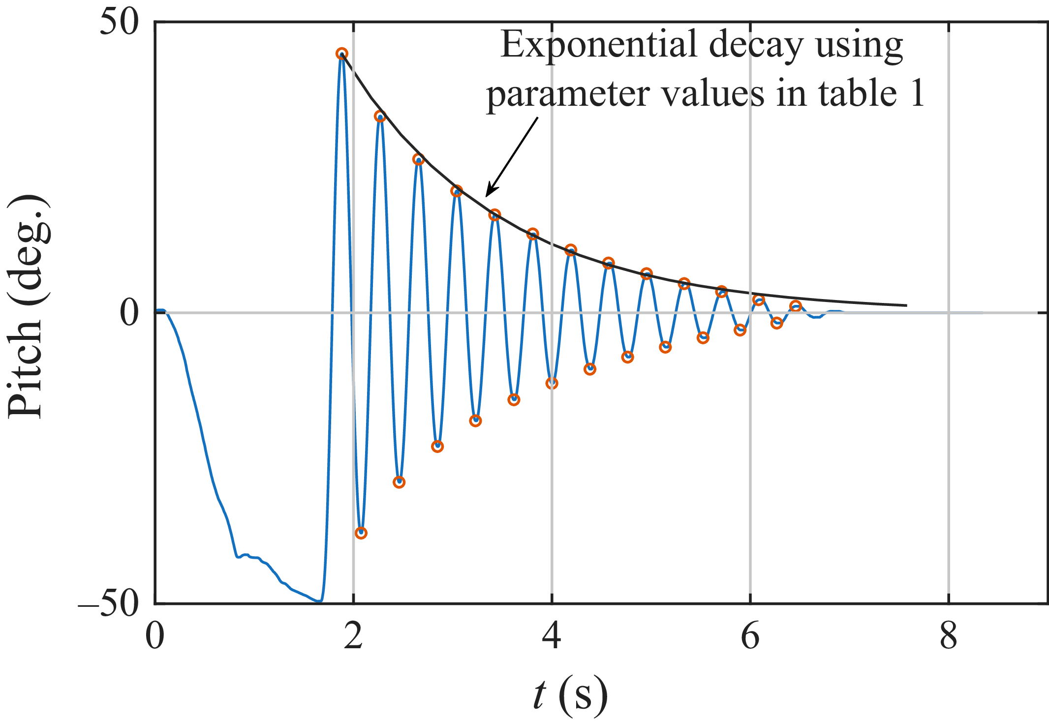

 U∞=10ms−1
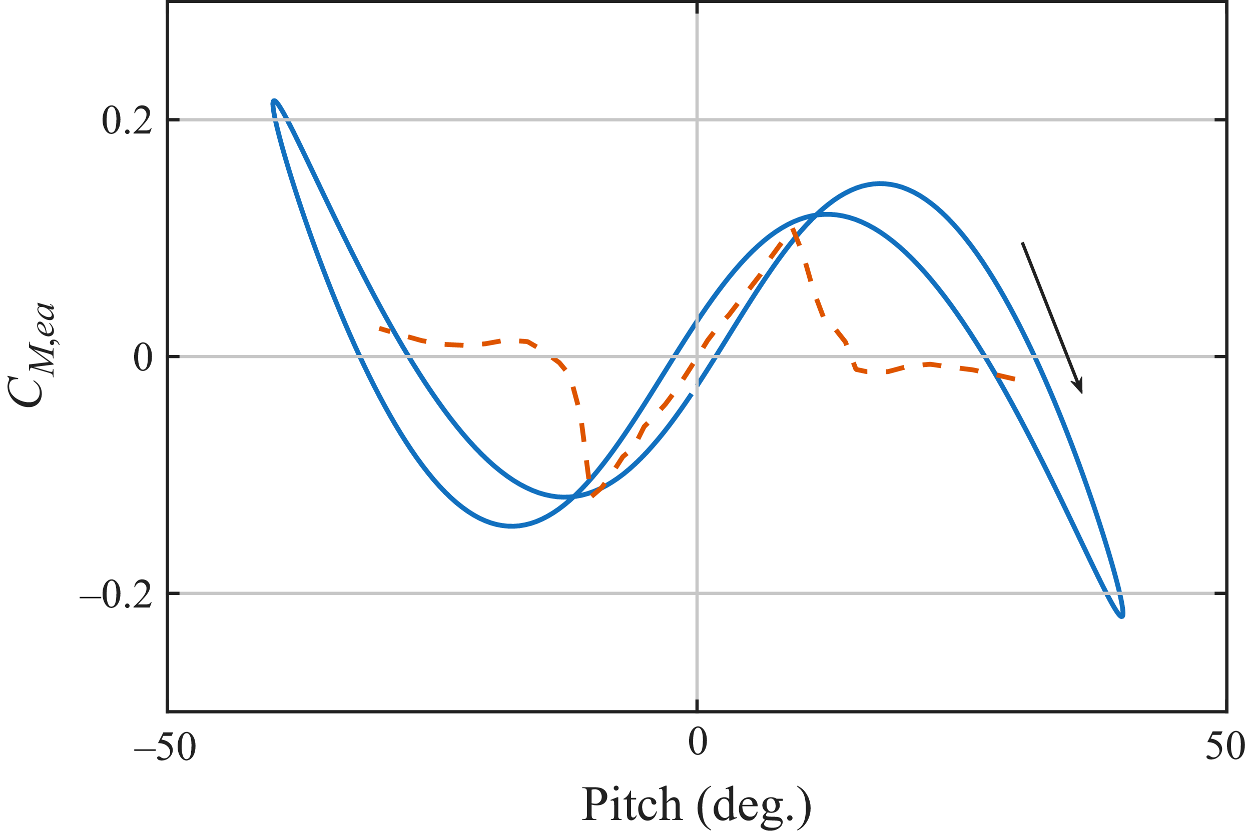
 0.35c
 U∞=10ms−1
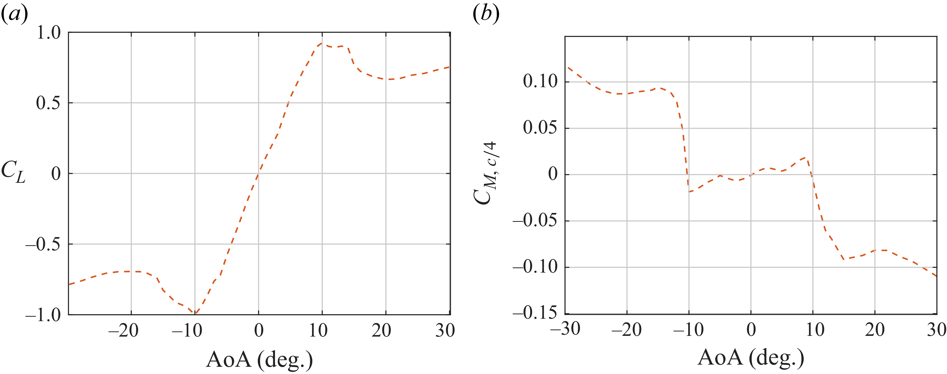
 c/4
 Rec=12×104

 u
 v
 12∘
 U∞=10ms−1

 fg=2.5
 fθ,0=2.93
 U∞=10ms−1

 fg=2.96
 fθ,0=2.93
 U∞=10ms−1

 fg=3.5
 fθ,0=2.93
 U∞=10ms−1

 U∞=10ms−1
 fθ,0=2.93 Hz
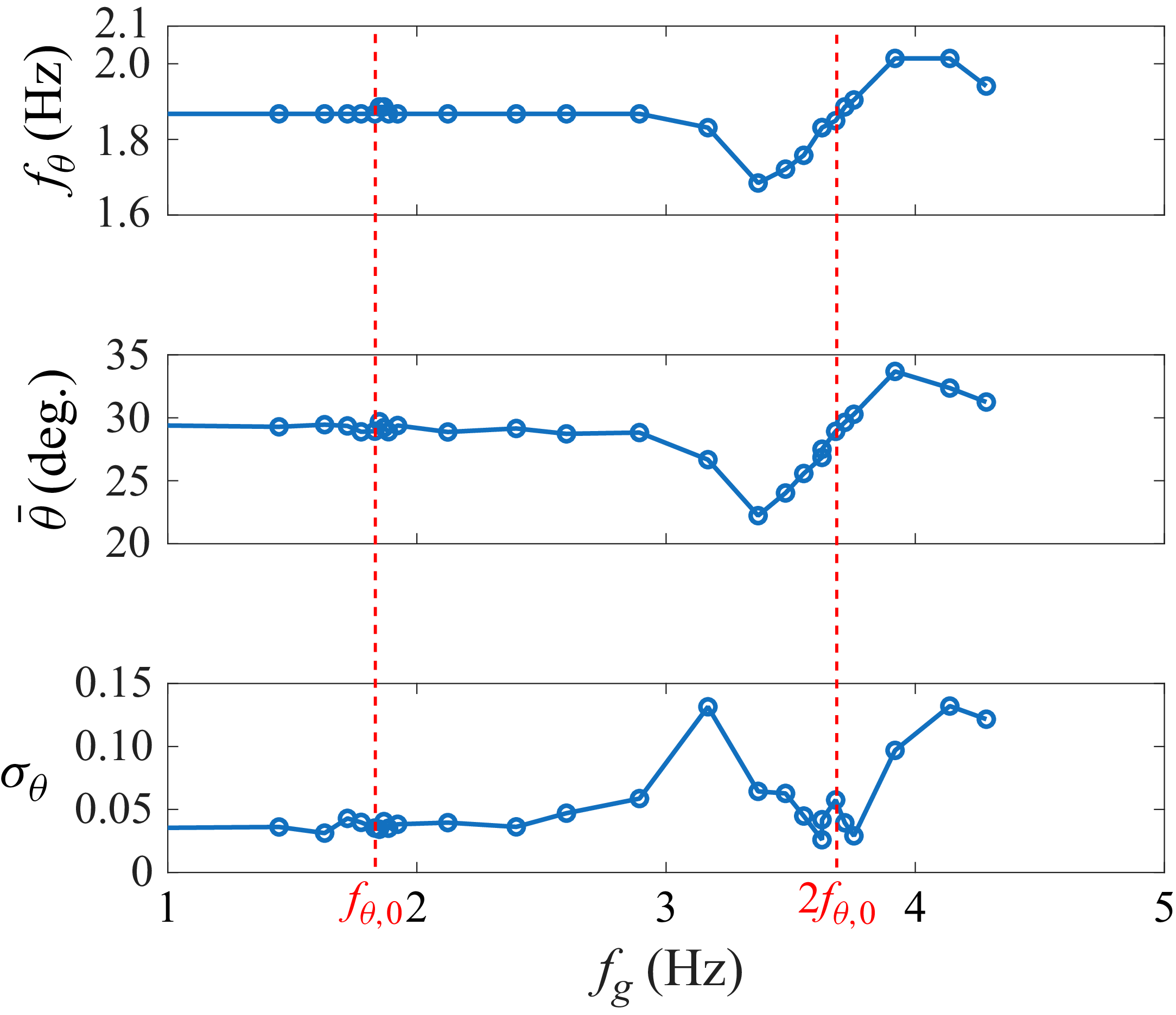
 U∞=7ms−1
 fθ,0=1.87 Hz
 2fθ,0

 fg=3.19
 fθ=1.83
 U∞=7ms−1
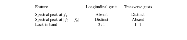

 U∞=7ms−1
 fg=3.19Hz
 fθ=1.87Hz
 fg=3.54Hz
 fθ=1.77Hz

 fi=mfθ+nfg

 fg=2.5Hz
 fθ,0=2.93Hz
 θ¯0=41∘
 ε=0.2

 fθ,0=1.87
 θ¯0=29∘
 ε=0.26

 fθ,0=1.87Hz
 ε=0.2
 θ¯0=19∘,29∘,39∘

 fθ,0=1.87Hz
 θ¯0=29∘
 ε=0.1,0.2,0.3

 fθ,0=1.87Hz
 θ¯0=29∘
 ε=0.05,0.1,0.2,0.4,0.6
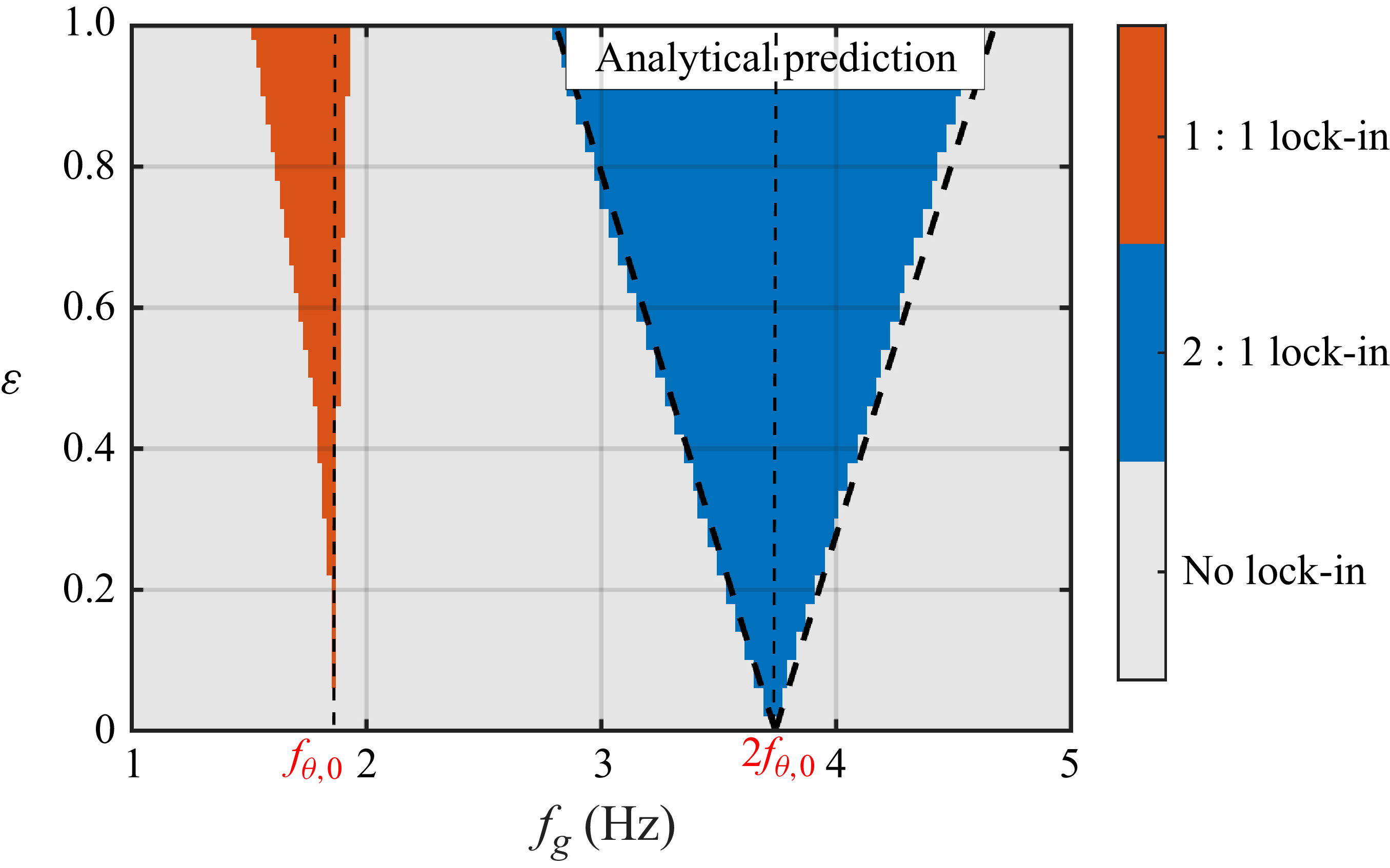
 fθ,0=1.87
 θ¯0=29∘
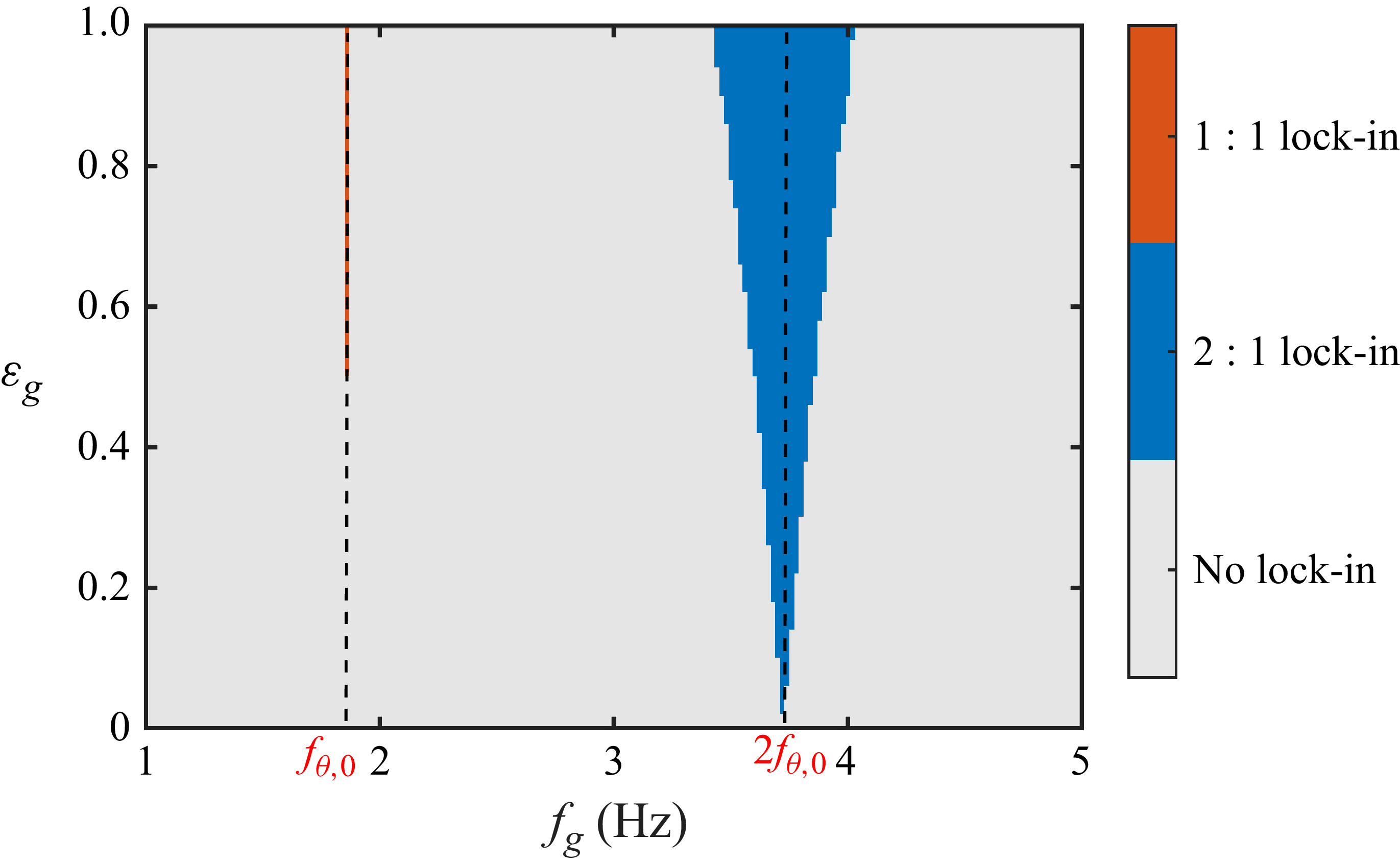
 fθ,0=1.87
 θ¯0=29∘

 fθ,0=1.87Hz
 θ¯0=29∘
 εg=0.1,0.2,0.4,0.8
 θ¯


