1. Introduction
Ice sheets are held in place by friction at their base. The distribution of subglacial water beneath the polar ice sheets controls the flow speed and flow style of the overlying ice. When water is present, friction is reduced and strain rates tend to increase, threatening their seasonal stability. Reference Zwally, Abdalati, Herring, Larson, Saba and SteffenZwally and others (2002) report strong indications that subglacial lubrication has led to accelerated ice flow in Greenland.
To succeed in modeling the behavior of major ice sheets, it is fundamental to find or constrain the extent of any basal melting. There has been progress in Antarctica, but less so in Greenland.
Investigators have used radio-echo sounding (RES) as the primary means of measuring the depth of ice, in the form of ice sheets, ice streams or glaciers (Reference Dowdeswell and EvansDowdeswell and Evans, 2004), for several decades. The radar signal intensity is affected by the presence of subglacial water, which was inferred at Sovietskaya and reported to the International Symposium on Antarctic Glaciological Exploration in 1968 by Reference Robin, Swithinbank and SmithRobin and others (1970). Lakes were identified by Reference Oswald and RobinOswald and Robin (1973) and confirmed by Reference OswaldOswald (1975). Several investigators (e.g. Reference Gades, Raymond, Conway and JacobelGades and others, 2000; Reference Catania, Conway, Gades, Raymond and EngelhardtCatania and others, 2003; Reference Peters, Blankenship and MorsePeters and others, 2005; Reference Siegert, Taylor and PayneSiegert and others, 2005) have used the signal intensity to discriminate between basal water and rock, particularly in Antarctica. Since then these features have been studied extensively in relation to their interconnection, the interchange and flow of water, the potential for the persistence of subglacial life, the inadvisability of dumping nuclear waste, their effect on glacial flow, etc.
For Greenland, radar data have been acquired by the University of Kansas as part of NASA’s Program for Arctic Regional Climate Assessment (PARCA). This dataset is now hosted by the Center for Remote Sensing of Ice Sheets (CReSIS).
The radar data have been used primarily to show the basal topography of the Greenland ice sheet. Echo intensities have been reported by Reference Layberry and BamberLayberry and Bamber (2001) as part of the PARCA program, but, due to a lack of precise calibration and other unknowns, no explicit determination of the extent of basal melting has been made.
The procedure reported here is most appropriate for Greenland radar data. Although water is present, it does not appear to form lakes as found in Antarctica (e.g. Reference Siegert, Taylor and PayneSiegert and others, 2005), where the intensity, continuity and reduced spatial fading of radio echoes reveal smooth topography on a large scale. The procedure is based on the numerical and contextual study of radio echoes, interface geometries, the physics of ice and water and the known glaciological evidence. Statistical analysis of the echo characteristics yields strong evidence that distinct interface types can be characterized from the data. Findings at the GRIP (Greenland Icecore Project) and NorthGRIP core sites provide controls for the validity of the detection of subglacial water (Reference Dahl-Jensen, Gundestrup, Gogineni and MillerDahl-Jensen and others, 2003). Comparison of surface and lower interface gradients, and associations with internal layer disturbances give further support. The trial dataset is based on survey flights (∼4000 km total) undertaken on 14 and 25 May 1999.
This paper outlines the available survey data (section 2), and goes on to describe the method for discriminating, at each point of the radar survey, whether the local substrate interface consists of ice and rock, or whether there is an intervening layer of water (section 3). It then reports findings from the PARCA surveys (sections 4 and 5) that indicate the presence of subglacial water. Section 6 discusses the interface geometry and further validating aspects of the received signals and section 7 provides plots of signals and a map of detected water within these flight segments. Section 8 concludes that the PARCA dataset contains more information than ice depth alone, including the occurrence of basal water.
2. Parca/CReSIS Greenland Remote Sensing
NASA started the research program PARCA in the 1990s with a goal of determining the Greenland ice sheet’s mass balance (Reference Thomas and InvestigatorsThomas and others, 2001). It consisted of coordinated satellite, airborne and in situ observations. The airborne observations consisted of precision surface elevation measurements with a laser altimeter (Reference KrabillKrabill and others, 2002) and ice thickness measurements with a coherent radar depth sounder (Reference GogineniGogineni and others, 2001). The airborne instrument package included global positioning system (GPS) receivers to allow the same flight-lines to be flown a few years apart, in order to determine changes in ice surface elevation and precision geolocation using differential GPS techniques.
The coherent radar depth sounder operates at a center frequency of 150 MHz. The transmitter generates a pulse of 1.6 μs duration and 200 W peak power (actual transmit power is ∼70 W because of cable losses), which is frequency-modulated over a bandwidth of 17 MHz. It uses two antennas that are mounted under the left and right wings of the aircraft: one for transmission and the other for reception. Each antenna is a four-element dipole array with two-way beamwidths of 18° and 66° in planes perpendicular and parallel to the flight path, respectively. The receiver amplifies and compresses the received signals in a weighted surface acoustic wave (SAW) compressor to an effective pulse duration of ∼60 ns. This results in a depth resolution of ∼5 m in ice. The compressed signal is coherently detected and integrated by summing consecutive pulses. The coherent integration serves as a low-pass filter and reduces the effective along-track beamwidth. In this case, integration over ∼3.6 m of track (pulse repetition frequency (PRF) 9.2 kHz, aircraft speed 130 m s−1, N (coherent integration) = 256) reduces the beamwidth in ice from 66° to ∼17°.
The airborne system was used to collect an extensive dataset of ice-elevation and ice-thickness measurements over much of the ice sheet during 1993–2006, and these data were distributed rapidly to the community through the World Wide Web. Prior to 1997, we used a digital system with 8-bit analog/digital (A/D) converters that was only capable of storing incoherent or coherent data with a large number of pre-summed signals (in order to reduce data volume) at a low PRF of 2000 Hz. We incrementally upgraded the radar depth sounder to improve performance and save coherent data to synthesize a large aperture in the along-track direction. We developed an improved coherent radar with a new digital system incorporating 12-bit A/D converters and field-programmable gate arrays (FPGAs) to digitize and store the in-phase and quadrature signals with as few as 32 pre-summed returns for 1024 range cells at a PRF of 9200 Hz. The new digital system also performs preliminary processing and displays processed data in real time for the operator. We started using the improved radar depth sounder routinely during the 1998 field season. The amplitude and phase information are saved for data collected during and after the 1999 field season. Table 1 lists the important system parameters.
System parameters

We have estimated the uncertainty in radar ice-thickness measurements to be within ±10 m based on comparisons with ice-core locations at both high-elevation interior sites and an outlet glacier (Reference GogineniGogineni and others, 2001).
PARCA survey flights sampled much of the area of Greenland, and have been described in Reference GogineniGogineni and others (2001). The subset used in this analysis is shown in Figure 18.
An example of an ice radar profile is shown in Figure 1. This represents a 150 km segment of a PARCA flight on 14 May 1999. Ice depth is measured down from the upper horizontal green line, and the base of the ice is represented by the trace near 3250 m depth. Flight data have been processed in 33 km subsegments, forming extended flight segments of several hundred kilometers.
Example of a radar ice profile. The upper green horizon represents the ice surface. The lower irregular horizon near 3250 m on the vertical axis represents the bed of the ice, and intermediate layers reflect the internal layer structure of the ice.

3. Theory and Method
3.1. Background
Signals received by a radar sensor are typically estimated by means of the well-known radar range equation (e.g. Reference SkolnikSkolnik, 1990). In the case of radio-echo sounding this equation needs to be modified to allow for the effects of reflection and scattering from the extended, rough interface rather than from a point target, and for the effects of propagation through the solid medium and its air interface. Propagation losses in the dielectric medium are generally represented by an exponential decay factor.
Basic theory of the scattering of an electromagnetic wave by a rough interface, as between ice and subglacial rock, has been given by Reference Beckmann and SpizzichinoBeckmann and Spizzichino (1963) and by Reference BerryBerry (1973), and is based on Kirchhoff diffraction theory. Explicit solutions have been based on constrained statistical parameters (Gaussian, isotropic and randomly distributed vertical roughness scales and horizontal correlation lengths) and derived quantities (first return, scattering loss and fading length). These quantities introduce added uncertainties in the radar equation.
Berry has provided a rigorous analysis of the effects on echo first-return amplitude and tail extent for certain statistically stationary and isotropic rough interfaces, defined in terms of vertical root-mean-square (rms) displacement and horizontal autocorrelation properties. This powerful demonstration shows that these interface characteristics, as defined, are difficult to infer from the chosen signal attributes except in certain extreme cases.
Recent practice is described by Reference Gades, Raymond, Conway and JacobelGades and others (2000), who calculate intensities for a wideband high-frequency radar (3–4 MHz) for which the radar wavelength of ∼50–70 m in ice is large compared with much small-scale roughness on the interface. However, Gades’ window definition is not applicable to the University of Kansas pulsed 150 MHz radar. Relevant work on large-scale interface roughness is also described by Reference Siegert, Taylor, Payne and HubbardSiegert and others (2004).
Fountain (e.g. Reference Fountain, Jacobel, Schlichting and JanssonFountain and others, 2005) describes water inclusions within temperate glaciers, and Reference Peters, Blankenship and MorsePeters and others (2005) describe a relevant method based on absolute reflection coefficients and used in Antarctica with radar calibrated against a planar sea-water target. Their paper gives a comprehensive summary of the method and its history, and may be taken as state-of-the-art with respect to the standard analysis for a calibrated radar.
3.2. An energy-focused, statistically robust method
Neither scattering losses nor fading describe processes in which energy is actually lost. These factors result from the divergence of energy away from the nominal specular reflection path and the resulting interference effects. The first return is only one component of the received signal, and by aggregating the whole echo envelope, incoherently averaged over fading, we recover the divergent energy, whose total is more directly related to the basal material properties. Appropriate measures are summarized in Table 2.
Input and output variables

The description used for the scattering interface is not confined to particular roughness statistics. Neither a singular scale of roughness, nor an assumption of isotropy is imposed. Instead of prescribing stationary statistical parameters such as the rms vertical deviation of the interface (which presupposes a level mean surface), we constrain broadly the angular distribution of its slopes, and the effect of curvature of the interface in terms of diffraction.
The distinction between reflection and scattering or diffraction is not important, since both are mechanisms whereby the returned energy is redistributed, not lost. We evaluate whether the total divergence is greater than the effective beamwidth: provided that the returned energy is captured and averaged over fading, power variance should be reduced.
By contrast, dielectric absorption reduces the propagating energy in the fabric of the ice and must be accounted for. Our only assumption has been that the absorption rate does not vary rapidly with position on the scale of the thickness of the ice or less, and that it therefore does not account for rapid changes seen in basal reflection intensity.
The results bear this out. Consistent relative intensities have been obtained using a simple formula for the rate of absorption in ice with depth, varying with the surface elevation as a proxy for ice temperature. This has been applied over the whole trial dataset without introducing unexpected variations. This theory has been tested by observation of the resulting intensity statistics and demonstrated by the narrow distributions that result.
Using the statistics afforded by the broad coverage of each flight, a lower reference point has been fixed for each extended flight segment, representing the reflecting power of an interface between ice and rock of medium permittivity. This has then allowed recalibration of the radar, based on observed intensities for rock.
Reflection coefficients can then be discriminated. We obtain validation of the presence of water through analysis of basal and surface slopes and by association with coring results and other glaciological features. Table 3 illustrates the result of the process.
Outline of analytical results

3.3. Intensity spread vs the range of reflection coefficients
If peak signal intensities are only corrected for geometrical effects, the received intensity is found to vary over a range of ∼40 dB or more, which has proved too great to detect the effect of variation of the basal reflection coefficient reliably. Three example intensity distributions are illustrated in Figure 2. Figure 3 illustrates the expected reflection coefficients between ice and rock or water–till mixes of various permittivities. Rock varies in permittivity between ∼4 and 12, and a water–till mix can vary from ∼10 to 80. There is little overlap, but we may expect that reflections from frozen and melting substrates will differ by ∼10 to 15 dB, or less, as the fluid incorporates increasing proportions of till. This is much less than the observed spread of intensity. To discriminate water infiltration reliably, the intensity spread must be narrowed.
Example intensity distributions. After correction for geometric divergence, the received intensity varies over a range of >40 dB.

Reflection coefficient vs relative permittivity. The range, between −3 and ∼−15 dB, is much less than the geometrically corrected intensity variation.

3.4. Intensity corrections for propagation effects
3.4.1. Interference
Interference plays a dominant role in determining the reflected signal at any particular position. However, interference does not affect the distribution of the signal intensity once this is averaged incoherently over a certain minimum distance, provided that the fading length is more than twice the coherent integration distance used prior to recording. The received power is a function, P r(D, x), of depth D and distance along track, x.
Observed fading interval. For the trial dataset the fading of the peak basal return tends to occur over distances between 15 and 100 m. For a depth of 3000 m, this suggests that fading results from interference between principal facets separated by 20–120 m. This is shown in section 3.4.2 to be within the illuminated area of the radar, of radius 112 m, diameter 224 m.
In 1999, coherent integration was applied over a distance of ∼4 m, and reflections and fading from more widely separated facets than ±8° were reduced.
Incoherent averaging. By averaging received intensity incoherently over a flight distance of 200 m, variations due to the observed interference are smoothed. Successive values refer to separately illuminated reflecting surfaces that are likely to be uncorrelated. The signal intensity variance is reduced.
3.4.2. Reflection divergence
Observation of the echo envelope shows whether the observed reflections are limited by the beamwidth of the antenna. Provided that this is not the case, although the beam is broadened either by rough-surface reflection or diffraction, the higher-angle facet reflections or diffraction fringes will still be received, albeit with a greater delay. On average, for a continuous but irregular interface, as much energy is scattered into the beam as is lost, albeit from an increased slant range. Returns at higher angles contribute to an extension of the pulse envelope. Figure 4 illustrates the extension of the pulse envelope due to divergence of the reflected wave for (a) smooth, (b) slightly rough (∼0–5° slopes) and (c) rough interfaces. If diffraction can be neglected, the envelope will be directly related to the angular distribution of the interface.
The echo is extended due to divergence of the reflected wave and reflection from facets at increasing radii around the nadir point. Pulse envelopes are shown for (a) smooth, (b) typical, slightly rough (∼0–5°) slopes and (c) rough interfaces (at the scale of the pulse length).

Siegert (e.g. Reference Siegert, Taylor, Payne and HubbardSiegert and others, 2004) has worked extensively on interface roughness at the scale of the macroscopic roughness of the depth measurement, with variance of tens or hundreds of meters and length scales >5 km. This is distinct from roughness on the scale of meters or less that determines the reflecting or diffracting characteristics of the interface.
Returns from interfaces that are smooth at this scale (the pulse-length scale) will be representative of the substrate characteristics in reflecting power and angular distribution.
Primary illuminated area. The area illuminated by the radar pulse and contributing to the primary reflection is calculated. For an interface that is flat at the scale of the ice depth, the area illuminated by the pulse such that it extends the initial echo return by <50% has a radius of approximately  , where D is the depth, p is the radar pulse half-width in air and ε
ice is the relative permittivity of ice (3.2). For R = 3000 m and p = 7.5 m, then R
p = 112 m. This may be taken as a definition of the ‘first return’.
Divergence and beamwidth. The antenna beam is described by Reference Legarsky, Chuah and GogineniLegarsky and others (1997). The across-track beam pattern is approximated by the red line in Figure 5, in which the blue curve illustrates the angular spectrum of a typical received signal, estimated from the envelope broadening using the assumption of a coarsely flat interface and plotted against off-nadir angle.
Received power and beam vs across-track angle. This illustrates that in a typical case the angular distribution of returns is narrower than the beam pattern, and that most reflected energy is included within the beam.

The received energy lies within the antenna across-track beamwidth, but may exceed the beamwidth along track due to coherent integration. This may affect the aggregate received power, and would have the effect of extending the distribution of intensity at its lower edge.
To ensure the selection of interfaces that are sufficiently smooth at this scale, so that reflected and scattered energy are collected efficiently, a threshold is imposed on the abruptness of the signal in selecting returns as representative of increased dielectric contrast at the interface.
Aggregation of pulse energy. Echoes over the whole basal reflection envelope, representing returns from all directions within the beam pattern, are then aggregated. This further reduces the variance of the received signal.
Reflection abruptness. The abruptness index of the received signal is defined as:

where the numerator is the peak basal reflection intensity received at a position x along the flight path, the denominator is the aggregate basal reflection intensity and D int is the interval of depth bins included within the aggregate. The value of I abr normally lies between 0.05 and 0.5, which is the maximum for this pulse length and sample rate. Typical values indicate a primary illuminated area of radius less than 300 m at depths of 2000–3000 m, and frequently less than 180 m. Such radii show that some energy is lost from the ‘first return’, but also that the reflections are contained within a relatively narrow range of angles from the nadir.
Whether resulting from reflective or diffractive processes, I abr places a constraint on the angular spectrum of the received signal. If this exceeds the effective beamwidth of the receiving antenna, there will be additional losses. In typical cases, the shape of the received waveform envelope limits the angles of arrival of basal signals, at levels less than −10 dB or more below the peak, within about 18° of the vertical either along or across track. This is illustrated in Figure 5.
3.4.3. Dielectric losses
The intensity reduces with depth as a function of the geometric wavefront spreading, based on an inverse-square law. However, there are also losses, exp(−BD), where B is the attenuation rate, due to propagation through the solid ice which, as a dielectric, has a finite loss tangent and causes attenuation. Losses with depth varying from B = 1.4 ± ∼0.1 dB (100 m)−1 for a surface altitude H = 3000 m, to 2.3 ± ∼0.1 dB (100 m)−1 for a surface at 1000 m account for the observed intensity variations as a function of depth, using the formula:

The mean, aggregate and depth-adjusted received signal intensity still retains variability due to the large-scale curvature of the interface which, subject to slope limits related to the beamwidth, will affect the variance of the signal but not its mean value. The intensity is otherwise representative of the basal reflection coefficient plus any uncalibrated variations in the system.
3.4.4. Recalibration
The PARCA data were acquired with variable receiver attenuation whose setting was not recorded automatically. This may be recovered provided that changes were not frequent.
Common lower limit of reflecting power. After averaging and aggregating the reflected energy, correcting for propagation losses, and given a sufficient measurement population, we typically find a clear lower boundary of the distribution. We interpret this as the effect of typical dry rock interfaces. Most flights exit and return over a common path including a relatively smooth, frozen interface. The lower intensity bound is then used as a reference. The upper bound represents returns from wet interfaces with variable water fractions; as not all flights can be assumed to encounter ‘electrically deep’ water it is less reliable as a reference.
The lower intensity bounds for each extended flight segment are then aligned, yielding distributions that should, if the adjustments are correct, be independent of settings of the radar and sensitive to local variations in the received intensity. A recalibration factor, f cal, with values between 6 and −2 dB, has been added based on the observed lower-bound intensities.
3.5. Adjusted intensities
Taking these various corrections and adjustments into account, the signal intensity is recalculated for all flight positions in the test dataset.
Note that these intensity values are calculated relative to an implicit reference determined by the transmitted power, the antenna gain, its effective area, the absolute reflecting power of the interface and the standard geometric factors. The basic equations and definitions are provided in the Appendix.
4. Observed Intensity Statistics
When these corrections and adjustments are included, the intensity distribution is substantially narrowed for data observed during these flights, by comparison with Figure 3. For reference, the distribution for the flight segment including the GRIP and NorthGRIP drill sites is shown in Figure 6. We note that, after adjustment, the lower (rising) edge of the distribution occurs over an interval of 4 dB, with little evidence of extension due to loss of signal within the integrated beam pattern. The distribution has an effective base width a little over 20 dB, as opposed to the >40 dB width of the unadjusted distribution. It also appears to contain two populations with different mean values of intensity. It is plotted with the sum (in red) of two Gaussian curves separated in mean value by 10 dB. Of this population 63% is derived from the lower fraction and 37% from the higher. This curve is used later as a reference. Different subsets of this flight segment exhibit clearly different characteristics. Taking subsegments 46–48 and 52–54 (each 99 km long), the sub-distributions are shown in Figure 7.
Intensity distribution for 14 May 1999, segment 45–54. After adjustment of intensity for interference, absorption and divergence, this gives a clear illustration of a bimodal population (cf. Fig. 2). The flight length is ∼330 km, containing over 1500 independent intensity samples. The red curve illustrates hypothetical Gaussian distributions separated by 10 dB.

Intensity distribution for 14 May 1999, subsegments 46–48 (red; frozen) and 52–54 (blue; wet). These separate 99 km subsegments yield narrow and easily discriminated intensity distributions.

These distributions contain large populations of independent values (1500 for Fig. 6 and 450 for each curve in Fig. 7) and are distinguishable at a very high level of significance, with a mean separation close to 13 dB and standard deviation of ∼4 dB. As the ability to distinguish between these distributions is somewhat contentious we provide further examples below.
4.1. Statistical confidence
To confirm the statistical significance of the differences in these populations, a Student’s t test has been applied. To summarize, the derived value for t of ∼30 for the ‘high’ and ‘low’ populations (each of which represents a 99 km subsegment) suggests that they are statistically distinguishable at a confidence level better than 1 – 10−6.
The signal intensities cannot be part of the same population, and represent very different interfaces in this respect. Subsegment (ss) 46–48 coincides with the site of the GRIP borehole (at ss 47.9), where the bedrock was found to be frozen. Subsegment 52–54 coincides with the site of the NorthGRIP borehole (at ss 54.3), where the drill encountered water, confirming this assignment. Further means of verification are described in section 6 below.
4.2. Reflection intensity distributions for test segments
To illustrate the method in greater detail, we use segments from 14 and 25 May 1999 with these adjustments, shown in Figures 8–12. Each flight contains subsegments that contain either predominantly high-reflectance or predominantly low-reflectance interfaces, corresponding well with the (ice–water) or (ice–rock) expectations. These can be seen as prototypes of frozen and melting interfaces. The subsegments used are 33 km long, yielding populations of about 150 independent values each and yielding similarly significant t values.
14 May 1999: (a) segment 13–27, including frozen and wet basal materials, (b) subsegment 14 (frozen) and (c) subsegment 18 (wet). The red curve illustrates hypothetical Gaussian distributions, derived from Figure 6 and normalized.

14 May 1999: (a) segment 42–70, including frozen and wet basal materials, (b) subsegment 47 (frozen) and (c) subsegment 54 (wet). The red curve illustrates hypothetical Gaussian distributions, derived from Figure 6 and normalized.

25 May 1999: (a) segment 21–38, including frozen and wet basal materials, (b) subsegment 25 (frozen) and (c) subsegment 34 (wet). The red curve illustrates hypothetical Gaussian distributions, derived from Figure 6 and normalized.

25 May 1999: (a) segment 40–46, including frozen and wet basal materials, (b) subsegment 42 (frozen) and (c) subsegment 43 (mixed frozen and wet). The red curve illustrates hypothetical Gaussian distributions, derived from Figure 6 and normalized.

25 May 1999: (a) segment 65–85, including frozen and wet basal materials, (b) subsegment 78 (frozen) and (c) subsegment 74 (mostly wet). The red curve illustrates hypothetical Gaussian distributions, derived from Figure 6 and normalized.

Subsegments 14 and 47 appear to be dominated by frozen bedrock (verified by GRIP), while subsegments 18 and 54 are dominated by water (verified by NorthGRIP).
Flight segments from 25 May yield similar components. Subsegments 25, 42 and 78 appear to be dominated by frozen bedrock, while subsegments 34 and 74 are dominated by water. Subsegment 43 contains a separable combination of frozen and wet bases similar to that in Figure 6, but with a smaller population.
These intensity statistics indicate that water is present over extended but finite distances within each of these flight segments. It does not form continuous lakes as seen in Antarctica (the intensity still varies sharply within each subsegment). In these results for Greenland, the water appears to form a continuing, but punctuated, layer.
Following this determination, further descriptive and validating information about the subglacial interface is provided in the following sections.
5. Validation by Association
Many instances where water is detected by this method are also associated with disturbances in the internal layer features in the ice. Figure 13 illustrates a section of ice profile in which water is detected twice at the base. This coincides with distortions of the corresponding internal layer structure, giving evidence for lost and stressed ice. Such associations are frequently found with identified basal water. Without a change in the basal material, disturbance of the ice would be expected to diffuse transmission rather than to focus the wave, causing a reduction rather than an increase in intensity. Quantitative study of internal layer disturbance would be rewarding, following Reference Fahnestock, Abdalati, Joughin, Brozena and GogineniFahnestock and others (2001).
14 May 1999, segment 60–63. Water is detected at the base within the dotted outlines. Layers in the overlying ice are distorted. The locations are determined from the coherence index and a threshold. Coherence is calculated from the complex received signal, independent of the intensity, and the abruptness index, and is related to smoothness at the wavelength scale.

6. Interface Geometry of Subglacial Ponds
A discussion of reflection intensity and basal materials is incomplete without considering the geometry of the interface and the infiltrating water.
Water is formed under pressure when ice is near its melting point. It is denser than ice and will gather at low points in the rock unless forced out by a pressure gradient. Shear stresses are eliminated by a water layer whose upper surface will tend to flatten if the ice pressure varies slowly over the scale of the local roughness. Near the pressure-melting point, excess contact pressure will also be relaxed by melting.
The lower surface of an included water body will be determined by the rough shape of the underlying rock. The ice–water interface will therefore tend to be smoother than nearby ice–rock interfaces. However, this relaxed state can change dramatically under conditions where melting and regelation lead to crack growth and fracture.
The radar signals provide an indication of the smoothness of the interface at three levels, described in the following three subsections.
6.1. Large-scale interface smoothness
The radar signal provides a measure of the smoothness of the basal interface on scales greater than the pulse length, measured by the delay of the pulse as a function of distance along the profile. Figure 1 illustrates a bed with relief of ∼140 m with some smoother sections, while Figure 14 illustrates steep relief, also with smoother sections.
25 May 1999: (a) a region of steep relief in the basal topography, over a depth of ∼3000 m; (b) the adjusted echo intensity; (c) the echo abruptness; and (d) the coherence index. Arrows in (a) indicate where the coherence index exceeds 0.3.

6.2. Interface smoothness at the pulse-length scale
Section 2.4.2 described the relationship between slopes in the rough reflecting interface and the extension of the received pulse envelope. Considering that such reflections arise from interface facets of about the size of a first Fresnel zone (∼80 m), the vertical roughness at this scale can be constrained on the basis of the abruptness index (defined in Equation (1)). For facets with up to 5° gradients, we infer vertical roughness of up to at least a few meters within the primary illuminated area.
The abruptness index varies from <0.05 to the expected maximum of 0.5. Although high values of the abruptness index are clearly correlated with high aggregate intensity, abruptness is not used as a proxy for intensity because rock intensity levels are also found with relatively abrupt reflections. Specific identifications of water bodies will be restricted to those where the reflection is both intense and abrupt, to avoid spurious effects of curvature or diffraction. To identify locations that are significantly smooth at this scale, a threshold at half the maximum index value, or 0.25, is used.
6.3. Interface smoothness at the wavelength scale
A third measure of smoothness is available at the yet smaller scale of the wavelength. This is the coherence index, I co, which is related to the radio wavelength and is defined as:

where D is the echo depth, x is the distance along track, X int is the along-track distance interval for both coherent and incoherent integration, and D int is the aggregation interval including the basal echo envelope. The integral in the numerator sums the complex echo signal, ψ, over X int, and is evaluated for a slope, θ g, which maximizes the coherent integral. The denominator is the integral of signal power over the distance and depth intervals. This equals the coherent integral at θ g for a flat interface, where I co = 1.
Over increasing integration distances the coherent integral will tend to zero. However, if surfaces that are flat (in terms of the wavelength) persist over distances comparable with or greater than the first Fresnel zone diameter (∼80 m), then coherent returns will be visible, a smooth interface is inferred, and its slope can be derived.
Here we have performed the integrations over ∼200 m, and values of I co > 0.3 indicate surface facets that are flat to within ∼0.2 m over that distance. Within the deep relief there are significant flat areas, although none qualifies as a ‘lake’.
Figure 14 illustrates deep interface relief in central Greenland with the aggregate intensity, corrected for depth and absorption (Fig. 14b), the reflection abruptness, related to smoothness at the pulse-length scale (Fig. 14c), and the reflection coherence, related to smoothness at the wavelength scale (Fig. 14d). Arrows in Figure 14a indicate locations where the coherence index exceeds 0.3, indicating substantially flat interface facets.
A subglacial water interface may be in equilibrium with the ice above it, without disturbance by internal stresses. If so, the interface will tend to be smoothed and its slope will take a value so that the pressure gradients are balanced beneath the ice overburden. The water surface slope will be related to the ice surface slope by a factor of −ρ i/(ρ w − ρ i), where ρ i is the density of ice and ρ w is the density of water. The expected value for the slope ratio is −11.5.
Taking the locations where the coherence index exceeds a threshold of 0.3, the basal slopes are determined and plotted against the corresponding surface slopes obtained from a digital elevation model. Figure 15 shows the result. The points are scattered around a regression line giving a gradient of −12, which suggests a fluid density of 0.99. This is significant. It provides a direct link with the physical characteristics of water, giving an opportunity for validation of the presence of water without the need to drill through the ice. It therefore reduces reliance on the three drilled reference points.
Interface slopes and surface slopes for the arrowed locations in Figure 14a. The regression gradient of −12 would correspond to an equilibrium fluid density of 0.99. This value directly links the smooth facets with the physical characteristics of water.

Figures 16 and 17 contain the profiles of the segments described above, together with signal intensity (magenta traces), abruptness (dark blue traces) and coherence (light blue traces). Superimposed are the positions of water inclusions as determined by the combination of high intensity and high abruptness (blue diamonds).
14 May 1999: segment 42–70 (which includes North GRIP at location N in Fig. 18). The surface profile, bed profile, depth-adjusted intensity, echo abruptness and echo coherence are plotted.

25 May 1999: segment 40–46 (which includes location M in Fig. 18). The surface profile, bed profile, depth-adjusted intensity, echo abruptness and echo coherence are plotted.

7. Example Profiles and Plotted Results
Figures 16 and 17 contain profiles of depth, signal characteristics and locations of subglacial water for all the flights studied.
Although the traces appear ‘noisy’, and filtering might be recommended, this is the result of the high degree of horizontal compression of the figures, each representing several hundred kilometers of flight. Each point should be considered as representative of the local characteristics of the bed; low-pass filtering will introduce unrealistic smoothness and unrepresentative intensity, abruptness or coherence values.
The horizontal compression also leads to overemphasis of basal water due to the thickness of the printed traces. In particular, the abruptness curve gives the impression that the threshold is exceeded continuously, whereas in fact the trace consists of frequent, but discontinuous, excursions over the threshold.
The traces contain information on which we base our decisions as to the presence of water. Where in a locality the intensity remains at a high level but the abruptness falls, disqualifying the point as water, this may be due to a rough, non-equilibrium interface. In these cases, there may be some underestimate of the extent of water. Coincident determinations arising from cross-points between flights have not yet been evaluated exhaustively, but can be seen generally to confirm the presence or absence of sub-glacial water.
Cases also exist where, although the surface is smooth and the intensity context is high, the local intensity level falls. In some cases, this coincides with aircraft turns and is believed to be due to the effect of the aircraft’s bank and the antenna beam pattern.
These results indicate that the PARCA radar data can be used to recover information about the extent of water infiltration that agrees with all available sources of validation. It also shows a substantial incidence of subglacial water, with high spatial precision, that demands further attention and inclusion in Greenland ice-sheet models.
Figure 18 maps these flights and the results in terms of the extent of subglacial water.
The distribution of subglacial water determined from echo intensity and abruptness for the trial dataset. Frozen bed is indicated by green diamonds, and water is represented by blue diamonds. Approximately 17% of the flight length is determined as wet. Some regions are wet for more than 80% of flight distances of >100 km.

8. Conclusions
These flight segments yield plots of the distribution of water (blue) and frozen (green) interfaces, shown in Figure 18, indicating the presence of basal water over at least 17% of the flight distance covered.
In certain areas the proportion is over 80% for distances of >100 km. This indicates that large ice volumes in Greenland have lubricated basal interfaces.
These results, combined with the sources of validation described above, provide a strong body of evidence that the presence and extent of subglacial water can be recovered from the data provided by the PARCA program. We plan to extend this analysis over as much of the PARCA dataset as possible, and to provide the results to the ice-sheet modeling community, especially within the CReSIS program.
Acknowledgements
We gratefully acknowledge support provided for this work in the form of data provision by PARCA/University of Kansas, the support and expertise of staff at CReSIS, the University of Kansas, and encouragement and facilities provided by staff at the University of Maine Climate Change Institute.
We are also grateful for the comments and advice of reviewers and the scientific editor, which have contributed much to the final form of the paper.
Appendix Equations and Definitions
Variables and equations relevant to the discussion are described below.
-
1. Radar range equation:

where P r is received power, P t is transmitted power, G t and G r are gain on transmission and reception, respectively, λ is signal wavelength, σ is scattering cross-section of the target and R is the range to the radar target. In this case we will replace R with D, the depth to the basal interface.
-
2. Incoherent averaging:
where P is signal intenstity and X int is the flight distance over which averaging is carried out.
-
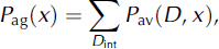
3. Signal energy aggregation:
where P av is the power at a particular depth (D), after averaging over fading. The sum is taken over the range D int from D min to D max, the upper and lower limits of aggregation around the peak basal return; thus D max > D base > D min. P peak is the peak power and D base = D(P peak) is taken to represent the ice depth.
-
4. Adjusted intensity:
10 log [P adj(x)] = 10 log [P ag(x)D 2] + B(D/100) + ρ cal, where P adj is the adjusted, aggregate intensity.