

The argument that two lithic technological traditions existed in western North America during the late Pleistocene is based on evidence that unfluted, stemmed-haft projectile points occur in archaeological contexts that are the same age as Clovis components from sites in the Great Plains and Southwest (Beck and Jones Reference Beck and George2010; Davis et al. Reference Davis, Willis, Macfarlan and Rhode2012, Reference Davis, Bean, Nyers and Brauner2015; Jenkins et al. Reference Jenkins, Davis, Stafford, Campos, Hockett, Jones, Cummings, Yost, Connolly, Yohe II, Gibbons, Raghavan, Rasmussen, Paijmans, Hofreiter, Kemp, Barta, Monroe, Gilbert and Willerslev2012). These stemmed projectile points are the hallmark of the Western Stemmed Tradition (WST) or Paleoarchaic Tradition (e.g., Beck and Jones Reference Beck and George1997, Reference Beck, George, Graf and Schmitt2007, Reference Beck, George, Beck and Jones2009, Reference Beck and George2010; Bryan Reference Bryan, Harten, Warren and Tuohy1980, Reference Bryan, Judith, Willig, Aikens and Fagan1988; Davis et al. Reference Davis, Willis, Macfarlan and Rhode2012; cf. Jennings Reference Jennings1957, Reference Jennings, Jennings and Norbeck1964; Willig Reference Willig, Willig, Aikens and Fagan1988). WST artifacts are common west of the Rocky Mountains and, as Davis et al. (Reference Davis, Willis, Macfarlan and Rhode2012) argue, are part of a lithic technological tradition that differs significantly from the Clovis Tradition and its nonfluted technological descendants. WST projectile points tend to be made from a more diverse range of toolstone types and use local sources of varying quality. They are also produced through core technologies that produce flat, linear flake blanks as the primary basis for tool production. However, WST technologies also use a range of core types, including centripetal, unidirectional, and multidirectional forms. Finally, WST assemblages contain evidence that projectile point manufacture was sometimes performed mainly via the pressure flaking of macroblades and macroflakes in contrast to early Paleoindian projectile point forms that were made through more extensive bifacial reduction sequences.
Archaeologists have not studied WST lithic technology to the same degree as its fluted and unfluted Paleoindian counterparts (e.g., Bradley et al. Reference Bradley, Collins and Hemmings2010; Buchanan and Collard Reference Buchanan and Collard2007; Collins Reference Collins2010; Eren and Andrews Reference Eren and Andrews2013; Frison Reference Frison1989; Huckell and Kilby Reference Huckell and David Kilby2014; Kilby and Huckell Reference Kilby, Huckell, Graf, Ketron and Waters2013; Smallwood Reference Smallwood2012; Smallwood and Jennings Reference Smallwood and Jennings2014). As a result, we are less certain how WST lithic tool production varied across time and space. However, excavations at the Cooper's Ferry site in western Idaho have revealed a stratified series of assemblages spanning the late Pleistocene to early Holocene, which offer a unique opportunity to study WST lithic technology.
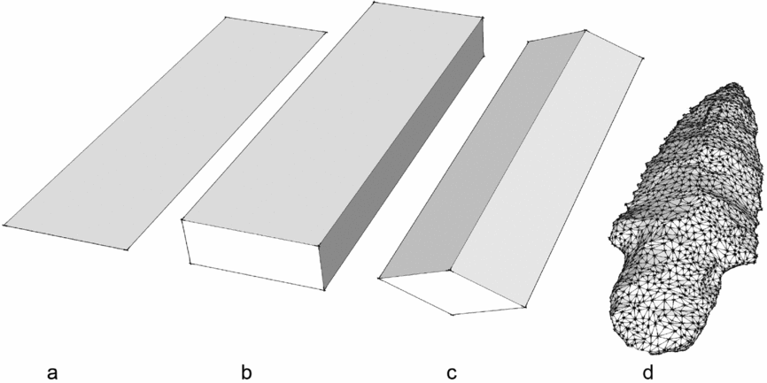
Traditionally, archaeologists describe artifact morphometry from basic two-dimensional measures that capture the maximum extents of a few dimensions, such as length and width. Adding measures of artifact thickness provides a limited (and often the only) gauge of an object's three-dimensional form. The classic trifecta of artifact three-dimensional geometric morphometrics (3D GM) is maximum length, width, and thickness, which describes artifacts as if they were cuboids (Figure 1). While simple to measure, bounding box measurements are too generalized to reflect variation in artifact form needed to establish critical differences and similarities in stone tool manufacturing techniques among ancient knappers. More complex GM methods extract measures beyond the primary bounding box shape of artifacts (e.g., Bradbury and Carr Reference Bradbury, Carr, Moloney and Shott2003; Gunn and Prewitt Reference Gunn and Prewitt1975; Henton and Durand Reference Henton and Durand1991; Thomas Reference Thomas1970, Reference Thomas1981), enabling archaeologists to examine how quantifying the form of discrete parts of projectile points such as blades, notches, and hafting elements might be used to discriminate one type from another. Traditional approaches to the study of stone tools rely heavily on external (i.e., bounding box) measures that are commonly collected with manual tools, such as calipers and goniometers or protractors (e.g., blade angle, edge angle). Because WST projectile points are not rectangular boxes, but objects with complex geometric variation, 3D digital scanning technology in archaeology has opened new doors for the study of artifact geometric morphometry (e.g., Clarkson Reference Clarkson2013; Clarkson and Hiscock Reference Clarkson and Hiscock2011; Davis et al. Reference Davis, Bean, Nyers and Brauner2015; Lycett and von Cramon-Taubadel Reference Lycett and Cramon-Taubadel2013; Shott Reference Shott2014; Shott and Trail Reference Shott and Trail2010, Reference Shott and Trail2012). We apply an approach to the study of the 3D digital form of WST projectile points using GLiMR (GIS-based Lithic Morphometric Research) software that extracts both traditional and novel measures from artifacts (Davis et al. Reference Davis, Bean, Nyers and Brauner2015). The use of GIS to interrogate the 3D digital spatial point cloud produced from laser, structured light, photogrammetric, or other 3D scanning techniques enables a range of measurements based on polygon meshes, such as 3D triangulated irregular networks (TINs) or 3D grids that are assembled between 3D scan points on an artifact's surface.
Comparison of measurement approaches: (a) 2D bounding box (length and width); (b) 3D bounding box (length, width, and thickness); (c) 3D bounding box with edge angle; (d) 3D polygon mesh (oriented triangular surfaces connected to many XYZ points to create a closed 3D shape model).

In this paper, we address the structure of WST lithic technology by employing digital 3D GM methods to characterize a newly discovered cache of 14 WST projectile points from the Cooper's Ferry site. In doing so, we concentrate on three research questions related to the new artifact cache: (1) What is the 3D GM of the cached stemmed projectile points? (2) Are there common elements of design incorporated into the stemmed points? (3) Can we infer aspects of the reduction sequence involved in the manufacture of these stemmed points and how do these aspects compare to current models of WST lithic technology? To address these questions, we employ the GLiMR approach (Davis et al. Reference Davis, Bean, Nyers and Brauner2015) and through our characterization and consideration of the 3D GM patterns contained in these newly discovered projectile points, we further aim to generate new research questions about how WST projectile points from the Cooper's Ferry site were designed, manufactured, and used.
Background to Study
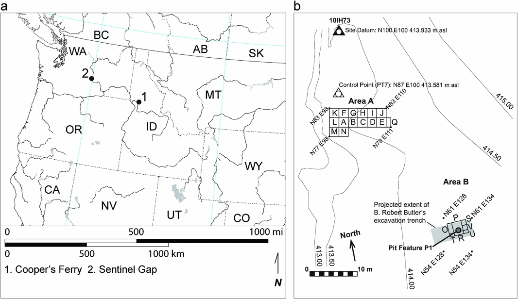
The Cooper's Ferry site is located on an alluvial terrace positioned about 10 m above the confluence of Rock Creek and the lower Salmon River approximately 17 km south of the town of Cottonwood in western Idaho (Figure 2). In 1997, Davis directed the excavation of a 2-×-2-m test unit (Unit A) and encountered a circular pit feature, Pit Feature A2 (PFA2), which contained four stemmed points and other lithic tools (Davis et al. Reference Davis, Nyers and Willis2014). Most importantly, radiocarbon-dated samples from within the pit and from the paleosurface from which the pit feature originated produced a series of late Pleistocene to early Holocene ages (Davis et al. Reference Davis, Nyers and Willis2014; Davis and Schweger Reference Davis and Schweger2004). The early occupation in Unit A, represented by the basal archaeological component CF1 and PFA2, is of late Pleistocene age (Davis and Schweger Reference Davis and Schweger2004), based on associated radiocarbon ages of 11,410 ± 130 B.P. (TO-7349) and 11,370 ± 40 B.P. (Beta-114949). Davis et al. (Reference Davis, Nyers and Willis2014) provide new radiocarbon evidence that supports the hypothesis that PFA2 was created during the late Pleistocene.
Location map for Cooper's Ferry site: (a) site map of excavation units within Area A and Area B during 2012; (b) the 2012 excavation units in Area B were oriented within the projected spatial extents of Butler's trench (gray rectangle) but related to the provenience control of the site grid. Site map north arrow is aligned to true north.

Block excavations began anew in 2009 in Area A, and, in 2012, in Area B to the east; Area B was opened to reveal the stratigraphic record associated with excavations of the 1960s (Butler Reference Butler1969) so that the artifact assemblage collected there might be integrated with that of current excavations. Excavation in Area B revealed twentieth-century disturbed sediments thought to represent the backfill of Butler's excavation trench and deposits from historic road construction. These disturbed sediments extended downward but stopped ca. 1.0–1.5 m above the basal gravel deposits, probably reflecting the limits of the backhoe Butler employed in his 1960s trench excavation. We explored the remaining undisturbed sediments preserved beneath Butler's trench backfill in 2012, discovering Pit Feature P1 (PFP1), which contained 14 stemmed projectile points. Here we present a study of PFP1 and its archaeological contents and discuss how these stemmed points inform our understanding of WST technology.
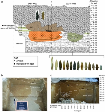
Initially, our 2012 excavations in Area B sought to remove backfilled sediments within Butler's trench to expose his reported stratigraphy (Butler Reference Butler1969). We mechanically excavated a 3-×-4-m block into the eastern portion of Butler's backfilled trench and placed two auger units to establish the total depth of the fill deposit. One of these augers (AU-P1) was placed in excavation Unit P and produced a stemmed projectile point from sediments between 411.10–411.00 m asl. Suspecting that undisturbed archaeological deposits might lie beneath Butler's backfill deposits, we switched to manual excavation and traced out the lower limits of the 1960s excavations. We observed that the modern backfill deposit cut into undisturbed lower silty and sandy sediments that extended ca. 1.0–1.5 m above the basal gravels. Manual excavations into Unit P revealed what appeared to be two pit features, marked by areas of sediment with contrasting color and texture contained in roughly circular plan view shapes; we designated these as Pit Feature P1 (PFP1) and Pit Feature O1 (Figure 3). We will present the results of our investigation of Pit Feature O1 at a future time.
(a) Stratigraphic profiles in Area B of Cooper's Ferry (2012–2013), with position of PFP1 relative to lithostratigraphic and pedostratigraphic units, chronometrically dated samples, and other provenienced artifacts and features. Radiocarbon ages associated with the Rock Creek Paleosol in LU9 from Davis and Schweger (Reference Davis and Schweger2004) and Davis et al. Reference Davis, Nyers and Willis2014; (b) oblique plan view of Pit Feature P1 and Pit Feature O1 matrix fill deposits in stratigraphic context as exposed in process of excavation (view to south); (c) stratigraphic context of PFP1 showing the in situ positions of projectile points (triangles) and debitage (diamonds) as seen from south. Catalog numbers of artifacts are positioned next to symbols; K = krotovina. Southern edge of PFO1 is seen at right in western wall.

Context and Contents of Pit Feature P1
Because the excavations and analysis of the Cooper's Ferry site are currently underway, we can present only preliminary information on the stratigraphic context of feature PFP1 and how these deposits relate to the site's larger stratigraphic framework. Preliminary descriptions of lithostratigraphic units (LU) and pedostratigraphic units (PU) were made from field observations in accordance with methods used by Davis and Schweger (Reference Davis and Schweger2004), Soil Survey Division Staff (1993), Birkeland (Reference Birkeland1984), and NACOSN (1983).
Figure 3 shows a stratigraphic profile of the south and east walls of Area B as they appeared in 2012–2013. Following geoarchaeological methods and frameworks (Davis et al. Reference Davis, Nyers and Willis2014; Davis and Schweger Reference Davis and Schweger2004), we observed 12 different lithostratigraphic units (LU). At the base of the stratigraphic profile, we encountered an angular to subangular cobble gravel deposit and, above this, we observed a stratified series of sandy and silty deposits. Combined with information from the site's other geoarchaeological studies (Davis and Schweger Reference Davis and Schweger2004; Holcomb Reference Holcomb2014), we interpret LU1 to represent alluvial fan gravels originating from the nearby Rock Creek tributary canyon and the sand-dominated deposits of LU2-LU6, LU8, and LU10 to be alluvial point bar deposits. The brown (10YR 5/3) fine sandy loam to loamy sand textures and modest carbonate content of LU7 and LU9 are similar to deposits seen elsewhere in the lower Salmon River canyon and at the Cooper's Ferry site that have been described as aeolian loess (Davis and Schweger Reference Davis and Schweger2004). The LU11 deposit appears to be an infilled alluvial channel that eroded into the site before 9244 ± 36 B.P. This channel is oriented along a northwest to southeast axis and contains archaeological and faunal materials that appear to have been eroded and redeposited from other parts of the site. Poorly sorted backfill deposits from Butler's excavations and the later deposition of other fill deposits are seen in LU12. We encountered a deposit of loamy sand to sandy sediments in the eastern to southeastern excavation units of Area B, which we called Feature V1 in 2012 and 2013 because it retained abrupt boundaries that cross-cut through other adjacent deposits, contained multiple thin (1–2 cm thick) near parallel layers of darker sediment in its lower limits, and many pieces of debitage not associated with rodent burrows. A soil horizon is seen in LU9 bearing weak rubification, carbonate accumulation, massive structure, and elemental geochemistry characteristic of the Rock Creek paleosol observed in Unit A on the site's western side, which is associated with radiocarbon ages of 11,370–11,410 B.P. (Davis et al. Reference Davis, Nyers and Willis2014; Davis and Schweger Reference Davis and Schweger2004; Holcomb Reference Holcomb2014). Although Butler's excavations appear to have truncated the top of PFP1, the color and texture of its infilling deposits is nearly identical to the loesses of LU7 and LU9, which leads us to suspect that the pit was originally excavated downward from the surface of one of these two loess deposits.
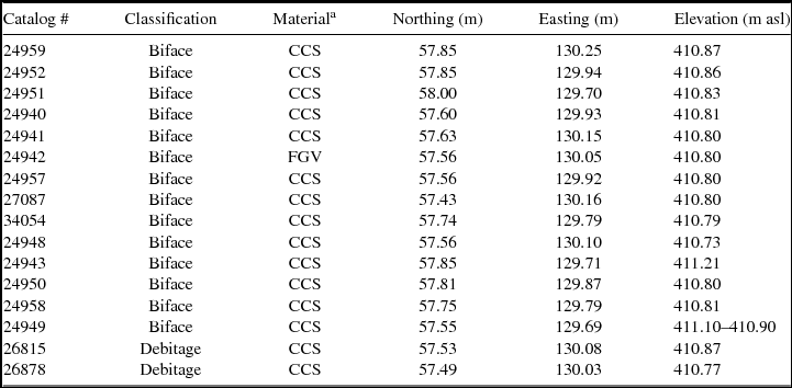
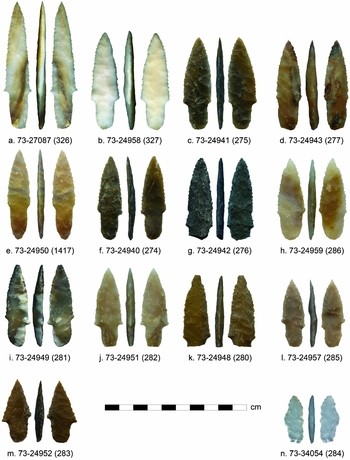
Excavators discovered 14 stemmed projectile points in PFP1, 13 of which were found in situ largely in a 10-cm vertical interval between 411.90–411.80 m asl (Table 1, Figures 3 and 4). Thirteen of the projectile points were of cryptocrystalline silicate; one was of a fine-grained igneous material that is probably basalt. Two projectile points have broken bases (Figure 4g, k) while another has a short, triangular blade that was probably resharpened after its tip was broken (Figure 4m). Generally, these artifacts share similar design qualities: each bears stems with near parallel to gently contracting margins typically ending in rounded to subrounded bases; blades with lengths approximating two-thirds of the projectile point's total length; convex blade margins that sometimes bear fine serrations; bi-convex to plano-convex cross-sections; and some (Figure 4f, i, l, m) bear remnants of an original ventral flake scar. In addition to these 14 projectile points, two pieces of debitage (thin, interior percussion and pressure flakes) were also found in PFP1.
Summary of PFP1 Artifacts.

Note: A systematic error in the surveyed measurement of the Cooper's Ferry site datum was discovered in 2014. A difference of −16.40 m asl was made to this datum and applied to Cooper's Ferry elevation data collected to date.
a CCS = cryptocrystalline silicate. FGV = fine grained volcanic.
Digital images of the 14 stemmed projectile points discovered in PFP1. Catalog numbers and GLiMR numbers (in parentheses) are shown at base of each artifact.

Methods
We used a David SLS-2 structured light scanner to obtain high-resolution (ca. 100 micron) 3D data from the 14 PFP1 points. These 3D point data are exported as a watertight polygon mesh and subsequently split into two faces for further processing in GLiMR (Davis et al. Reference Davis, Bean, Nyers and Brauner2015) and statistical treatment. Discussion of our methods is provided in the Supplemental Text.
Results
The statistics presented in the tables below were generated from a group of nine PFP1 points, which excludes the two broken specimens and the three outliers identified by PCA. The full set of GLiMR data, summary statistics, and metric definitions are provided in Supplemental Tables 1–14. We first describe standard measures, which can be generated through traditional manual measurement and then present novel measures afforded by GLiMR and the more complex 3D Generalized Procrustes Analysis (GPA).
Standard Dimensional and Dimensionless Attributes
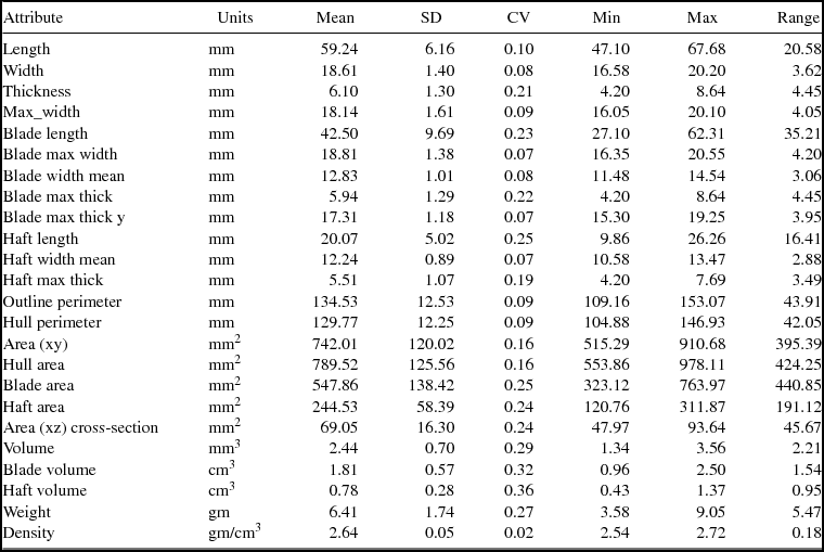
The 14 projectile points range in size from 33.5 to 88.6 mm long, 13.7 to 20.6 mm wide, and 4.2 to 8.6 mm thick; Table 2 provides the basic metrics. Several dimensional measures have low internal variation (as indicated by CV), including length, width, thickness, max width, blade max width, blade width average (i.e., blade area/blade length), blade max thickness Y (the Y coordinate where the blade maximum thickness occurs), haft-width average (i.e., haft area/haft length), outline perimeter (i.e., length of bifacial outline perimeter), hull perimeter (i.e., length of convex hull perimeter), and density (i.e., computed total volume/weight).
Average Dimensional Attributes of PFP1 Points.

Note: Fragmentary and outlier specimens excluded.
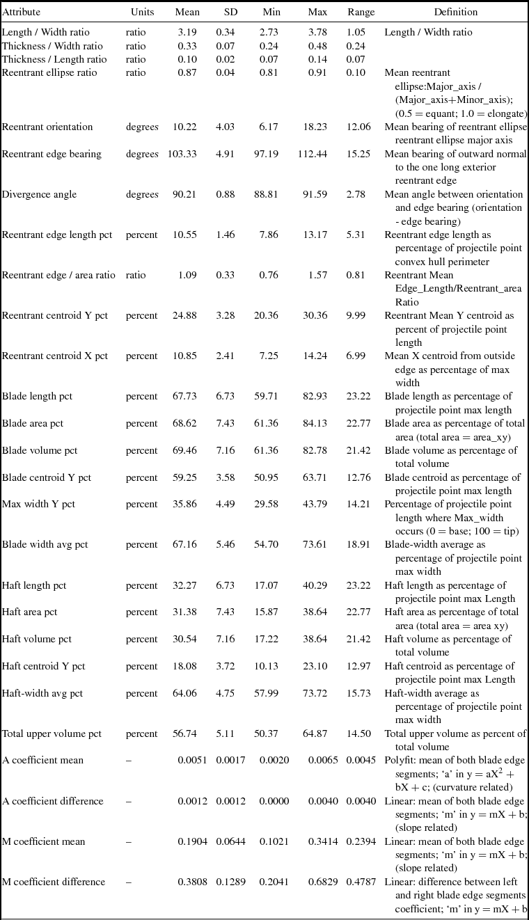
In general, dimensionless metrics of blade and haft sub-domains, ratios, and angular measurements (Table 3) display less variance than dimensional metrics. Many of the dimensionless metrics are expressed as percentages and have a fixed domain from 0 percent to 100 percent. Likewise, most angular measurements have a fixed domain from 0° to 180°. In these cases, directly comparing the standard deviation is appropriate, as these angles do not wrap around zero. Using CV, however, may be misleading given the limited numerical range of some measures. Some of the most diagnostic dimensionless metrics, as evidenced by their low standard deviations, characterize the size, position, and orientation of reentrants. Several dimensionless measures show small standard deviations (≤ 10 percent of mean), including length/width ratio, reentrant ellipse ratio, blade-width average percent (i.e., the average width of blade measures as a percentage of projectile point maximum width), haft centroid Y percent (i.e., the Y position of the haft centroid expressed as a percentage of projectile point maximum length), haft-width average percentage (i.e., haft-width average as a percentage of projectile point maximum width), and total upper volume percent (i.e., the value of the total upper volume as a percentage of projectile point total volume).
Dimensionless and Angular Attributes of PFP1 Points.

Novel GLiMR Measurements
While GLiMR can generate traditional dimensional and dimensionless metric measures rapidly, accurately, and with a high degree of replicability, it can also provide several novel measurements that characterize reentrant attributes (Supplemental Table 15). Because these measures are novel and as yet have no comparators among other WST projectile point populations, we are not certain whether they are significant; however, they may provide useful means of tracking the spatial and temporal distribution of key technological or functional attributes of artifact design.
Reentrant Edge Orientation
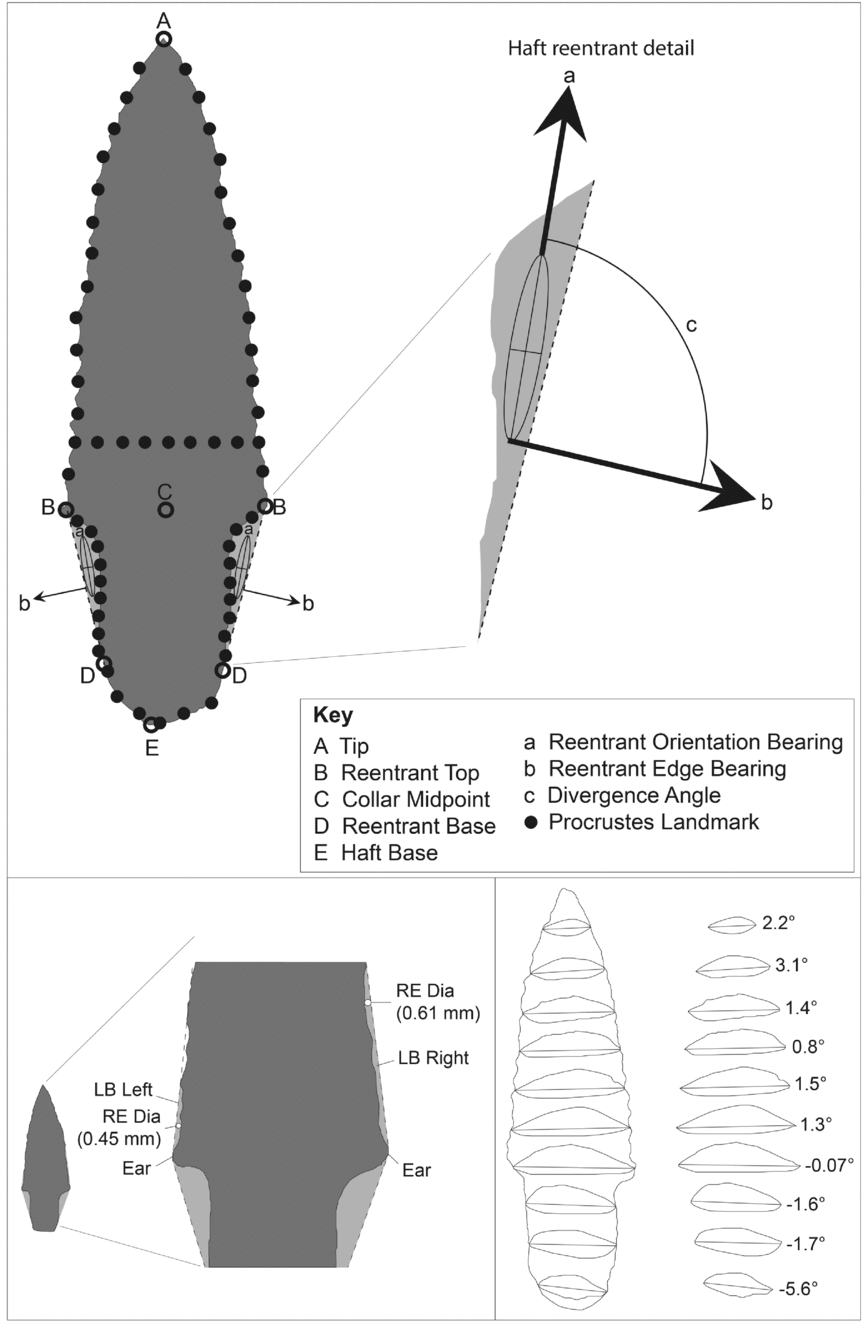
The outermost and longest side of a reentrant is the only side that does not touch the projectile point outline (line BD in Figure 5). Its length is termed Edge_length and the bearing of the outward-pointing normal is termed Edge_bearing (Figure 5b). Bearings are expressed in degrees clockwise from the +Y axis (tip).
Locations of key morphometric measures on PFP1 projectile points: (a–e) key landmark points subdivide perimeter into segments; haft reentrants (light gray) are shown with associated ellipses, axis, and edges; (a–c) haft reentrant angles; (b) reentrant edge bearing is perpendicular reentrant edge BD(dashed line); (a–e) are fixed non-sliding feature-based landmarks established by GLiMR. Solid black circles are initial curve-sliding landmarks that are programmatically set by GLiMR, prior to more comprehensive Generalized Procrustes Analysis. Lower blade reentrants (LB_Left and LB_Right) and “ears” on PFP1 WST projectile point 73–24951 are shown at lower left. Reentrant diameters (RE_Dia) are calculated by GLiMR for reentrants. Transverse cross-section and bifacial midline of multiple XZ planes for PFP1 point 73–24940 and the relative tilt (in degrees) of each bifacial midline and the local amount of axial twist are shown in the inset box at bottom right. Volume for each side, upper (top) and lower (bottom), of a projectile point is calculated by GLiMR as a sum of the area for cross-sections above and below the bifacial midline, taken at 0.05-mm intervals along the Y-axis.

Reentrant Shape and Orientation
Reentrants have shapes that may be equant or elongated and are characterized by standard deviation ellipses approximating the shape of each reentrant. The Ellipse_ratio (major axis/(major axis + minor axis)) quantifies elongation, and its value ranges from 0.5 (equant) to 1.0 (elongate). The Orientation (Figure 5) is the measured bearing of the ellipse major axis and ranges from 0° to 180°. The difference between the Orientation and Edge Bearing is termed the Divergence Angle. It represents the difference between the orientation of the major axis of the reentrant with the normal (i.e., perpendicular) bearing of its external edge. This particular statistic has a narrow range of distribution at ± 0.9° among PFP1 points.
Reentrant Position
The centroids of the left and right haft reentrants represent the position of the reentrant in real coordinates. As such, it is more useful to report their position as a percent of width or length. The widthwise-reentrant position (Reentrant centroid X pct) tracks the location of the haft reentrant centroid as a percentage of how far the centroid lies inboard relative to the total width of the artifact; thus, the average value of 10.9 percent shown in Table 3 indicates that PFP1 points have relatively wide hafts relative to their overall width. The lengthwise reentrant position statistic (Reentrant centroid Y pct) reports the haft reentrant centroid's position along the Y-axis, as measured up from the projectile point's base towards the tip (for PFP1 projectile points and averages to 24.9 percent; Table 3).
Haft Reentrants
Several haft reentrant attributes have tight standard deviations and may help define the 3D GM of WST projectile points from PFP1. The shape, orientation, and position of haft reentrants yield a set of metrics that are characteristic of the points found in PFP1 (Table 3). Of these, Reentrant Edge Bearing (mean 103.3° ± 4.9°), Reentrant Orientation (mean 10.2° ± 4.0°), Divergence Angle (mean 90.2° ± 0.9°), Reentrant Edge Length pct (mean 10.6 percent ± 1.5 percent), Reentrant Ellipse Ratio (mean 0.87 ± 0.04), Reentrant Centroid X pct (mean 10.9 percent ± 2.4 percent), and Reentrant Centroid Y pct (mean 24.9 percent ± 3.3 percent) are values with low standard deviations.
Lower Blade Reentrants
Another set of key reentrants lies along the blade margin just above the boundary between the haft and blade (Figure 5). In addition to area, the size of the lower blade reentrant is measured by GLiMR as the diameter of the largest circle that fits within this reentrant. Among the PFP1 points, this metric spans a range from 0.45 to 1.45 mm for left lower blade reentrants and from 0.45 to 1.35 mm for right lower blade reentrants.
Quantifying Projectile Point Blade Curve Shape
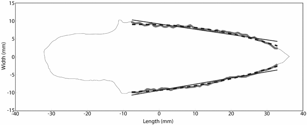
While archaeologists commonly assign nominal characterizations of a projectile point's blade shape (e.g., triangular, excurvate, incurvate, ovate [e.g., Andrefsky Reference Andrefsky2006]), or less frequently from the analysis of 2D landmarks positioned along blade margins (Buchannan and Collard Reference Buchanan and Collard2010), GLiMR fits linear and quadratic curves in the XY plane to digitized blade margins as a means of measuring attributes of slope (M) and a curvature-related coefficient (A; Figure 6 and Table 3). Among the PFP1 points, higher slope values are seen in specimens with shorter “stubby” blades (e.g., Figure 4m and lower slope values associated with longer, “pointy” blades (e.g., Figure 4a). Higher curvature-related values are seen on blades with more convex margin shapes (e.g., Figure 4n, l), and lower curvature values with blade margins approximating straight edges (e.g., Figures 4a, m). Blade margin symmetry is expressed as the difference in slope or curvature-related coefficient of both edges (Table 3) with perfect symmetry near zero and increasing in value with larger asymmetry (e.g., Buchanan Reference Buchannan2006). The most symmetrical blade slope forms among the PFP1 points appear on specimens 73–27087 (0.102), 73–24942 (.143), and 73–24958 (0.156; Figure 4a, g, and b, respectively). The most asymmetrical blade slope forms appear on specimens 73–24952 (0.341) and 73–24957 (0.235; Figures 4m and l, respectively).
Curve fitting analyzes a segment of blade edge (thick gray line) and fits both a linear (thin black line) and second order polynomial (dashed line) curve on specimen 73–24958. Plot axes are zeroed on the projectile point's XY centroid.

Cross-Sections and Thickness as a Continuous Variable
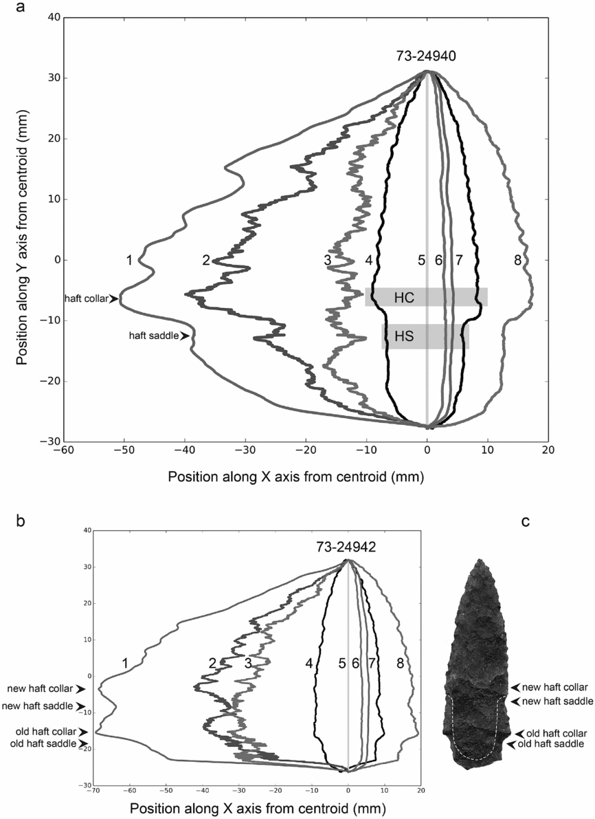
GLiMR calculates transverse cross-sections as 0.05-mm slices taken in the XZ plane. The program divides each cross-section in two along a transverse midline that connects the opposing convergent bifacial edges, producing an upper and lower cross-sectional area. The analyst can then examine cross-section data at any one position or as a continuous variable along the Y-axis. Such an approach to examining the 3D GM form of the PFP1 projectile points reveal attributes that are not revealed by bounding box or single point measurements. For example, Figure 5 shows a graphical output of GLiMR cross-section data for a PFP1 projectile point (Figure 4f), which bears a notable plano-convex shape, as exhibited in its cross-sectional areas above (64.6 percent) and below (35.4 percent) the transverse midline. Cross-sectional measures may be displayed as a continuous variable as well (Figure 7). Examination of cross-sectional data along a projectile point's Y axis reveals this in the greater cross-sectional area of one side (Figure 8a:2) compared to its opposite side (Figure 8a:3). The volume of each side of the projectile point as it lies above and below the transverse midline is calculated by GLiMR and provides insight into the nature of the blank used to create each point. Supplemental Table 3 reports the volumes the projectile points, their upper and lower (larger and smaller, respectively) sides, and the percent volume of a point's largest side (Volume upper pct). Among the PFP1 points, the volume of the largest side ranges from most balanced at 50.4 percent to the most imbalanced at 64.9 percent. Projectile points 73–24940, 73–24957, and 73–24941 have the most imbalanced upper volumes that range from 64.9 percent to 59.4 percent and bear curved longitudinal cross sections. Projectile points 73–24950, 73–24951, and 73–24959 are the most balanced, with upper volumes ranging from 50.4 to 51.1 percent.
Cross-sectional attributes calculated by GLiMR (a) on stemmed point 73–24940: (1) total cross-sectional area (the sum of lines 2 and 3, mm2); (2) upper cross-sectional area component (above bifacial midline mm2); (3) lower cross-sectional area component (below bifacial midline mm2); (4) point outline; (5) Y-axis zero line; (6) lower side maximum thickness (below bifacial midline); (7) upper side maximum thickness (above bifacial midline, mm); (8) total width of outline along Y axis. HC = haft collar. HS = haft saddle; (b) cross-sectional attributes for stemmed point 73–24942 showing morphometric attributes interpreted to signal older and newer haft collar and saddle features; (c) white dashed line overlay shows expected extent of newly manufactured haft element on stemmed point 73–24942.

Scanning electron microscopy images of projectile point 73–24941 (a) from PFP1, showing edge morphology from haft, ear and blade portions, and locations of haft collar and haft saddle; (b) numbers and brackets shown on plan view of projectile point (a) correspond to numbered brackets on top of higher magnification side view of projectile point (b). Haft element is oriented to left on both images.

3D Generalized Procrustes Analysis
Collected 3D landmarks data gathered from the 12 non-broken projectile points were subjected to GPA using the Geomorph package for the R statistical computing platform (Adams and Otárola-Castillo Reference Adams and Otárola-Castillo2013). TPS format 3D landmark data files created via GLiMR were input and analyzed using curve and surface sliding GPA (Gunz and Mitteroecker Reference Gunz and Mitteroecker2013). For this analysis GLiMR was configured to output 74 landmarks for GPA. Sixty-nine outline landmarks from GLiMR were treated as curve-sliding landmarks, and five internal feature based landmarks were set as fixed, non-sliding landmarks. Closed surface meshes generated from aligned GLiMR XYZ data were then loaded into Geomorph. Subsequently, a projectile point bearing a 3D form closest to the average shape of the 12 non-broken PFP1 points (Figure 4b) was chosen as a template to create an additional set of 300 landmarks. We then applied this set of 300 landmarks as sliding landmarks using a minimized bending energy algorithm to the surfaces of each point being analyzed. We analyzed Procrustes landmarks for outliers by plotting the Procrustes distance of each projectile point against the mean landmark shape. Three projectile points—specimens 73–27087, 73–24952, and 73–34054—were obvious outliers in the analysis (Figure S1). These three outliers were plotted against the mean shape using a thin plate spline graph to show which morphological differences separated these projectile points from the rest of the group (Figure S2). After outliers had been detected, a second GPA was performed without specimens 73–27087, 73–24952, and 73–24948, which allowed a mean shape to be generated without being influenced by these shape outliers. Following this second GPA, we performed a principal component analysis (PCA) on Procrustes landmark coordinates. PCA eigenvalues revealed that the first two components accounted for 53 percent of the variation within the dataset and the first four components accounted for 83 percent of all shape variation (Figure S3). We computed a warp grid based on the first two principal components and plotted deformation grids for theoretical component minimums and maximums to help interpret how shape aspects relate to the principal components. Accordingly, principal component one is positively correlated to decreased haft length (i.e., increasing values indicating shorter hafting elements) and increased haft-collar symmetry. Principal component two is positively correlated with imbalanced total upper volume, likely reflecting the production of projectile points from plano-convex blades or linear flake blanks (Figure S4).
Discussion
Traditional Measures
The PFP1 points retained length/width ratios (max 3.78, min 2.73, mean 3.19, SD 0.34) that are comparable to Odell and Cowan's (Reference Odell and Cowan1986:205) experimental assessment that “[p]oints with low length:width ratios tended to last longer in the system (i.e., to incur less damage)” than long and thin projectile points. The PFP1 points also retained thickness/length ratios (max 0.14, min 0.07, mean 0.10, SD 0.02) that approximate the most durable forms measured in Cheshire and Kelly's (Reference Cheshire and Kelly2006) experiment.
GLiMR Measures
Using GLiMR, the 3D GM analysis of the PFP1 projectile points presented here identified several novel measures and patterns that have potential technological implications worthy of further study. Our analysis shows that most of the stemmed projectile points from PFP1 retained imbalanced cross-sections and upper/lower volumes, which we interpret as the result of being produced from linear macroflake blanks and not by extensive multistage bifacial reduction of larger blanks into finished hafted bifaces. In some cases, the presence of the original ventral flake scar surface and a convex longitudinal profile strongly suggests that some specimens were made in this particular fashion. Other specimens that lack these more obvious features might still have been manufactured from blades or linear macroflakes. This interpretation could be tested through an experiment using pressure flaking to create stemmed projectile points similar to the average form of PFP1 specimens from prismatic blades and/or linear macroflakes that are only slightly larger than the average point form. Subjecting the initial experimental blade/flake blank and also the finished projectile points to 3D digital scanning and GLiMR analysis would allow for the calculation of the total upper volume-percent metric. The validity of this test could be rejected if the total upper volume-percent values of experimental projectile points depart significantly from their initial blade/flake blank form and consistently approximate 50.0, thus demonstrating that volumetric imbalance was not necessarily controlled by the projectile point's initial preform shape.
First introduced by Davis et al. (Reference Davis, Bean, Nyers and Brauner2015) as a GM attribute for projectile points, reentrants show promise as a means of characterizing and comparing WST projectile points from Cooper's Ferry. The lower blade reentrant, which was present in all of the PFP1 specimens, may represent a useful index for retouch if the diameter of the lower blade reentrant can be shown to increase in size as a user resharpened a hafted stemmed projectile point's blade. Several measures of the haft reentrant show close metric agreement within the PFP1 point population. These include the angular measures of the Ellipse Ratio (mean 0.87, SD 0.04), the Reentrant Edge Bearing (mean 103.33, SD 4.91), and the Divergence Angle (mean 90.21, SD 0.88). Since these three metrics characterize the form, orientation, and symmetry of the space (i.e., reentrant) created to manufacture the stemmed hafting element, their low range of variation may reflect the intention of their creator(s) to closely replicate key morphometric attributes associated with hafting element design.
The measurement of blade shape via curve fitting could be used to measure the degree of projectile point retouch. In cases where a blade tip was broken, the repair needed to resharpen the projectile point is expected to produce a more extreme blade slope, like that seen in specimen 73–24952 (Figure 4m). Given its relatively high lower blade reentrant diameter (1.4 mm), specimen 73–27087 (Figure 4a) appears to have been resharpened more than other PFP1 points. We interpret the presence of pronounced “ears” that remain at the lateral margins of the haft collar, where the haft transitions to the blade element, to represent the unworked remnants of the original blade margins that escaped resharpening retouch, probably because they were bound with sinew at the upper limit of the hafting element. Because of this, we expect that the size of the lower blade reentrant, which is measured as the diameter of the largest circle that fits within this reentrant, may correlate to the amount of blade resharpening that has occurred during a projectile point's use life.
While a sharp blade margin on a projectile point serves the purpose of achieving greater penetration (Odell and Cowan Reference Odell and Cowan1986) and inflicting additional lacerating damage to fleeing prey after a successful hit, a hafted projectile point can also be used as a knife to butcher a carcass following a kill. In either case, WST hunters undoubtedly found it advantageous to maintain sharp blade margins by performing edge retouch, which led to the gradual reduction in blade width over time. We hypothesize that the lower blade reentrant metric may measure this process of blade resharpening: successive rounds of pressure flake removal to repeatedly resharpen the blade's edge will increase the size of the lower blade reentrant. Conducting an experiment wherein hafted stemmed point replicas are subjected to multiple rounds of 3D scanning and blade margin resharpening could shed light on the validity of this idea. We predict that the size of the lower blade reentrant will be positively related to the number of resharpening events, to a degree that this particular reentrant might be used as a proxy for the use life of a stemmed projectile point. Collecting such data from WST projectile points could shed light on early patterns of tool use, reuse, and discard. The use of lower blade reentrant measures could provide a different (and automated) way to estimate WST projectile point curation (sensu Shott Reference Shott1996) in a conceptually similar way as Ballenger's (Reference Ballenger2001) expended utility index (Shott and Ballenger Reference Shott and Ballenger2007).
By examining the variation in cross-sectional area as a continuous variable along the Y-axis, novel 3D GM attributes are revealed. The quantification of the volume for each side of a projectile point (above and below the bifacial midline) provides a novel means of quantifying the relative balance of cross-sectional symmetry. Several of the PFP1 projectile points retain moderately imbalanced cross-sectional volumes that suggest they were made on blades or linear macroflake blanks, whereas others possess more evenly distributed cross-sectional volumes, which may indicate they were made from larger, more volumetrically balanced blanks. We observe that among the PFP1 projectile points, the part with the largest total cross-sectional area typically lies at the transition between the haft and blade elements, at a position we call the haft collar (Figures 7a:1 and 7a:2 at Y-axis position −7 mm to −9 mm). Maintaining the thickest part of the stemmed projectile point at the haft-blade transition might have served to strengthen the projectile's ability to resist fracturing when subjected to bipolar compression stress during impact with a target. In this way, the haft collar might have acted as a load-bearing buttress, particularly if it was seated just above the distal limit of an organic foreshaft, transmitting some of the force of impact away from the stemmed haft element and into parts of the foreshaft.
Below the haft collar, in the part corresponding to the transition from the blade to the haft element, the total cross-sectional area often reduces abruptly (see Figures 7a:1 and 7a:2 at Y-axis position −12 mm to −15 mm), then increases slightly, and finally reduces in area toward the base of the haft. We call this abrupt reduction in cross-sectional area at the top of the stemmed haft element the haft saddle. The haft saddle is not simply an inevitable by-product of knapping a stemmed haft element. Although retouching the margin of a biface to create a narrower stemmed hafting element will change the local width and cross-sectional area, the haft saddle is further distinguished by an additional reduction in thickness (Z-axis) due to the removal of more substantial flakes across the upper and lower faces. This pattern can be seen in Figure 7a, where upper and lower faces retain marked reductions in their cross-sectional area (i.e., lines 1–3 at Y −10 mm to −15 mm) yet show no significant variation in overall width compared to adjacent portions of the haft (i.e., line 8 from Y −10 mm to −20 mm). Because we see the presence of the haft collar and haft saddle attributes on all but one of the WST projectile points from PFP1 (this feature was lacking in specimen 73–34054), we surmise that the knapper(s) that created these items took care to ensure that the portion with the largest cross sectional area (i.e., widest and thickest) would fall along the transition between the haft and blade elements (at the haft collar) and that the upper portion of the haft would have an abrupt reduction in cross sectional area and thickness (at the haft saddle). The creation of the haft saddle was accomplished by removing one or more longer and thicker flakes from the haft edge margin across one of both faces just below the haft collar (Figure 8). In several cases, the removal of the haft saddle flake(s) appears as overface flake scars (i.e., extending to or past the Y-axis centerline of a projectile point face), which we take as further evidence for the special intention of this morphometric attribute.
We think that the haft saddle may have served one or more functions. First, it may have been created to enhance the union between a projectile's lithic hafting element and an organic foreshaft. The transverse linear depression formed by flaking the haft saddle may have provided an accommodation space that foreshaft material could be pressed into, locking the projectile point stem into the fork of a split stick foreshaft haft, perhaps a bone “clothes pin style” as seen at the Sentinel Gap site (Figure 1; Gough and Galm Reference Gough and Galm2002). Modifying the haft element of a stemmed projectile point to fit tightly within the spatial tolerance of an organic foreshaft was probably more preferable than modifying the organic haft, given that durable organic haft elements were harder to make and might be expected to survive intact longer than stone projectile points (Keeley Reference Keeley1982; Spencer Reference Spencer, Hester, Mildner and Spencer1974; Zeanah and Elston Reference Zeanah and Elston2001). Second, users might have created the haft saddle on PFP1 points to establish a weak point that would cause a fracture at the top of the hafting element during use as a hunting weapon. As others have argued for notched projectile points, the blade portion would detach and remain inside the animal, enhancing its lethality (Ellis Reference Ellis and Knecht1997; Flenniken Reference Flenniken, Plew, Woods and Pavesic1985; Flenniken and Raymond Reference Flenniken and Raymond1986; Musil Reference Musil, Aikens, Willig and Fagan1988; Odell and Cowan Reference Odell and Cowan1986; Titmus and Woods Reference Titmus and Woods1986; Towner and Warburton Reference Towner and Warburton1990; Zeanah and Elston Reference Zeanah and Elston2001).
The co-occurrence of a haft collar and haft saddle is seen in all but one (73-34054) of the PFP1 points,Footnote 1 indicating that it is a common design element of these artifacts. Specimen 73–24942 is unusual as it bears a broken haft element that appears to have been in the process of repair before placement in PFP1. This projectile point's cross-sectional data (Figure 7b, c) reveal what appears to be a double set of haft collar-haft saddles. We believe this reveals a process by which a stemmed point with a broken haft might be repaired. Using a pressure flaker, the manufacturer first removed an initial series of thinning flakes across the face of the haft below a selected point on the blade margin; additional flaking removed the remnants of the old haft collar and saddle and brought the margin of the haft in line with some geometric expectations (shown in Figure 7c). However, in the case of 73–24942, the point was not finished, leaving behind key elements of what we believe is an incomplete haft repair. The discovery and measurement of the haft collar and haft saddle attributes are compelling, and they may be common aspects of WST projectile points. We hypothesize that the WST projectile point haft collar and haft saddle served to enhance the functionality of WST projectile points.
3D Generalized Procrustes Analysis
The 3D GPA analysis reveals that most of the PFP1 points have a narrow range of 3D shape variation and that the strongest influences on variance are due to the influence of volumetric imbalance above and below the bifacial midline and to how close the haft collar is perpendicular to the projectile point's long (Y) axis. We surmise that the volumetric imbalance that exists between the two sides of any particular PFP1 point is probably related to the shape of the initial preform: projectile points made on blades or linear flake blanks lacked sufficient mass to enable the creation of forms with more balanced biconvex cross sections. Moreover, that some projectile points retain varying degrees of longitudinal curvature (e.g., Figure 4a, f) is further evidence that PFP1 projectile points were made on blades and/or linear macroflake blanks. That the long axis curvature and cross-sectional form of PFP1 points are so varied suggests that some were probably manufactured from thicker flake spalls that required relatively more extensive bifacial reduction but also that some were made on thinner blades/linear macroflakes that required relatively less bifacial reduction. We expect that unpredictable nodule shapes and knapping performance of local cryptocrystalline silicates and fine-grained volcanic toolstones may have influenced this variance in bifacial blank shape. In situations where knappers could use toolstones that were well suited to produce adequate blades/linear macroflakes, we anticipate that they might have achieved greater efficiency in the conservation of toolstone and reduced manufacturing effort when creating WST projectile points.
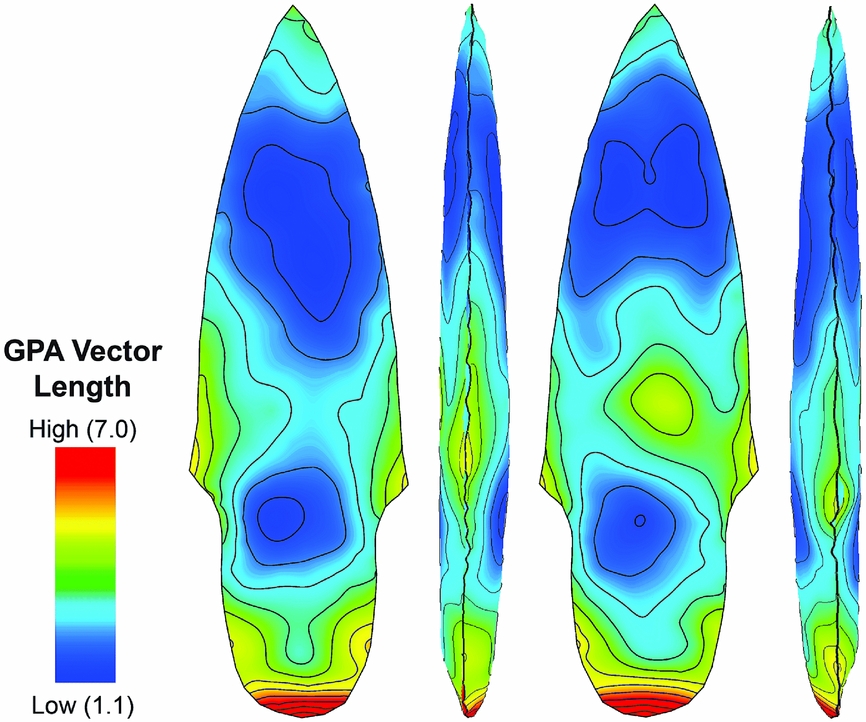
The results of 3D Procrustes Distance analysis show a remarkable degree of similarity in form among the PFP1 point analytical group that we interpret to reflect a corresponding high degree of accuracy and precision in their manufacture. The repeated creation of key design attributes in the same places within tight metric tolerances is evidenced by low Procrustes Distance measures in the areas of the haft saddle and the distal half of the blade element (Figure 9; Figure S5). The 3D Procrustes Distance values are more variable in other areas of the PFP1 points, with the greatest differences in form corresponding to the base of the haft and in the area of the haft collar. We think this shows that there were specific design requirements for PFP1 point blade tips and haft saddles that had to be maintained within tight 3D GM tolerances, whereas other parts could vary much more widely in shape. As well, the high degree of variation in form among the basal portion of haft elements may be caused by damage and subsequent repair of the projectile point during its use life.
3D Procrustes Distance among PFP1 point landmarks as seen in plan and side view. GPA distance data are draped on mean GPA form of PFP1 points. Areas with low GPA distance (blues) share closer spatial agreement (XYZ position) among landmarks than those areas with high GPA distances (yellow, orange, red), which denote areas with greater 3D GM variation.

Because of their widespread appearance, we are curious to know whether the presence of the haft collar and haft saddle were functional design attributes of PFP1 points, perhaps functioning to create a stronger, more stable union between the point's hafting element and the receiving end of an associated organic weaponry system.
Comparing PFP1 with Other Early Projectile Point Caches
Kilby and Huckell (Reference Kilby, Huckell, Graf, Ketron and Waters2013) review interpretations of Clovis artifact caches as ritual offerings, collections of instructional materials for novices, or as a provisioning strategy in material-poor or unfamiliar landscapes. Most of the toolstones used to create the PFP1 points are from high-quality local cryptocrystalline silicates, which is partially consistent with Clovis caches; however, this material is commonly available in the lower Salmon River canyon and the additional presence of a single example made on basalt/andesite is contrary to the Clovis pattern. The PFP1 points bear evidence of having been used and resharpened prior to their burial, which contrasts with the pattern typically seen in Clovis caches that often contain oversized, unused, or unfinished bifacial tools. At face value, the internment of 14 stemmed projectile points in a pit at the Cooper's Ferry site cannot be clearly understood as a ritual feature. Instead, PFP1 appears to have served a more functional role as an equipment cache, similar to nearby PFA2 (Davis et al. Reference Davis, Nyers and Willis2014).
Conclusions
Our findings support the hypothesis that WST projectile points were often made on blades or linear macroflake blanks (Davis et al. Reference Davis, Willis, Macfarlan and Rhode2012, Reference Davis, Nyers and Willis2014). Confirming this hypothesis is important because it reinforces the idea that there was a significant difference in the manufacturing traditions of WST and other Pleistocene-aged projectile points. Many of the Cooper's Ferry WST projectile points were created by pressure flaking a linear macroblade or macroflake blank that was only slightly larger than the final product (Davis et al. Reference Davis, Nyers and Willis2014), whereas early Paleoindian projectile points are thought to be made almost exclusively through the extended percussive reduction of a bifacial preform into a more refined, hafted biface (Bradley et al. Reference Bradley, Collins and Hemmings2010; Davis et al. Reference Davis, Willis, Macfarlan and Rhode2012). This is not to say that other kinds of WST projectile points were never manufactured through more extensive reduction of bifacial preforms (e.g., Beck and Jones Reference Beck and George2010). Indeed, our data hints that some of the PFP1 points were made from larger preforms than others, resulting in artifacts with more balanced volumetric cross-section shapes. Most importantly, however, our study demonstrates that the concept and process of manufacturing projectile points from macroblades and/or macroflakes may be a signature element of the WST. To our knowledge, we provide the first descriptions of the unique 3D GM attributes we call the haft collar and haft saddle. We are curious to know whether these attributes escaped detection before now because traditional, non-digital, manual means of measuring artifact 3D GM were unable to discern such features or whether they are simply novel attributes of the PFP1 artifacts at the Cooper's Ferry site. Although subtle, we believe these attributes are meaningful and, because they consistently appear in the 3D GM of PFP1 points, were created intentionally for a functional benefit and are not simply the inevitable outcome of creating a projectile point, stemmed or otherwise.
Acknowledgments
This research was conducted with permission under Cooperative Agreement L14AC00232 held between the Bureau of Land Management and Oregon State University. Financial support for this research was provided by the Bureau of Land Management, the Keystone Archaeological Research Fund, the Bernice Peltier Huber Charitable Trust, and from the National Geographic Society. David Sisson of the BLM-Cottonwood Field Office provided much appreciated logistical and administrative support. Special thanks to the Nez Perce Tribe for their continued interest and support of our research. We thank the editor and three anonymous reviewers who provided many useful comments and suggestions.
Data Availability Statement
The artifact collection described in this paper is curated in the Cooper's Ferry Collection at Oregon State University's Department of Anthropology. Digital datasets, including 3D scan files, used in this study can be accessed at the Oregon State University ScholarsArchive webpage: https://ir.library.oregonstate.edu/xmlui/
Supplemental Materials
Supplemental materials are linked to the online version of this paper, which is accessible via the SAA member login at https://doi.org/10.1017/aaq.2017.9.
Supplemental Text. David SLS-2 3D Scanning Procedure.
Supplementary Figure 1. CF PFP1 variation in GPA outliers.
Supplementary Figure 2. CF PFP1 outliers compared to mean.
Supplementary Figure 3. CF PFP1 GPA Eigenvalues histogram.
Supplementary Figure 4. CF PFP1 PCA warp grid.
Supplemental Table 1. CF PFP1 MS List of PPTs.
Supplemental Table 2. CF PFP1 MS GLiMR Attribute Definitions.
Supplemental Table 3. CF PFP1 MS Whole PPT Measurements.
Supplemental Table 4. CF PFP1 MS Blade and Haft Measurements.
Supplemental Table 5. CF PFP1 MS Curve Measures.
Supplemental Table 6. CF PFP1 MS Mean Haft Reentrant Measurements.
Supplemental Table 7. CF PFP1 MS Haft Reentrant Differences.
Supplemental Table 8. CF PFP1 MS Lower Blade Reentrant Measurements.
Supplemental Table 9. CF PFP1 MS Lower Blade Reentrant Difference Measurements.
Supplemental Table 10. CF PFP1 MS Left Haft Reentrant Measurements.
Supplemental Table 11. CF PFP1 MS Right Haft Reentrant Measurements.
Supplemental Table 12. CF PFP1 MS Left Lower Blade Reentrant Measurements.
Supplemental Table 13. CF PFP1 MS Right Lower Blade Reentrant Measurements.
Supplemental Table 14. CF PFP1 MS 14C Ages.
Supplemental Table 15. Haft Reentrant Attributes for a Variety of Selected Projectile Point Styles.