2.1. Variable topological space robot description

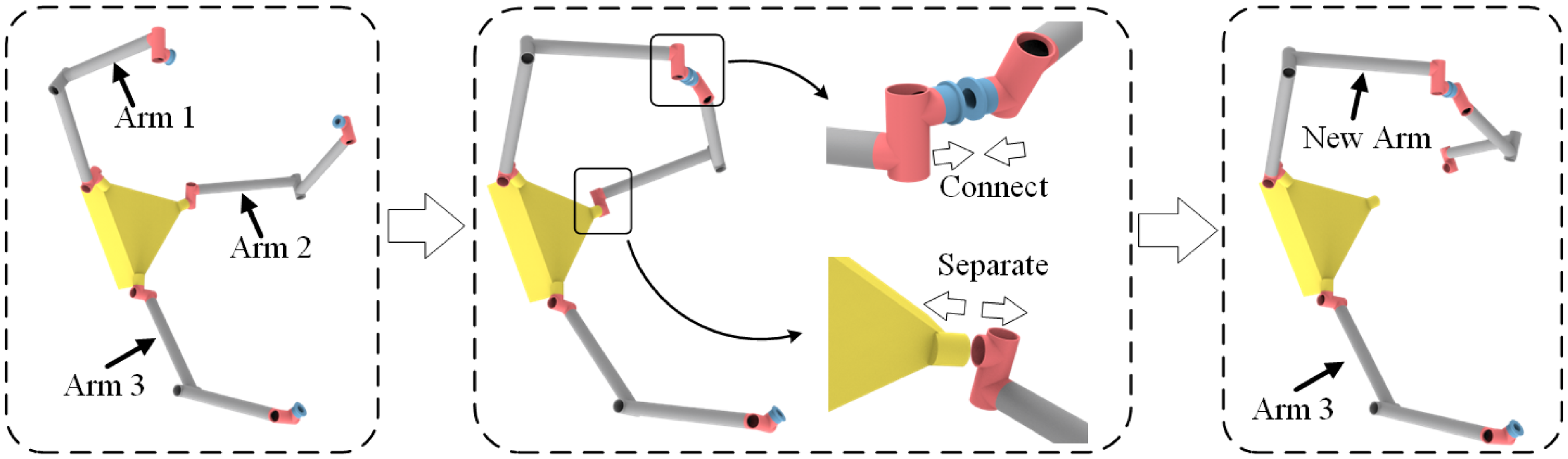
The space robot and its topology transformation process studied in this paper are illustrated in Figure 1. It’s designed as a universal on-orbit operational tool spacecraft, aiming to be applied in numerous scenarios, including the construction of new large-scale space facilities, maintenance of the International Space Station, and the refurbishment and repair of existing defunct satellites, etc. The robot features a base that can translate and rotate in six degrees of freedom (DOFs), operating either under control or freely. It has three arms, each comprising seven links and revolute joints, resulting in 27 DOFs. Here, the triple-arm system is designed to simultaneously accommodate both grasping and manipulation tasks. Besides, it can perform dual-arm cooperative tasks even if one arm is failed. The 7 DOFs in every arm are to ensure that each arm can independently perform tasks within a 6-degree-of-freedom operation space. And the additional 1 degree of freedom ensures the arm can achieve additional functionalities such as obstacle avoidance, singularity avoidance and fault-tolerance control. All components of the robot are treated as rigid bodies. Furthermore, the end of each arm is equipped with a connection mechanism to facilitate topology transformation, enabling it to connect with various links [Reference Malzahn, Kashiri, Romiti, Baccelliere, Cordasco, Laurenzi, Margan, Hoffman, Muratore and Tsagarakis31].

Figure 1.

Diagram of space robot and topology transformation.

To adapt to the variable construction tasks of future space facilities, space robots may need to be able to alter their topology configurations to meet specific task requirements autonomously. One potential scenario is illustrated in Figure 1. The left figure is the initial topology configuration, which is also the configuration unfolded after launch. The workspace or the degree of freedom for the single arm is not large enough for some missions, and there is a need for a more extended arm. Under this circumstance, arm 1 can be separated from the base and connected to arm 2, forming a more extended arm with increased degrees of freedom. To achieve this action, the uncoupled end links of the two arms approach each other and connect when sufficiently close. Subsequently, the root link of one arm detaches from its base, resulting in a “new” single robot with a long, hyper-redundant arm. These coupling/uncoupling operations rely on an advanced connection mechanism that provides mechanical and electrical interfaces, allowing for detachment and attachment on demand. Although extensive research has been conducted on such mechanisms, there is no standard approach or design and each exhibits unique characteristics, making it challenging to describe their dynamic behaviours uniformly. This lack of a standard design or solution underscores the need for a universal dynamic model.

2.2. Dynamic model for link connection

The dynamic model for link connection mainly includes two parts: the space robot dynamic model and the connection process model.

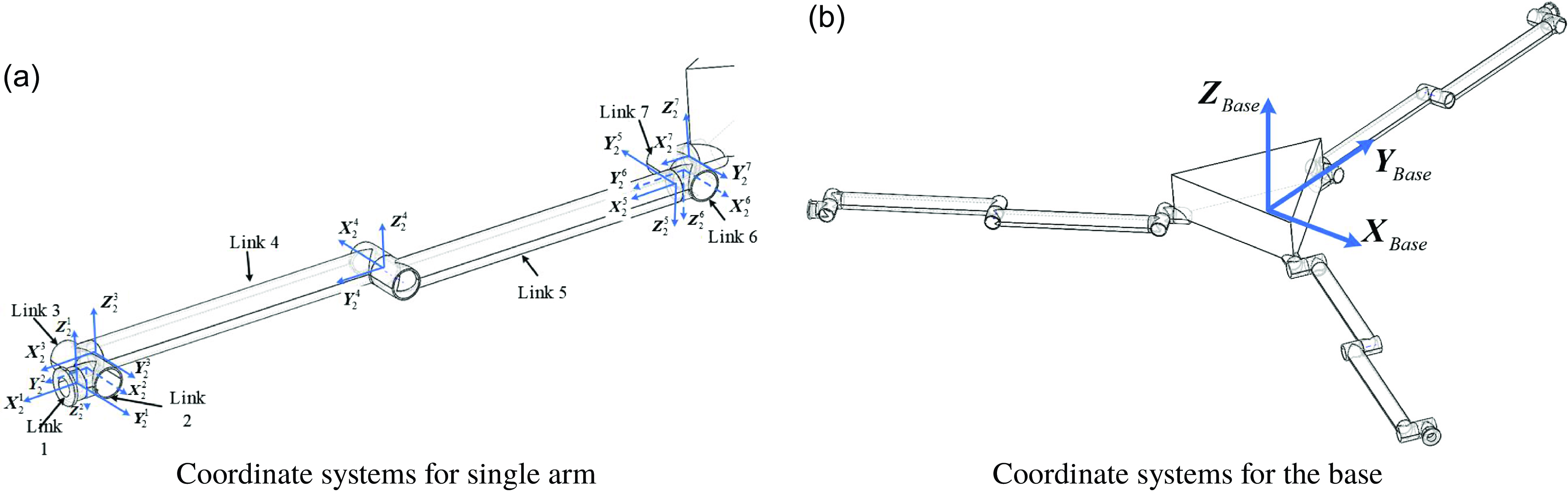
The coordinate system definitions for the robot discussed in this paper are shown in Figure 2. For the definitions of single arm, the links in the arm are numbered in increasing order from tip to base. The $X_{j}^{i}$ denotes the $X$ axis for the $i$ -th link of the arm $j$ . The origin of coordinate system for $i$ -th link is located on the internal hinge. The $X$ axis points to the motion axis, the $Y$ axis points to the external hinge, and $Z$ axis direction is determined according to the right-hand rule. For the coordinate system of the base, the origin is located on its centre of mass, with the axes coinciding with the inertial coordinate system at the beginning.

Figure 2.

Diagram of coordinate systems definition.

The dynamic model of the space robot can be described as follows based on spatial operator algebra [Reference Hu and Wang32]. The velocity, acceleration and force of every joint can be described as:

(1) \begin{equation} V \left ( k \right )=\begin{pmatrix} \omega _{k} \\ v_{k} \end{pmatrix} \end{equation}

(2) \begin{equation} \alpha \left ( k \right )=\begin{pmatrix} \dot {\omega }_{k} \\ \dot {v}_{k} \end{pmatrix} \end{equation}

(3) \begin{equation} f \left ( k \right )=\begin{pmatrix} N_{k} \\ F_{k} \end{pmatrix} \end{equation}

where the subscript $k$ represents the $k$ -th link; $\omega _{k}$ and $v_{k}$ denote the angular and linear velocity vectors of joint $k$ ; $N_{k}$ and $F_{k}$ mean the joint moments and force vectors, respectively.

The velocity and acceleration recursive relationship between adjacent links is:

(4) \begin{equation} \left \{ \begin{array}{rl} V(k)&= \phi ^T(k+1,k)V(k+1) + H^T(k)\dot {\theta }(k), \\ \alpha (k)&= \phi ^T(k+1,k)\alpha (k+1) + H^T(k)\ddot {\theta }(k) + a(k) \end{array} \right . \end{equation}

where $a(k)$ is the Coriolis acceleration term; $\phi (k+1,k)$ denotes the interbody transformation operator; $H(k)$ denotes the joint map matrix; $\theta (k)$ is the vector of generalized variables for the $k$ -th hinge. Specially, the base is connected with inertial space by a virtual hinge, so the $\theta (k)$ for the base denotes both the translation and rotation displacement of the base.

The force and torque recursive relationship between adjacent links is:

(5) \begin{equation} \begin{array}{rl} f(k)= &\phi (k,k-1)f(k-1)+M(k)\alpha (k)+K(k)\theta (k)+D(k)\dot {\theta }(k)+b(k) \end{array} \end{equation}

where $M(k)$ denotes the inertia matrix; $K(k)$ denotes the stiffness matrix; $D(k)$ denotes the damp matrix; $b(k)$ is the centrifugal force term for the $k$ -th body, whose detailed expression can be found in ref. [Reference Jain and Rodriguez33].

The operator expressions for the generalized forces $f= col\left \{\, f(k) \right \}$ and the spatial velocities $V= col\left \{ V(k) \right \}$ of all the bodies in the system are given by:

(6) \begin{equation} V=\phi ^T H^T \dot {\theta } \end{equation}

(7) \begin{equation} \alpha =\phi ^T H^T\ddot {\theta }+\phi ^T a \end{equation}

(8) \begin{equation} f=\phi (M\alpha +K\theta +D\dot {\theta }+b ) \end{equation}

(9) \begin{equation} T_{a}=Hf \end{equation}

Write the these items as the operator expressions, and the dynamic model for the whole system is as follows:

(10) \begin{equation} \begin{array}{rl} T_{a}=&Hf=H\phi M \phi ^T H^T \ddot {\theta }+H\phi K\theta +H\phi D\dot {\theta }+H\phi ( M\phi ^T a+b) \\ =&\mathcal{M} \ddot {\theta }+\mathcal{K} \theta +\mathcal{D} \dot {\theta }+\mathcal{C} \end{array} \end{equation}

Here, $\mathcal{M}$ is the system mass matrix, $\mathcal{K}$ is the system stiffness matrix, $\mathcal{D}$ is the system damp matrix, and $\mathcal{C}$ is the vector of Coriolis and centrifugal forces for the system.

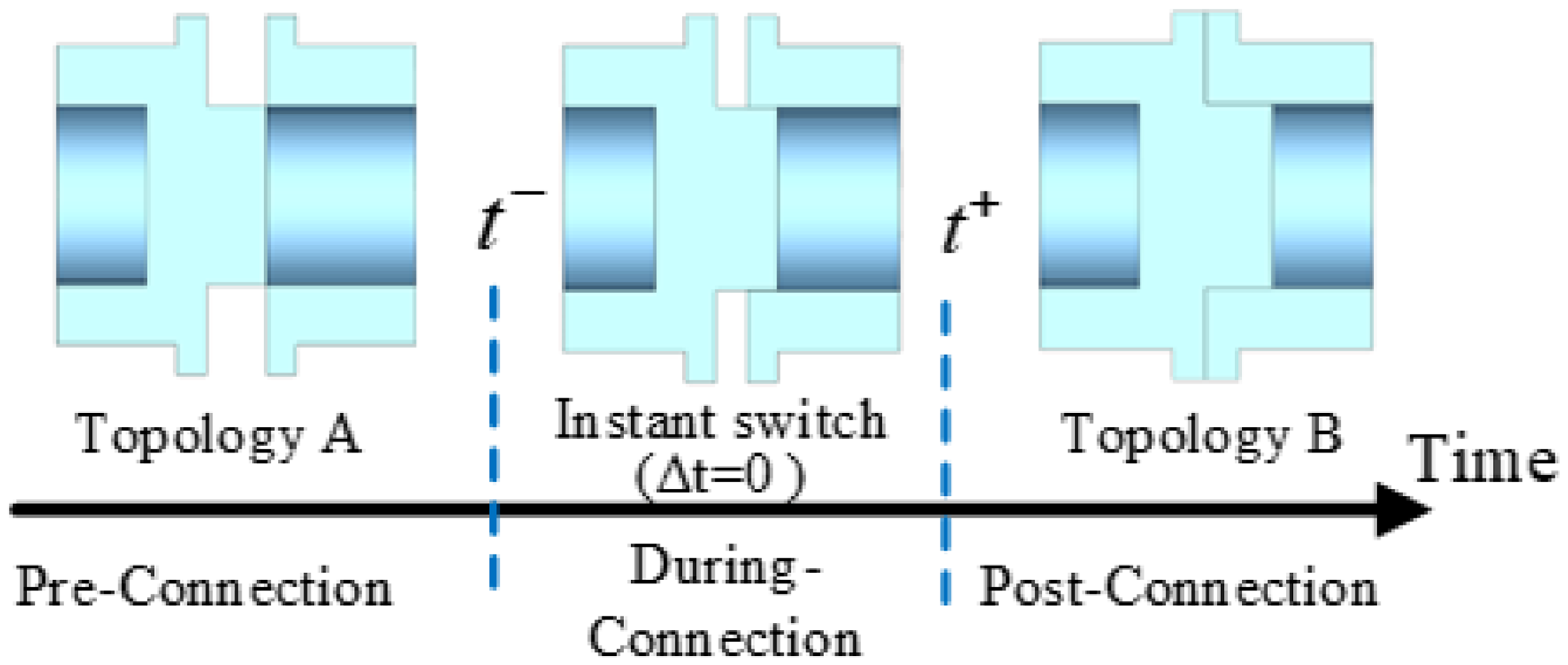
The docking process can be divided into three phases: pre-, during- and post-connection, just as shown in Figure 3. The docking discussed here is only the connection between different modules inside the space robot system. Here, we take a simple probe-cone mechanism as an example. The pre-connection phase indicates the stage just before the probe makes contact with the outer edge of the cone. This remains in the configuration of Topology A. The during-connection shows the stage of the probe’s movement through the cone, where the topology transformation happens. The post-connection indicates the stage after the probe is in full contact with the cone. This becomes a new topology, for example, Topology B. The dynamic behaviours during the pre-connection phase can be described as in (10). The motion occurring during the connection phase is inherently complex, involving movements within the connection mechanism as it transitions from the connection initiation to a stable state. This phase represents a constrained dynamical process highly dependent on the specific design features of the connection mechanism. For analytical simplicity, the during-connection phase is considered to occur instantaneously. Then the dynamic process for this phase becomes a transient impact, which is also the one that needs to be minimized. The impact from reconfiguration just occurs at this moment. Before or after this instance, there is no more impact from this transformation.

Figure 3.

Diagram of docking process.

Before proceeding with the derivation of the dynamic equations, several assumptions need to be introduced:

1. 1) The reconfiguration is assumed to take place at an instant of time, in other words, the short interval $\Delta t$ can be regarded as 0.

2. 2) The generalized coordinates of the system remain unchanged during the reconfiguration. In other words, the joint angles, base position and base orientation do not change. But their velocities may have a sudden jump.

3. 3) The generalized coordinates and the externally applied forces are continuous, and the velocities are bounded during the sudden event.

Given this assumption, the position coordinates remain unchanged, while the system’s velocity changes suddenly, as follows:

(11) \begin{equation} \begin{aligned} \Delta t & \rightarrow 0 \\ \theta ^- = \bar {\theta } &= \theta ^+ = \text{const} \\ \dot {\theta }^- & \neq \dot {\theta }^+ \end{aligned} \end{equation}

Here, $-$ and $+$ represent the start and end moments of an event, respectively.

Under these assumptions, integrate the robot dynamics over the short interval $\Delta t=[t^-,t^+]$ , take limits as $\Delta t$ tends to $0$ , and the following can be obtained:

(12) \begin{equation} \begin{aligned} \lim _{\Delta t\rightarrow 0}\int _{t^-}^{t^+}\left \{ \mathcal{M}\ddot \theta +\mathcal{K} \theta +\mathcal{D} \dot {\theta }+\mathcal{C}\right \}dt =\lim _{\Delta t\rightarrow 0}\int _{t^-}^{t^+}\left \{ T_a-C_{c}^T \lambda \right \}dt \end{aligned} \end{equation}

where $C_{c}$ represents the Jacobian of the constraint equations, and $\lambda$ denotes the Lagrange multipliers. Incorporating the constraint term allows for a more comprehensive description of the system and is essential for deriving the jump in velocities.

Here $\mathcal{M}$ , $\mathcal{K}$ , $\mathcal{D}$ and $C_{c}$ are functions of only generalized coordinates, which means $\mathcal{M}(\theta )$ , $\mathcal{K}(\theta )$ , $\mathcal{D}(\theta )$ and $C_{c}(\theta )$ . Considering that $\theta$ is constant during the integration, then (12) can be expressed as:

(13) \begin{equation} \begin{aligned} \lim _{\Delta t\rightarrow 0} \left (\mathcal{M}(\theta )\Delta \dot \theta +\mathcal{K}(\theta )\theta \Delta t+\mathcal{D}(\theta )\Delta \theta +\int _{t^-}^{t^+}{\left .\mathcal{C}(\theta ,\dot {\theta })dt\right ) =\lim _{\Delta t\rightarrow 0} (\bar {T}_a\Delta t-C_{c}(\theta )^T\mu )}\right . \end{aligned} \end{equation}

In (13), $\mathcal{C}(\theta ,\dot {\theta })$ is a continuous function on the small-scale time interval $[t^-,t^+]$ . Using the mean value theorem for integrals, there is one point $t_{\xi }$ such that:

(14) \begin{equation} \int _{t^-}^{t^+} \mathcal{C}(\theta ,\dot {\theta }) \, \mathrm{d}t = \mathcal{C}(\bar {\theta },\dot {\theta }_{\xi })(t^+-t^-) = \mathcal{C}(\bar {\theta },\dot {\theta }_{\xi }) \Delta t \end{equation}

Then considering the generalized coordinates $\theta$ remain constant at this interval $\Delta \theta \rightarrow 0$ and $\Delta t \rightarrow 0$ . Hence, (13) can be simplified to:

(15) \begin{equation} \mathcal{M}\Delta \dot {\theta }=-C_{c}^T\mu \end{equation}

where $\delta \dot {\theta }$ and $\mu$ are all unknown variables.

Then, we define $C_{c}^-$ and $C_{c}^+$ as the constraint Jacobian matrices before and after the impact switch, respectively. Generally, the constraint equations at the position level must be satisfied at all times during the interval. Thus, the following equations are obtained:

(16) \begin{equation} \varphi ^-(\theta ^-)=0,\: \varphi ^+(\theta ^-)=0,\: \varphi ^+(\theta ^+)=0 \end{equation}

Then, the velocity level constraint equations can be derived by differentiating (16):

(17) \begin{equation} \dot {\varphi }^+(\theta ^+)=C_{c}^+\dot {\theta }^+=0 \end{equation}

Considering $\Delta \dot {\theta }=\dot {\theta }^+-\dot {\theta }^-$ , one obtains:

(18) \begin{equation} C_{c}^+\dot {\theta }^-+C_{c}^+\Delta \dot {\theta }=0 \end{equation}

Associating (15) with (18), the following is obtained:

(19) \begin{equation} \begin{bmatrix} \mathcal{M}(q) & \left [ C_{c}^+ \right ]^T\\ C_{c}^+ & 0 \end{bmatrix} \begin{bmatrix} \Delta \dot {\theta } \\ \mu \end{bmatrix}= \begin{bmatrix} 0 \\ -C_{c}^+\dot {\theta }^- \end{bmatrix} \end{equation}

where, $\Delta \dot {\theta }$ denotes the jump in velocities and $\mu$ denotes the total impulse during connection at the contact point.

2.3. Optimization metrics during transformation

From (19), it can be observed that the impulse is primarily induced by topology changes and the end velocities prior to transformation. However, the end velocities cannot perfectly reach $0$ . Thus, some impulse is unavoidable during topology changes; in other words, an impact is also unavoidable, although potentially small. These impacts occur at every joint and contact point within the system and can lead to irreversible damage, such as the shedding of solid lubrication. This characteristic directly influences space robots’ lifespan; when damage accumulates to a critical threshold, joint failure occurs, rendering the robot incapable of continuing operations. Therefore, minimizing the impact associated with each topology change process is essential for efficiently functioning space robots. Given the difficulties in quantifying the impact force without detailed knowledge of the connection mechanism design, this paper utilizes impulse as the integral of the impact force over time as the optimization metric. To derive the impulse in every joint, integrate (8) over the short interval $\Delta t$ and the following can be obtained:

(20) \begin{equation} L=M_{1} \Delta \dot {\theta } +\lim _{\Delta t \to 0}\int _{t^-}^{t^+} {K}_{1}\theta +{D}_{1}\dot {\theta } +{C}_{1} dt=M_{1} \Delta \dot {\theta } \end{equation}

where $L$ denotes the total impulse in all the joints, ${C}_{1}$ represents all the nonlinear items of every link, including Coriolis forces, centrifugal forces and elastic forces. By substituting the $\Delta \dot {\theta }$ from (19) into the (20), the impulse experienced by all joints during the connection process can be calculated.

For the space robot depicted in Figure 1, each joint is constrained to revolve only around the X-axis within its respective body-based coordinate frame, commonly called the driven direction. Since each joint possesses degrees of freedom to rotate in its driven direction, the impulse applied along this axis will not cause damage; instead, it will result in rotation. Conversely, impulses in non-driven directions are significant sources of potential damage and must be minimized. This requirement can be articulated as follows:

(21) \begin{equation} L(k)=\left [ \begin{matrix} L_{k}^{rx} \\ L_{k}^{ry} \\ L_{k}^{rz} \\ L_{k}^{tx} \\ L_{k}^{ty} \\ L_{k}^{tz} \end{matrix} \right ] \to L{}' (k)=\left [ \begin{matrix} L_{k}^{ry} \\ L_{k}^{rz} \\ L_{k}^{tx} \\ L_{k}^{ty} \\ L_{k}^{tz} \end{matrix} \right ] \end{equation}

So the optimization metrics can be defined as:

(22) \begin{equation} F(\theta )=\Sigma \left \| L{}'(k) \right \|_{2} \end{equation}

3.1. Lower-level optimization model

For the lower-level optimization, the contact position and orientation with respect to the base $x_{0}$ are given. This optimization aims to determine the optimal joint angles to minimize the impulse. These joint angles should satisfy the constraints to ensure the ends reach the specified contact position and orientation. Additionally, they must adhere to self-avoidance constraints to prevent interference among individual links. The range of joint angles is limited to $\left [ -\pi ,\pi \right ]$ . The lower-level optimization problem can be described as:

(23) \begin{align} \text{Min } &f(\theta )=F(\theta ,x_{0}) \nonumber \\ \nonumber \text{s.t. } &\Phi _{c}^{l}(\theta ,x_{0}) =0\\ &\Phi _{o}^{l}(\theta ,x_{0} ) =0\\ \nonumber &\theta _{i}\in \left [ -\pi ,\pi \right ] \end{align}

where superscript $l$ indicates constraints in lower-level optimization; $\Phi _{c}^{l}(\theta )$ represents the constraints that ensure the ends of the two arms achieve the specified contact position and orientation; $\Phi _{o}^{l}(\theta )$ denotes the self-avoidance constraint. $\Phi _{c}^{l}(\theta )$ can be expressed as residuals resulting from the solution of inverse kinematics equations:

(24) \begin{equation} \Phi _{c}^{l}(\theta ,x_{0})=a_{1}\cdot R_{1}+a_{2}\cdot R_{2} \end{equation}

where $R_{1}$ and $R_{2}$ denote the residuals in solving inverse kinematics equations for the two arms, respectively, $a_{1}$ and $a_{2}$ represent close-loop coefficients.

The self-avoidance constraint is formulated using the artificial potential field method. The repulsive force can be calculated as follows:

(25) \begin{equation} \begin{aligned} f_{r}(\theta )=\left \{\begin{matrix} \sum (k_{r}\cdot (\frac {1}{d}-\frac {1}{d_{0}})^{2}) & d\le d_{0} \\ 0 & d\gt d_{0} \end{matrix}\right . \end{aligned} \end{equation}

where $k_{r}$ denotes the repulsion coefficient; $d_{0}$ represents the safety distance threshold. The repulsive force can be directly utilized as the self-avoidance constraint $\Phi ^{l}_{o}(\theta )$ .

Most existing optimization algorithms cannot handle constraints directly. A common method is to reformulate the constraint conditions as penalty terms and incorporate them into the objective function. For the inequality constraint $\theta _{i}\in \left [ -\pi ,\pi \right ]$ , and considering the periodic nature of the joints, when a joint angle exceeds these bounds, it is corrected to fall within the allowable range by adding or subtracting $2\pi$ to it. Then, the lower-level optimization problem can be expressed as:

(26) \begin{equation} \begin{aligned} \text{Min } & f(\theta ,x_{0})=F(\theta ,x_{0})+ \Phi _{c}^{l}(\theta ,x_{0} )+\Phi _{o}^{l}(\theta ,x_{0} )\\ \text{s.t. } & \theta _{i}\in \left [ -\pi ,\pi \right ] \end{aligned} \end{equation}

3.2. Upper-level optimization model

The upper-level optimization aims to determine the optimal contact position and orientation that minimize the impulse. The contact position and orientation are utilized in the lower-level to calculate the minimal impulse, with the optimal value serving as the objective metric in the upper-level. The constraints include ensuring that the contact pose lies within the dual-arm public workspace, thereby making the pose reachable. Additionally, the self-avoidance constraint is incorporated. Thus, the upper-level optimization problem can be formulated as follows:

(27) \begin{equation} \begin{aligned} \text{Min } & f(x)=f_{best}^{l}(x)\\ \text{s.t. } & \begin{array}{l} \Phi _{c}^{u}(x) =0\\ \Phi _{o}^{u}(x) =0 \end{array} \end{aligned} \end{equation}

where $x$ denotes the vector of contact position and orientation, and the superscript $u$ denotes constraints in the upper-level optimization. The term $f_{best}^{l}(x)$ is the optimal value of the lower-level optimization for a given contact pose $x$ ; $\Phi _{c}^{u}(x)$ denotes the constraints to ensure the pose is reachable; $\Phi _{o}^{u}(x)$ means the self-avoidance constraint.

These two constraints are all considered in the lower-level optimization. With well-chosen coefficients, it may not be necessary to consider these constraints explicitly at the upper level. For example, if the contact position and orientation are unreachable, the residuals yield a significant value. Given an appropriately chosen coefficient, the objective metrics become significantly larger than the optimal impulse, automatically excluding unreachable poses. The same applies to the self-avoidance constraint. Consequently, the upper-level optimization problem can be simplified as follows:

(28) \begin{equation} \text{Min } f(x)=f_{best}^{l}(x) \end{equation}

which is an unconstrained optimization problem that is much easier to solve than the original one.

In summary, the bilevel problem can be expressed as:

(29) \begin{equation} \begin{aligned} \text{Min } &f(x,\theta )=F(x,\theta )+\Phi _{c}^{l}(\theta ,x)+\Phi _{o}^{l}(\theta ,x )\\ \text{s.t. } & \theta _{i}\in \left [ -\pi ,\pi \right ] \end{aligned} \end{equation}

4.1. Bilevel optimization solving approach

The model established in Section 3 represents a typical bilevel optimization problem, wherein one optimization task is embedded with another. Consequently, each iteration of the upper-level optimization necessitates solving for the optimal solution of the lower-level optimization. This solution process is computationally intensive and can be exceedingly time-consuming. Additionally, the problem is strongly coupled and highly nonlinear, complicating the search for an optimal solution. The most common approach to addressing a bilevel problem involves reforming it into an equivalent single-level problem. This is achieved based on the necessary and sufficient conditions of Karush Kuhn Tucker associated with the lower-level problem [Reference Camacho-Vallejo, Corpus and Villegas34]. However, this reformulation is only feasible when the lower-level problem is convex, and this cannot be applied to the non-convex problem presented in this work. Moreover, it is also impossible to transfer the problem into a single-level one. Because this will lead to the solution being stuck in local optimality, as discussed in Section 3.

Classical methods make it hard to solve the problem proposed due to their high nonlinearity and non-convexity. However, heuristic algorithms are well-suited to solving bilevel problems owing to their advantages in handling nonlinearities and achieving computational efficiency. This work employs PSO [Reference Liang, Guo, Chen, Yu, Yue and Li35] to solve the lower-level optimization problem and find the global optimal solution. At the same time, the SA method is utilized for the upper-level optimization to enhance solving speed. For lower-level optimization, the objective function is represented as (26), an unconstrained optimization problem where coefficients can adjust the penalty degree. The PSO algorithm randomly searches each particle based on swarm intelligence. In $n$ -dimensional optimization space, the individual position and velocity of the $i$ -th particle are denoted as $q(i)=\begin{pmatrix} q_{1}(i),&q_{2}(i),& \dots &q_{n}(i)\end{pmatrix}$ and $v(i)=\begin{pmatrix} v_{1}(i),&v_{2}(i),& \dots &v_{n}(i)\end{pmatrix}$ , respectively. The individual optimal position for the $i$ -th particle is $q_{best}(i)$ , and the global optimal particle position is denoted as $q_{global}$ . The update strategy for the particle is as follows:

(30) \begin{equation} \left \{ \begin{aligned} v_{k+1}(i) & = \mu v_{k}(i) + c_{1}r_{1}(q_{best}(i) - q_{k}(i)) + c_{2}r_{2}(q_{global} - q_{k}(i)), \\ q_{k+1}(i) & = q_{k}(i) + v_{k+1}(i) \end{aligned} \right . \end{equation}

where $c_{1}$ and $c_{2}$ are learning factors; $r_{1}$ and $r_{2}$ are random numbers between 0 and 1; $\mu$ is the inertia weight factor.

The update process in the PSO algorithm incorporates both the individual optimal values and the global optimal value, thereby endowing it with robust global search capabilities. Furthermore, as particles share each other’s best experiences – namely, their individual best positions and the global best position, PSO can rapidly converge on improved solutions. The interactions among particles influence their positions, enhancing the search process’s overall efficiency. Consequently, PSO is employed as the solving algorithm for lower-level optimization to identify the global optimal solution effectively.

In the upper-level optimization, the objective function, defined in (28), is structured as an unconstrained optimization problem. The penalty level can be fine-tuned by adjusting coefficients within the penalty terms. Given the computationally intensive nature of bilevel optimization, the upper-level algorithm should operate efficiently with minimal steps to accelerate the overall solving process. Unlike PSO, which requires multiple evaluations per step, simulated annealing (SA) calculates the objective function only once per iteration, making it more suitable for the upper-level optimization. SA finds the global optimal solution using the Metropolis principle [Reference Delahaye, Chaimatanan and Mongeau30], which probabilistically accepts new states rather than relying solely on deterministic rules. This acceptance probability is represented as:

(31) \begin{equation} P=\left \{\begin{matrix} 1, & f(k+1)\lt f(k)\\[3pt] e^{-\frac {f(k+1)-f(k)}{\vphantom{\frac{1}{2\frac{1}{2}}}T} }, & f(k+1)\ge f(k) \end{matrix}\right . \end{equation}

In general, simulated annealing algorithms work as follows. The temperature progressively decreases from an initial positive value to zero. At each time step, the algorithm randomly selects a solution close to the current one, measures its quality, and moves to it according to the temperature-dependent probabilities of selecting better or worse solutions, which during the search respectively remain at 1 (or positive) and decrease toward zero.

4.2. Optimization results

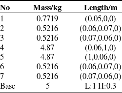
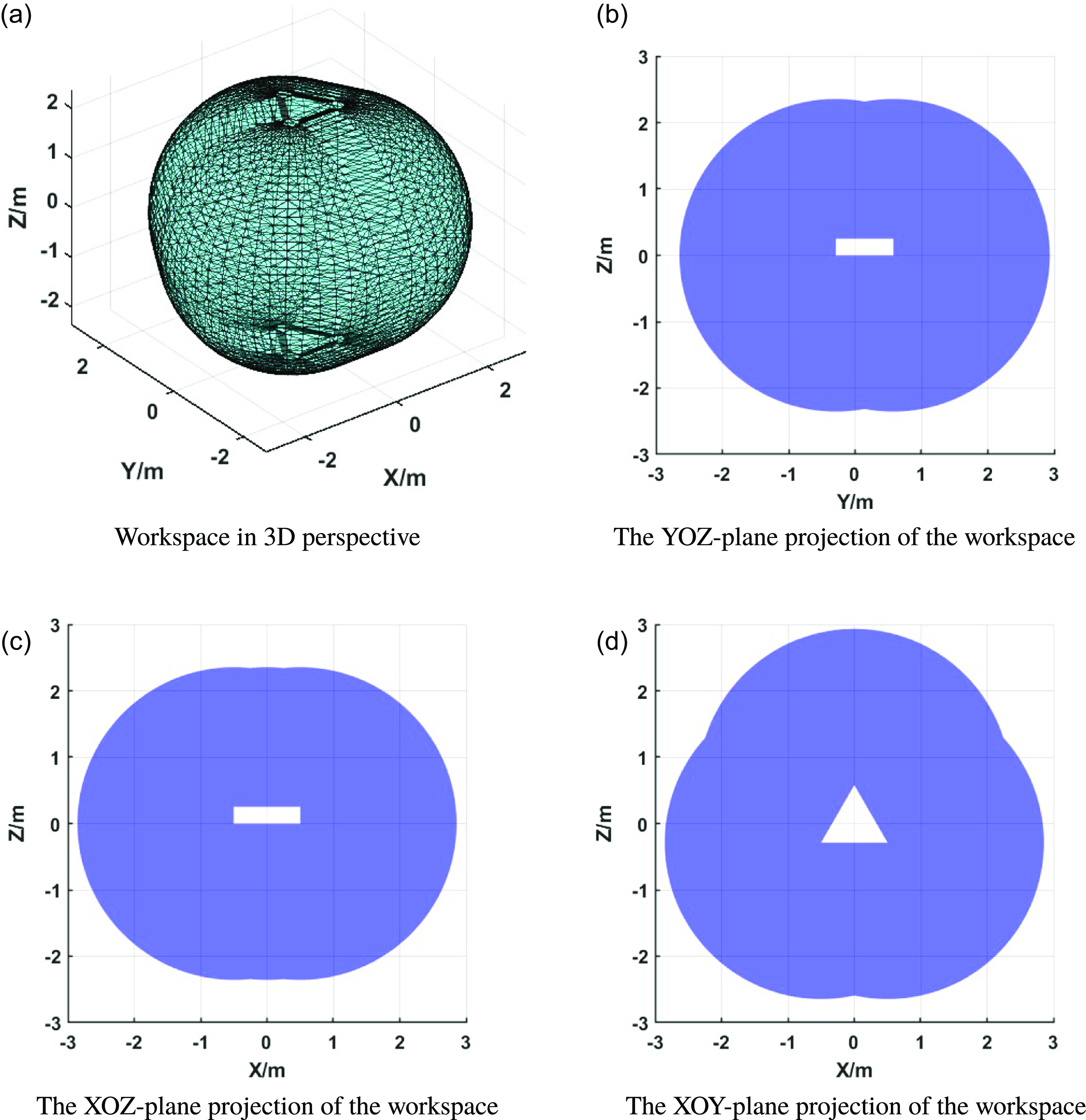
In this subsection, the optimization problem in Section 3 is solved with the algorithm in Section 4.1. The detailed parameters of the space robot employed are shown in Table I. Here, the No means the link number, as shown in Figure 2. The length for the base means the base refers to a triangular prism with sides 1 m long and 0.3 m high. The link parameters listed are those of links in arm 1; the parameters for arm 2 and arm 3 are the same. If the base is fixed, the workspace for this space robot is shown in Figure 4. Considering there are no more constraints on the robot, the workspace for each arm is a sphere centred at the installation point of the arm on the base, with a radius equal to the maximum reach of the arm. Additionally, the volume occupied by the base must be subtracted from this sphere. And the whole workspace for the system is the union of the workspaces of all individual arms.

Table I.

Parameter for space robot.

Figure 4.

Diagram of workspace.

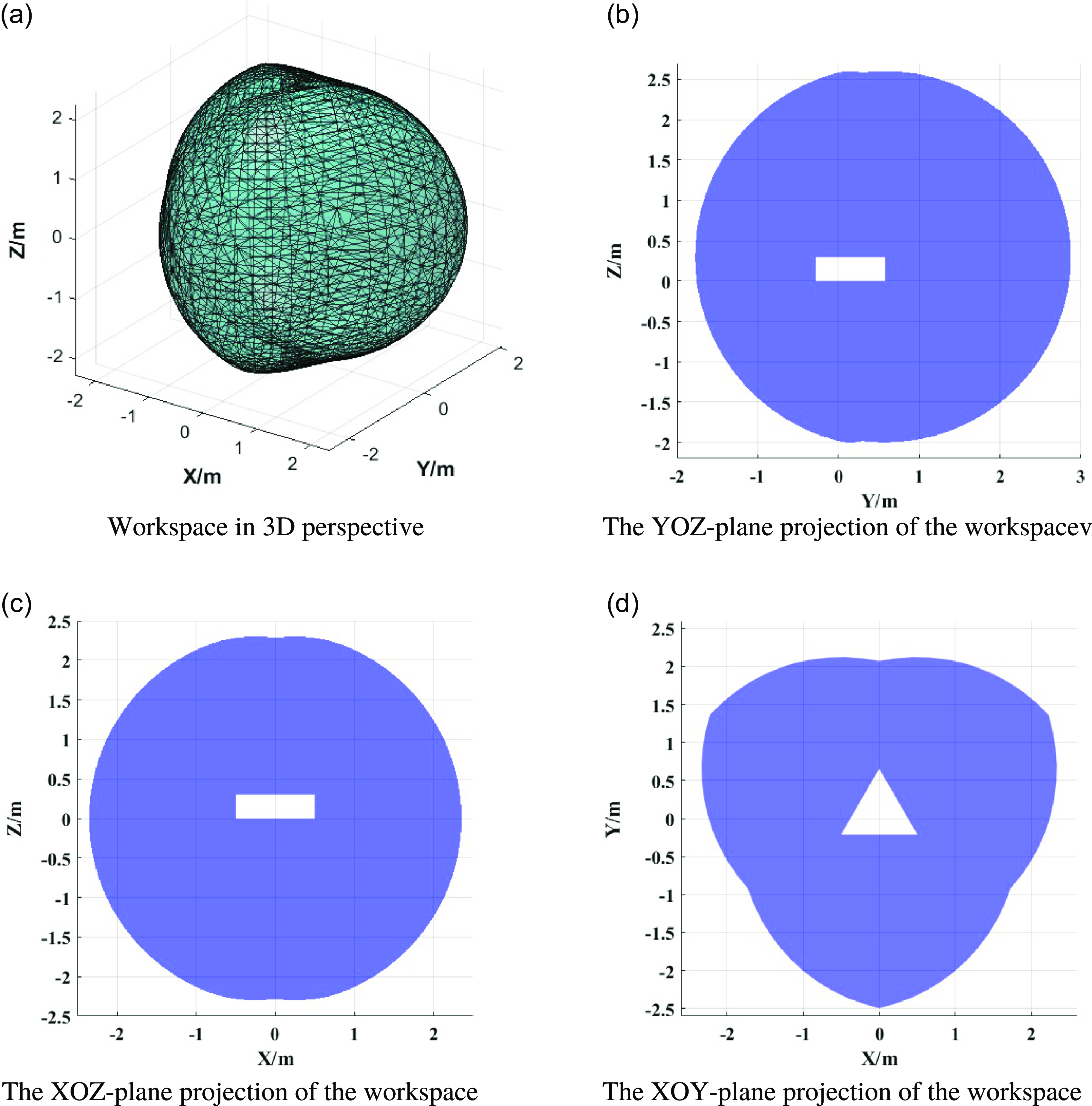
And the collaborative manipulation workspace for every two arms is shown in Figure 5.

Figure 5.

Diagram of collaborative manipulation workspace.

During the transformation process, arm 1 and arm 2 move together until their ends are entirely in contact. Due to the control errors, the velocities of the two ends cannot reach $0$ perfectly. Therefore, assume that there is a residual end velocity of 0.001 m/s along the normal to both ends upon contact. Meanwhile, arm 3 and the base remain stationary before reconfiguration.

Before simulation, some key information about the optimization must be introduced:

• • Optimization objective: Minimization of impulse in non-actuated directions, as shown in (22).

• • Optimization constraint: Self obstacle-avoidance and close-loop constraint.

• • Design variables: Joint angle configuration(lower-level optimization)/contact pose(upper-level optimization).

• • Initial guesses: $\theta _{0}$ (lower-level optimization)/ $x_{0}$ (upper-level. optimization)

• • Simulation platform: Matlab R2023b with Intel i7 8086K at 4.00 GHz, without GPU acceleration or parallel computing.

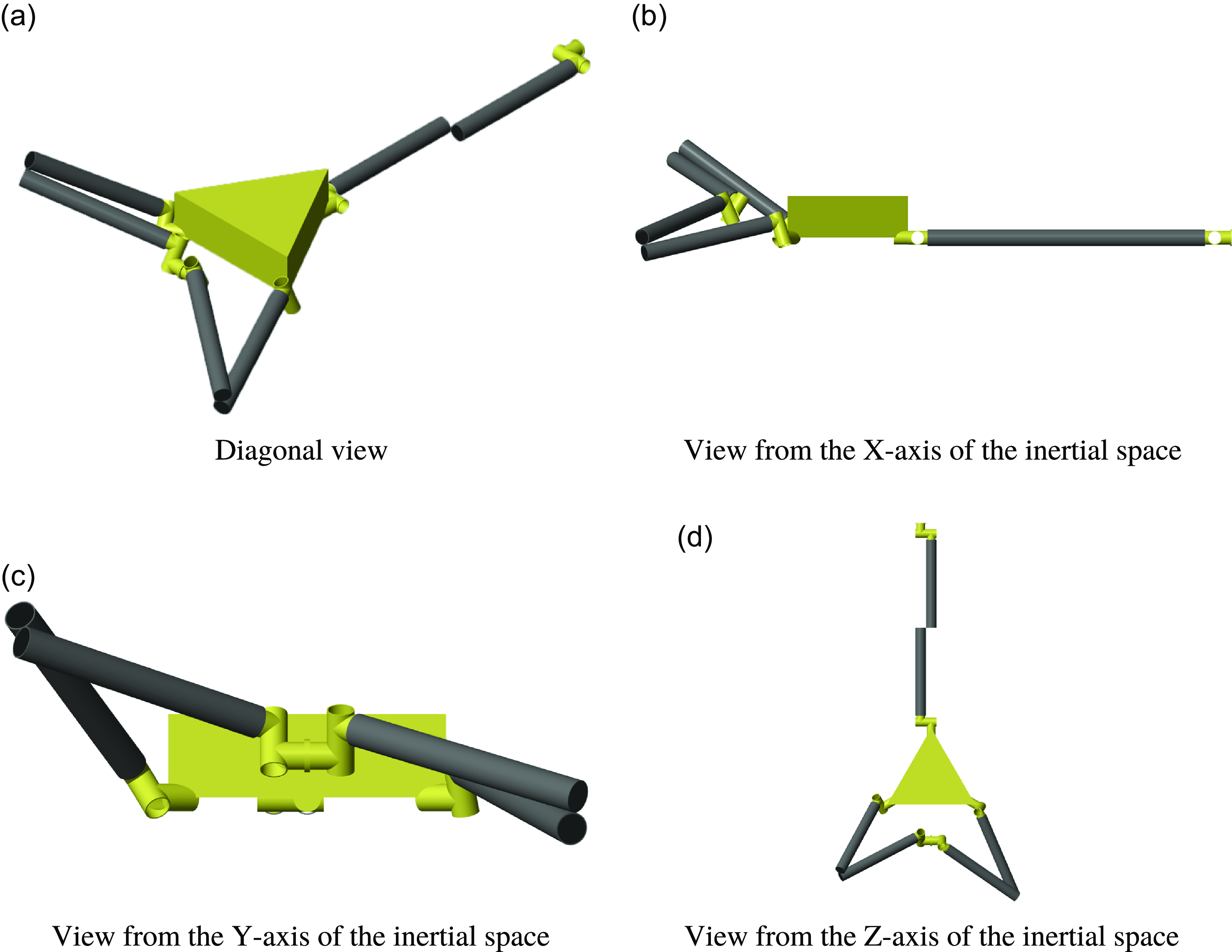
where the $\theta _{0}$ and $x_{0}$ denote the initial guess joint angle configuration and the contact pose, their detailed values are as follows. Based on the initial value above, the impulse before optimization is $0.0031\,{\rm N}\cdot {\rm s}$ . The joint configuration under initial condition is shown in Figure 6.

(32) \begin{equation} \begin{gathered} \theta _{0} =\begin{bmatrix} -0.9945\\ 0.5565\\ -3.0549\\ -2.5366\\ -0.3858\\ 0.7727\\ 2.4558\\ -1.1606\\ -0.6452\\ -0.3217\\ -2.5937\\ 2.7493\\ -0.6720\\ 1.9168 \end{bmatrix} {\rm rad} \\ x_{0} = \bigl [ 0\,\text{m},\ -0.7\,\text{m},\ 0\,\text{m},\ 0\,\text{rad},\ 0\,\text{rad},\ 0\,\text{rad} \bigr ]^T \end{gathered} \end{equation}

Figure 6.

Diagram of space robot at initial contact pose.

First, a lower-level optimization is conducted to verify the effectiveness of lower-level optimization strategy. The solving processes are all run based on MATLAB Optimization Toolbox. The parameters for upper-level optimization with PSO methods are as follows:

• • Particle swarm optimization: Swarm size: 10

• • Max iterations: 100

• • Function Tolerance: 10,000

• • Learning factors $c_{1}$ , $c_{2}$ : 1.49

• • Close-loop coefficient $a_{1}$ , $a_{2}$ : 1.49

• • Repulsion coefficient $k_{r}$ : 5

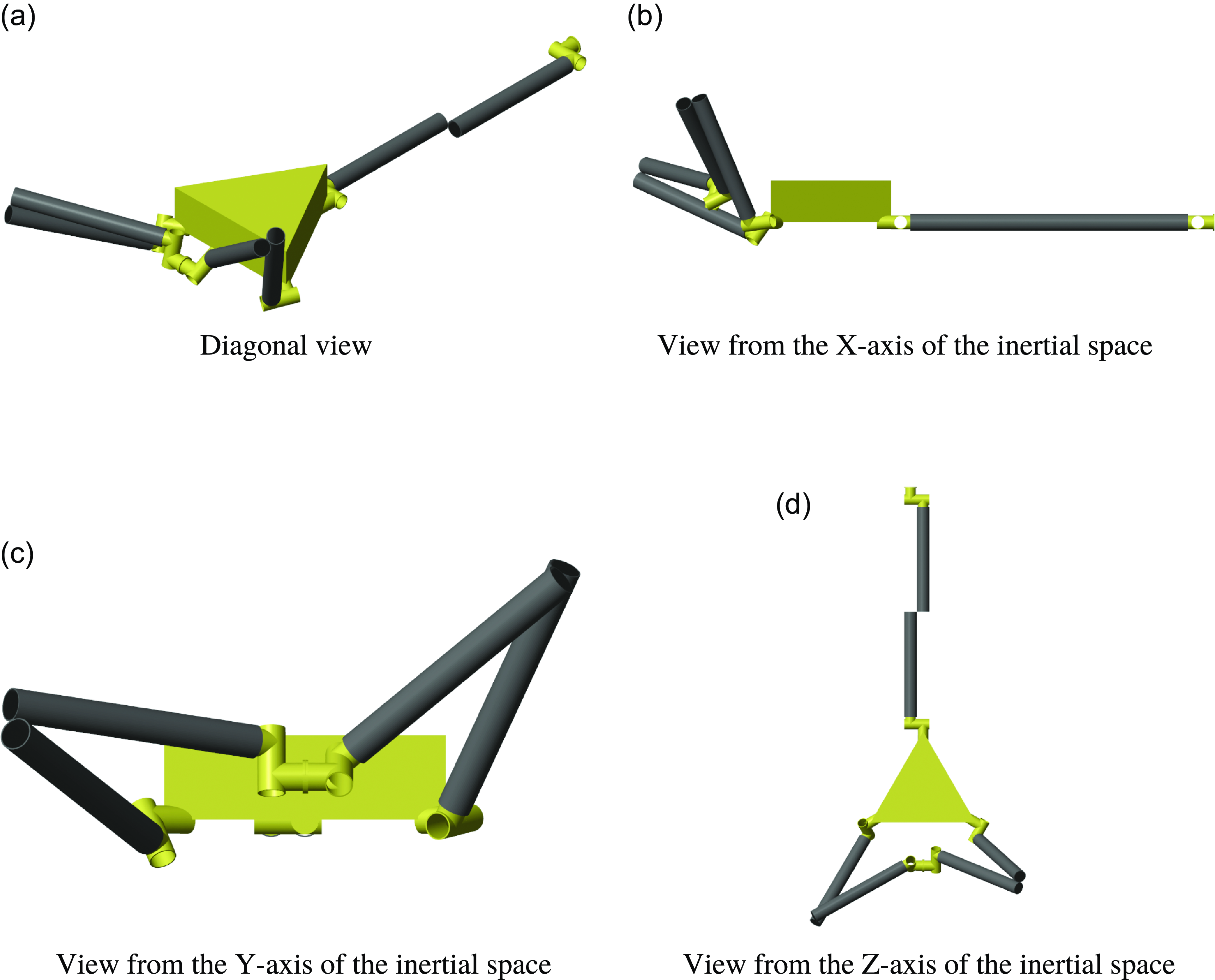
The configuration after optimization is as shown in Figure 7, and the angles is as (33).

Figure 7.

Diagram of space robot after lower-level optimization.

(33) \begin{equation} \begin{aligned} \theta _{1}&=\begin{bmatrix} -1.2994\\ 0.5307\\ 0.2738\\ 2.5763\\ -0.2071\\ -0.6296\\ -0.8879\\ -2.6847\\ -0.7455\\ 2.9956\\ 2.7149\\ 3.5991\\ 1.0266\\ -3.0143 \end{bmatrix} {\rm rad}\\ F_{1}&=0.0022\,{\rm N}\cdot {\rm s} \end{aligned} \end{equation}

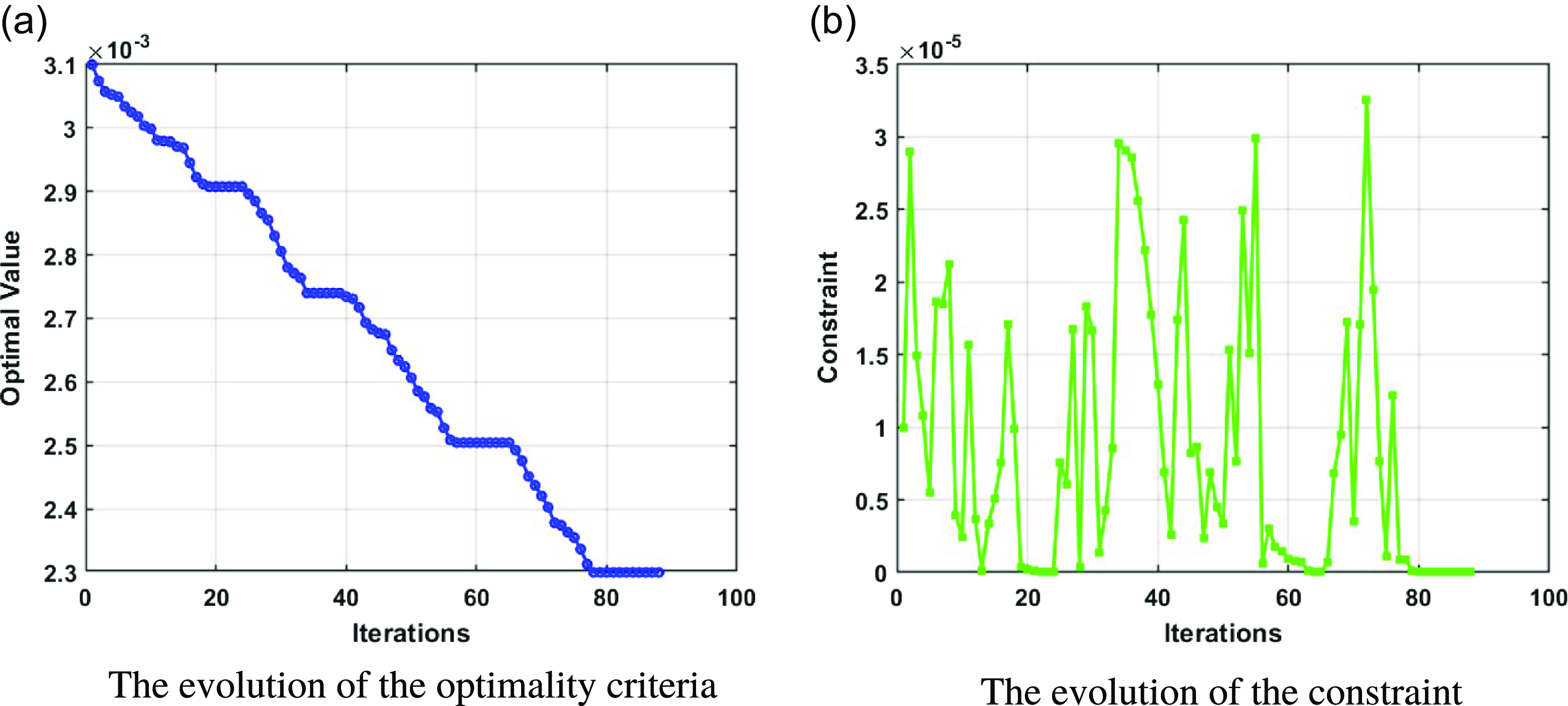
where the $\theta _{1}$ and $F_{1}$ denote the configuration angles after the lower-level optimization and the impulse under this condition. The evolutions of the optimality criteria and constraints are shown in Figure 8.

Figure 8.

The evolutions of lower-level optimization.

From the results, the configuration angles are well optimized and the impulse decreases from $0.0031$ to $0.0022\,{\rm N}\cdot {\rm s}$ . From Figures 6 and 7, the obstacle avoidance constraints and close-loop constraints are well promised. It means that the lower-level optimization strategy is effective for impulse minimization. Thus the bilevel optimization can be further conducted. The computation time for the lower-level optimization is 2142 ${\rm s}$ .

For the bi-level optimization, the model and algorithm are as described in Sections 3 and 4. The solving processes are all run based on MATLAB Optimization Toolbox. The parameters for upper-level optimization with SA methods are as follows:

• • Simulating annealing:

• • Max iterations: 100

• • Function Tolerance: 1e-3

• • Initial temperature: 1.0

• • Cooling function: temperature fast

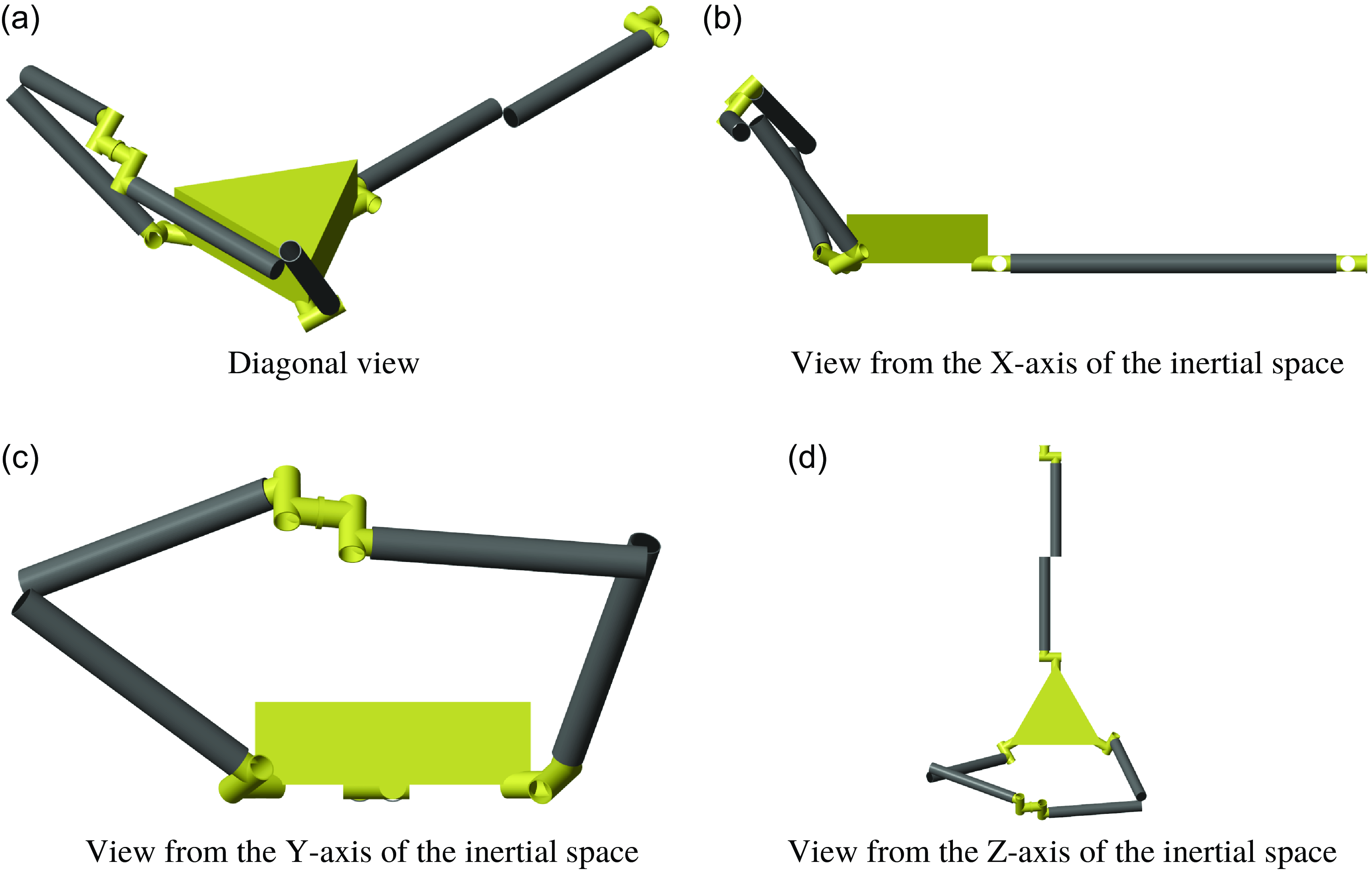
The configuration after bilevel optimization is as shown in Figure 9, and the angles is as (34).

Figure 9.

Diagram of space robot after bilevel optimization.

(34) \begin{equation} \begin{aligned} \theta _{2}&=\begin{bmatrix} 0.0712\\ -0.4193\\ -1.1062\\ 2.1076\\ -0.1311\\ -0.4253\\ -0.4155\\ 2.9746\\ 0.0113\\ 0.5801\\ -1.8031\\ -2.8318\\ -0.9404\\ 0.6106 \end{bmatrix} {\rm rad}\\ F_{2}&=0.0013\,{\rm N}\cdot {\rm s} \end{aligned} \end{equation}

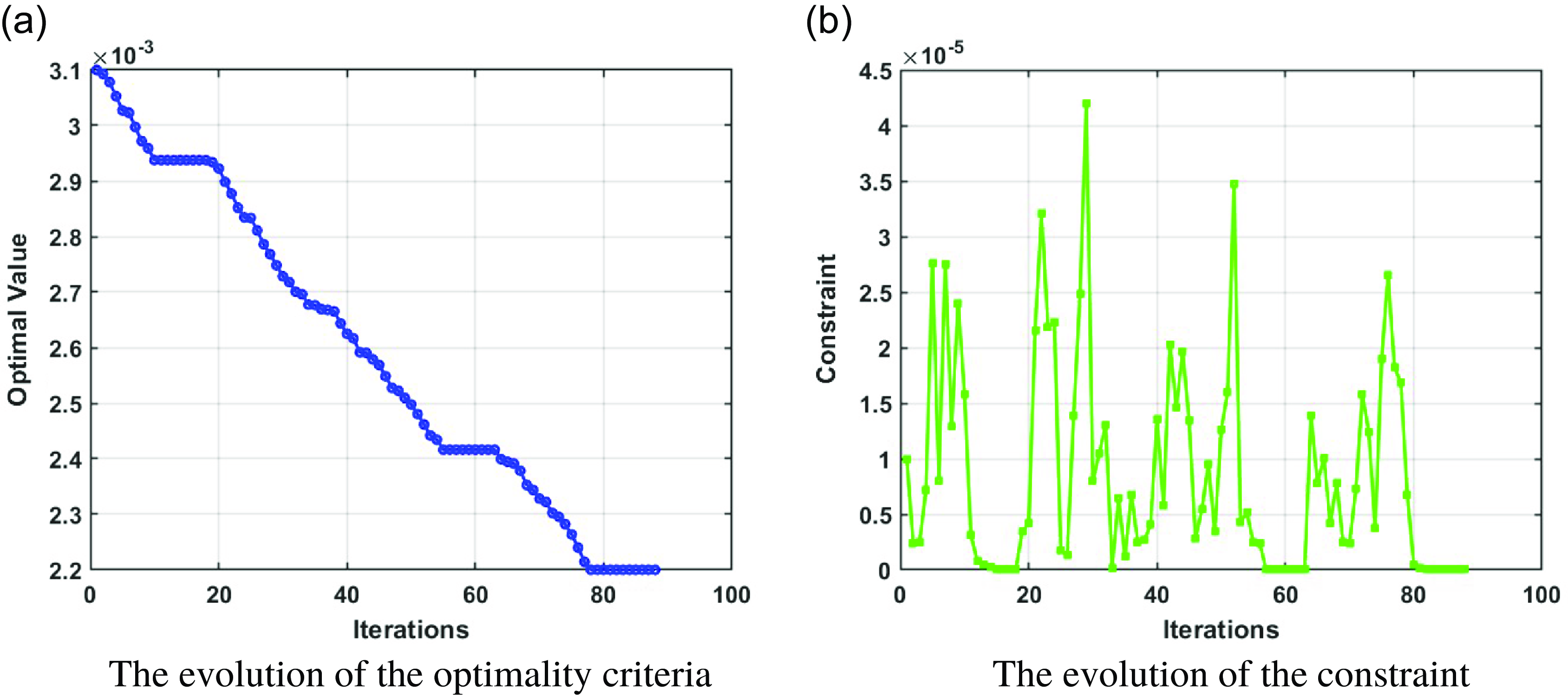
where the $\theta _{2}$ and $F_{2}$ denote the configuration angles after the bilevel optimization and the impulse under this condition. The evolutions of the optimality criteria and constraints are shown in Figure 10.

Figure 10.

The evolutions of bi-level optimization.

After the optimization, the minimum impulse is: 0.0013 ${\rm N} \cdot {\rm s}$ , the contact pose is $\left [-0.265\,{\rm m},\right.\!\!$ $\left.-0.952\,{\rm m},0.835\,{\rm m},0.360\,{\rm rad}, 0.114\,{\rm rad},0.055\,{\rm rad}\right ]^{T}$ , the computation time for the bilevel optimization is 33,784 ${\rm s}$ .

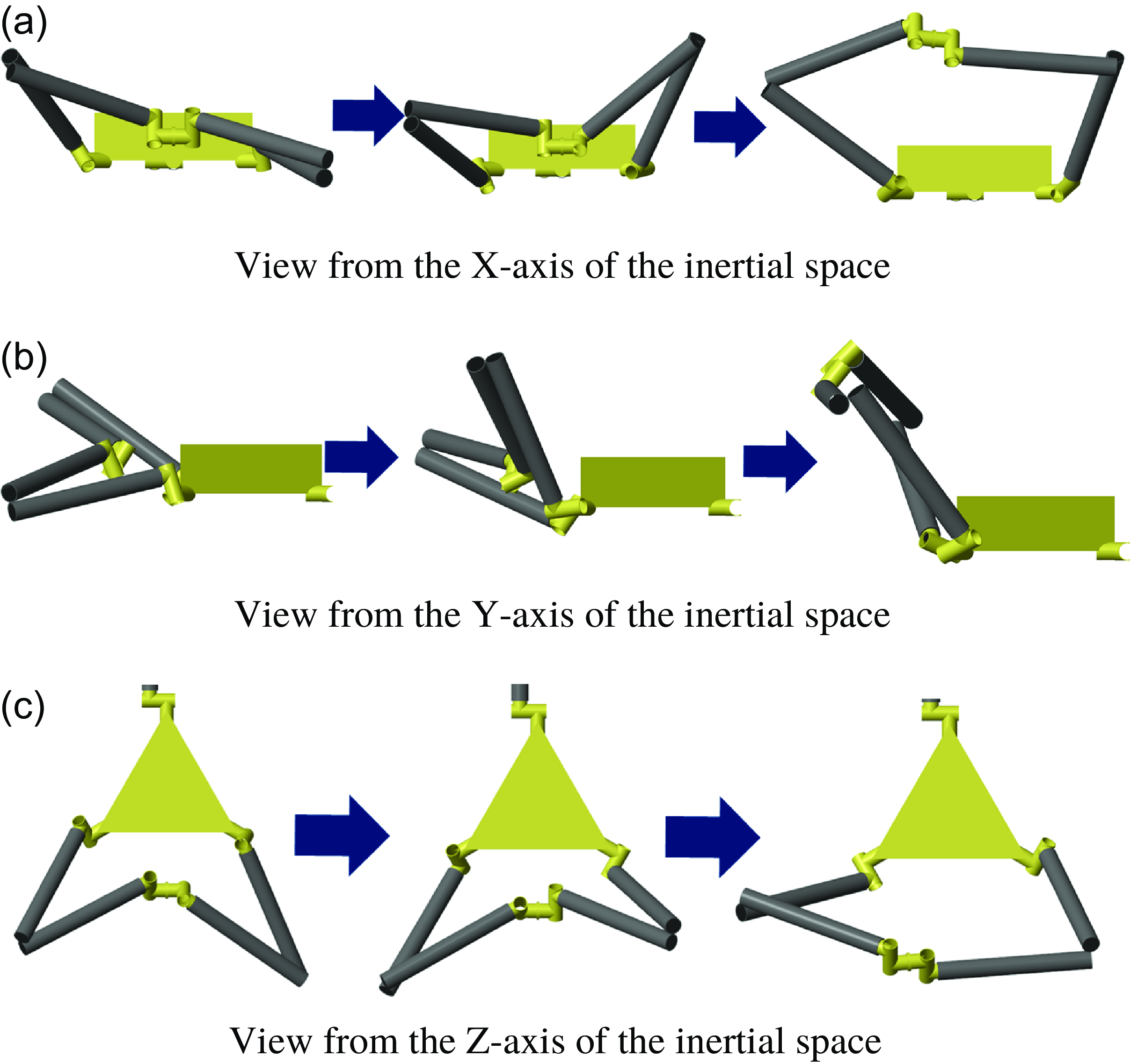
The optimization results demonstrate a reduction in impulse from 0.0031 to 0.0013 ${\rm N} \cdot {\rm s}$ . This suggests that the proposed optimization methods can effectively be employed to design the optimal configuration for this type of space robot. If the total impact that the solid lubricant layer can stand is assumed to be a constant $L_{\max}$ , the maximum number of reconfigurations allowed for the original configuration is $L_{ma}/0.0013$ , and that after optimization is $L_{ma}/0.0031$ . It means that the optimal transformation method can increase the allowable number of reconfigurations for the robotic system by approximately $238\%$ , in other words, extending its operational lifespan by $238\%$ . 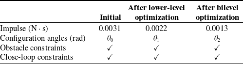In other words, a single robot employing the optimized reconfiguration strategy can accomplish tasks that previously required at least two robots, which significantly reduces the mission costs. The whole optimization results can be summarized in Table II and Figure 11.

Table II.

Optimization results.

Figure 11.

Diagram of configuration changes.