1 Introduction
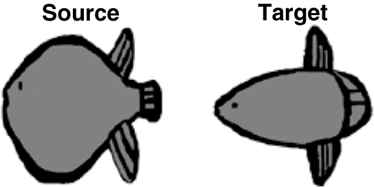
Image registration refers to the process of identifying the optimal transformation that aligns two images, which are commonly referred to as the source and target, so that their appearances closely match. The work of Thompson, in particular his insights into biological forms, serves as a foundational motivation for the development of image registration techniques. In his renowned book On Growth and Form [Reference Thompson47], Thompson introduced the concept of an “isogonal” transformation to describe the relationship between different species. The term “isogonal” is now largely obsolete; the more modern term “conformal” is commonly used in contemporary literature. Conformal transformations are those that preserve local angles [Reference Grigor’ev23, Reference Marsland, McLachlan, Modin and Perlmutter35, Reference Milnor39, Reference Tufail49, Reference Vlasov and Skorokhodov52]. Thompson’s conformal assertions were further explored by Petukhov [Reference Petukhov41], who employed the Möbius group, which is a finite-dimensional subgroup of the group of conformal diffeomorphisms [Reference Tufail49], to assess whether a set of points in the images could be related by Möbius transformations, based on the cross-ratio invariant. Petukhov’s findings suggest that the conformal patterns Thompson observed in his book cannot be disregarded. While Petukhov’s work focused on finite-dimensional groups and sets of points within images, this paper aims to explore conformality within a larger group framework through image registration. This larger group, which is an infinite-dimensional extension of the Möbius group, consists of conformal diffeomorphisms [Reference Marsland, McLachlan, Modin and Perlmutter35, Reference Tufail49].
Significant progress has been made in the field of image registration since 1942, the year in which Thompson’s book was republished. One of the most novel developments is the discovery of diffeomorphic image registration using the method known as large deformation diffeomorphic metric mapping (LDDMM) [Reference Beg, Miller, Trouvé and Younes5, Reference Cao, Miller, Winslow and Younes11, Reference Glaunes, Qiu, Miller and Younes19, Reference Grenander and Miller22, Reference Joshi and Miller28]. A landmark contribution to the field came in 1992, when Brown published the first comprehensive review on image registration [Reference Brown7]. She identified the core components necessary for image registration, which include: (i) a feature space (containing information about the images); (ii) a search space (comprising a set of transformations); (iii) a search strategy (for selecting the optimal transformation); and (iv) a similarity metric (to quantify the difference between the images). Brown suggested only a limited set of finite transformations, which included: (a) affine transformations (for example, shearing, aspect ratio changes and rigid transformations); (b) perspective transformations (that is, transformations that map three-dimensional to two-dimensional); and (c) polynomial transformations (useful when limited information about camera geometry is available) [Reference Marsland, McLachlan and Tufail36, Reference Tufail49]. Although the fundamental steps in image registration have remained largely the same, the range of transformations has evolved significantly. Modern techniques now routinely use diffeomorphisms, which are nonrigid transformations that belong to an infinite-dimensional group. These have become integral to image registration, especially in medical imaging [Reference Grenander and Miller22, Reference Joshi and Miller28, Reference Smith46].
Over the years, numerous methods for image deformation have been developed, spanning diverse fields of mathematics and computer science [Reference Chen12, Reference Dabbour, Habib and Saii14, Reference Frasczek, Cyganek and Wiatr16, Reference Glasbey and Mardia18, Reference Goshtasby20, Reference Grzeszczuk24, Reference Kryjak and Gorgoń30, Reference Saxena and Singh43, Reference Tufail and Gul50, Reference Zitova and Flusser56]. The introduction of diffeomorphic image registration has brought about a novel shift in the field. Diffeomorphisms are smooth functions whose inverses are also smooth [Reference Marsland, McLachlan and Tufail36, Reference Tufail49, Reference Younes55].
The primary objective of this study is to construct a conformal diffeomorphism, denoted by
 $\psi $
, for the purpose of image registration. Over the past 24 years (2001–2024), the use of conformal transformations has been more prevalent than diffeomorphic image registration, as established by our thorough review of bibliometric data on image registration obtained from the SCOPUS repository. Interestingly, researchers have shown a growing interest in using conformal transformations for image registration without incorporating LDDMM, while LDDMM is predominantly used in diffeomorphic image registration.
In this paper, we propose an algorithm to construct conformal diffeomorphisms, thereby facilitating conformal image registration where discretised Cauchy–Riemann equations are used as a penalty term to enforce the conformality condition. Although four distinct penalty terms were discussed in previous work [Reference Marsland, McLachlan and Tufail36, Reference Tufail49], we argue that the first penalty term warrants further investigation, as it is theoretically equivalent to the fourth penalty term. Therefore, this paper focuses on conformal image registration using the first penalty term. All numerical examples presented in this study involve two-dimensional greyscale images [Reference Marsland, McLachlan and Tufail36, Reference Tufail49].
1.1 Image registration using a conformal diffeomorphism
Let
 $\Omega \subset {\mathbb {R}}^2$
be an image domain, and let
 $I_1,I_2\colon \Omega \to \mathbb {R}$
be two greyscale images. We consider
 ${\mathbb {R}}^2$
with the standard complex plane
 $\mathbb {C}$
analogously and write
 $z=x_1+\text {i}x_2$
for
 $(x_1,x_2)\in {\mathbb {R}}^2$
. Let
 $\mathrm {con}(\Omega ,\mathbb {C})$
be the set of maps
 ${\hat {\psi }}$
that obey the following two properties: (i)
 ${\hat {\psi }}(z)$
is complex analytic for all
 $z\in \Omega $
; and (ii)
 ${\hat {\psi }}'(z)\ne 0$
for all
 $z\in \Omega $
. These ensure that
 ${\hat {\psi }}$
is conformal, invertible on its image and has a conformal inverse. We define the objective function in equation (1.1) as
 $$ \begin{align} E(\hat{\psi})=\int_{\Omega}{((I_{1}\circ{\hat{\psi}}^{-1})(x)-I_2(x))^2}\,dx_1\, dx_2, \end{align} $$
where
 $x=(x_1, x_2)^T$
and
 $\hat {\psi }\in \mathrm {con}(\Omega ,\mathbb {C})$
. A process in which we find a
 $\hat {\psi }$
that minimizes
 $E({\hat {\psi }})$
over
 $\hat {\psi }\in \mathrm {con}(\Omega ,\mathbb {C})$
is called a conformal image registration.
The challenges encountered in image registration also arise in the context discussed here. Two key difficulties are: (i) the domain of
 $I_1\circ {\hat {\psi }}^{-1}$
is
 ${\hat {\psi }}(\Omega )$
, rather than
 $\Omega $
, that is, the domains of the target image and the transformed source image do not coincide; and (ii) the selection of an appropriate optimization algorithm. These issues are well established in the literature [Reference McLachlan and Marsland38, Reference Modersitzki40, Reference Younes55].
A novel complication in the context of infinite-dimensional image registration (that is, registration involving infinite-dimensional groups such as the full set of diffeomorphisms or the conformal group, as discussed in this paper) is the representation of diffeomorphisms. For diffeomorphic registration, this issue has been addressed in various ways [Reference Arsigny, Commowick, Ayache and Pennec3, Reference Beg, Miller, Trouvé and Younes5, Reference Hsiao, Hsieh, Chen, Gong, Luo and Liao26, Reference Marsland and McLachlan34, Reference Marsland and Twining37], and these representations may, in turn, influence the optimization process. In this study, however, we specifically focus on the representation of conformal maps.
Equation (1.1) provides a general formulation of an objective function pertinent to image registration. However, our focus in this work is on conformal image registration. Consequently, the task of minimizing
 $E({\hat {\psi }})$
can be framed as a constrained optimization problem, where
 ${\hat {\psi }}$
in equation (1.1) represents conformal diffeomorphisms. To address this, we introduce a penalty term that enforces the conformality of the diffeomorphism. Thus, instead of using the objective function presented in equation (1.1), we adopt the modified objective function
 $$ \begin{align} E(\psi)=\int_{\Omega}{\{(I_{1}\circ \psi^{-1})(x)-I_2(x)\}^2}dx_1\, dx_2+\lambda\int_{\Omega} P(y)^2\,dy_1\, dy_2. \end{align} $$
Here,
 $P(y), y=(y_1,y_2)$
is a penalty term that vanishes if and only if
 $\psi $
is a conformal diffeomorphism, that is, if and only if
 $\psi $
satisfies the Cauchy–Riemann equations [Reference Greenfield21, Reference Wells53] at the points y and has nonzero derivative.
The second term in equation (1.2) is commonly referred to as the regularization term in the literature [Reference Bouhamidi and Jbilou6, Reference Burger, Modersitzki and Ruthotto8, Reference Calvetti, Morigi, Reichel and Sgallari10, Reference Tustison and Avants51, Reference Ying, Xu and Liang54]. In the context of image registration, the inclusion of this regularization term alongside the conventional registration formulation is typically termed Tikhonov regularization [Reference Tikhonov48]. The first term in equation (1.2) measures the degree of alignment between the transformed image and the target, thereby representing a quantification of data fidelity or, alternatively, the degree of misalignment. By contrast, the regularization term imposes constraints on the structural properties of the transformation, ensuring that it adheres to specific, predefined conditions. In this case, the transformation is constrained to be conformal, which means that it preserves angles while allowing for local variations in scale. This regularization is essential for maintaining both mathematical stability and physical plausibility, especially when the data are contaminated by noise or when the registration problem is ill posed. The regularization parameter, denoted by
 $\lambda $
in equation (1.2), governs the trade-off between image matching and the corresponding constraints imposed during the optimization process (in this case, conformality). This approach to regularization has been widely applied in various fields, with the specific choice of constraints tailored to the requirements of each domain. For instance, Stuart Crozier and his research group at the University of Queensland have employed different regularization parameters in inverse electrocardiography models [Reference Shou, Jiang, Xia, Wei, Liu and Crozier45], while Tikhonov regularization has been applied to noise reduction, where the regularization parameters function as Lagrange multipliers [Reference Jackson, Brideson, Forbes and Crozier27]. Similar approaches have been explored in other studies [Reference Liu, Wang, Sun, Chandra, Crozier and Liu33, Reference Poole, Lopez and Crozier42, Reference Shan, Li, Tang, Ma, Liu and Crozier44].
Equation (1.2) is continuous; however, for practical numerical computation, a discretized form of the objective function is required. Discretization is essential for the implementation of the registration algorithm on a computational grid. The discretized formulation is examined in greater detail in the following section, where the steps involved in numerical evaluation and optimization are outlined.
The remainder of this paper is organized as follows. We define the discretized form of the objective function in Section 2. Section 3 is dedicated to the formulation of the penalty term, which is based on the concept of a “discrete conformal map”, and we test it using Algorithm 1. The implementation of Algorithm 1 is presented in Section 4. Finally, the conclusions of the research are discussed in Section 5.
2 Control point method
In this section, we define our method for conformal image registration in a similar manner to how it was defined by Marsland et al. [Reference Marsland, McLachlan and Tufail36] (see [Reference Tufail49, Ch. 3]. First we present a discrete form for equation (1.2). We represent our discrete domain by D, which indicates the location of pixels. Typically, these are arranged in an
 $N\times N$
square in
 $[-0.5,0.5]^2$
leading to
 $N^2$
pixels at locations
 $x_{ij}$
. This strategy remains the same for all the numerical examples that are presented in Section 4. In the control points method, the map
 $\psi $
is represented by the values of
 $\psi ^{-1}$
on a much coarser grid than that of the discrete image domain D. Thus, we first choose
 $n^2$
grid points
 ${\hat {x}}_{ij}$
(
 $i,j=1,\dots ,n$
) from the discrete domain D, where
 $n\ll N$
, that are configured in an
 $n\times n$
grid. We then transform these chosen points under
 $\psi ^{-1}$
to generate another set of points of the same size. We define two sets of points: the set of chosen points
 ${\hat {x}}_{ij}=\{{\hat {x}}_{11},{\hat {x}}_{12},\dots ,{\hat {x}}_{nn}\}$
, and the set of transformed points
 ${\hat {y}}_{ij}=\{{\hat {y}}_{11},{\hat {y}}_{12},\dots ,{\hat {y}}_{nn}\}$
such that
 ${\hat {y}}_{ij}=\psi ^{-1}({\hat {x}}_{ij})$
. Here,
 ${\hat {x}}_{ij}\in D$
and
 ${\hat {y}}_{ij}\in {\mathbb {R}}^2$
. The variables
 ${\hat {y}}_{ij}$
, which determine the map
 $\psi $
, are the dependent variables whose values is determined during the optimization process. Larger values of n make the optimization process much more expensive (in computation sense). The remaining values of
 $\psi ^{-1}$
that are needed to transform the source image, namely,
 $\psi ^{-1}(x_{ij}$
), are determined by bilinear interpolation from the known values
 $\psi ^{-1}({\hat {x}}_{ij})$
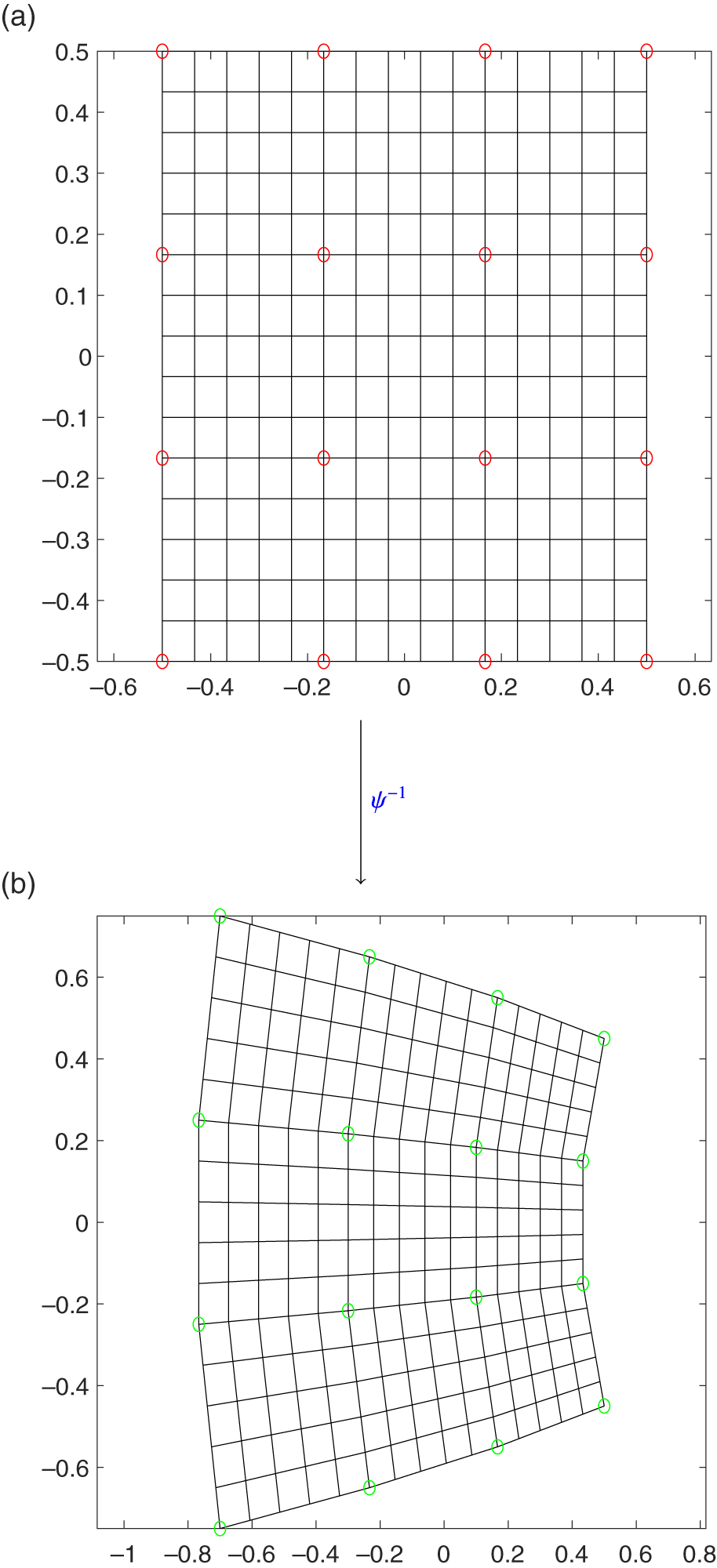
. The illustration of this approach with
 $n=4$
, that is, 16 control points, and with
 $N=16$
, that is, 256 grid points, is given in Figure 1.
(a) The red circles represent
 $n=4$
selected control points from the discrete domain D over
 $N^2$
grid points. (b) The transformed control points under
 $\psi ^{-1}$
are represented by green circles. Matlab-based bilinear interpolation was applied to generate the rest of the grid points between these green circles, that is,
 $N^2=256$
.

The discrete form of equation (1.2) is now defined as
 $$ \begin{align} E(\psi)=\sum_{i=1}^{N}\sum_{j=1}^{N}((I_{1}\circ\psi^{-1})({\hat{x}}_{ij})-I_{2}({\hat{x}}_{ij}))^2+\lambda \sum_{i=1}^{n}\sum_{j=1}^{n} P({\hat{y}}_{ij})^2. \end{align} $$
Equation (2.1) represents the general form of optimization function that is used in this paper. It has two parts: the first part measures how well registered the images are, whereas the second part contains a penalty term P related to the conformality of
 $\psi $
. The two terms are balanced by a regularization parameter
 $\lambda $
. This regularization term
 $\lambda $
supervizes the trade-off between the quality of the registration and the conformality of
 $\psi $
. In this paper, our penalty term is based on the discrete Cauchy–Riemann equations. Here, we have two continuation parameters n and
 $\lambda $
. If we set
 $\lambda =0$
, then the optimization problem reduces to a general problem of image registration and conformality would be dropped out. For very large value of
 $\lambda $
, constraint would be satisfied but image matching would be compromised. Thus, we settled on (through several numerical experiments, not reported here)
 $\lambda =(1/10)N\approx 10$
,
 $N=100$
in all the experiments. The choice of n is another task and we opted for a continuation method in a simpler form. This strategy is chosen from a lecture of Keller [Reference Keller29], who is considered to be the pioneer of this technique. In all of our numerical experiments, started with
 $n=4$
, that is, 16 control points, and optimized (minimization) the objective function in equation (2.1) for
 $\lambda =10$
, using the output of this optimization as the input for
 $n=8$
, that is, 64 control points. We initialized the values for the new points by using Matlab-based bilinear interpolation (interp2, see [Reference Hajovsky, Filipova, Pies and Ozana25] for further details) from the previous solution, that is, the solution corresponding to
 $n=4$
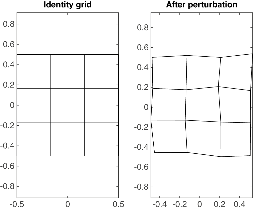
. This whole idea is summarized in Algorithm 1. Our optimization was based on the gradient descent approach, and we used lsqnonlin [Reference Burgos, Hizon and Sison9] from the optimization tool box in Matlab. In all of the experiments, we used small perturbation by adding a uniform pseudorandom number in the interval [0, 0.05] in the control points. The reason for this perturbation was that we did not want our optimizer to be stuck on identity. Comparison of the identity and perturbed grids can be seen in Figure 2.

(a) The original set of control points. (b) The same points with a small perturbation added to each point independently in x and y.

Remark 2.1. It is important to note that the conformal maps generated by this algorithm were derived entirely through numerical methods, rather than relying on traditional transformations such as rotation or scaling. These maps are constructed from equation (2.1), where the first term addresses the image matching, while the second term represents the penalty function (based on the Cauchy–Riemann equations, as shown in equation (3.5) below) that enforces the conformality condition.
3 Derivation of the penalty term
In this section, we derive our penalty that is used in all of the numerical experiments. This penalty term is based on the Cauchy–Riemann equations. Recall the Cauchy–Riemann equations as follows.
If
 $$ \begin{align*} \psi(x, y) = u(x, y) + \text{i}v(x, y)\end{align*} $$
is a conformal map, then
 $$ \begin{align} \frac{\partial u}{\partial x}=\frac{\partial v}{\partial y}, \quad \frac{\partial u}{\partial y}=-\frac{\partial v}{\partial x}. \end{align} $$
Equation (3.1) represents the standard form of the Cauchy–Riemann equations for continuous variables. We can also express them in complex notation. Partial derivatives of
 $\psi $
are defined as
 $$ \begin{align} \frac{\partial \psi}{\partial x}=\frac{\partial u}{\partial x}+\text{i}\frac{\partial v}{\partial x}\end{align} $$
and
 $$ \begin{align} \frac{\partial \psi}{\partial y}=\frac{\partial u}{\partial y}+\text{i}\frac{\partial v}{\partial y}.\end{align} $$
Equations (3.2) and (3.3) yield
 $$ \begin{align} \frac{\partial \psi}{\partial x}+\text{i}\frac{\partial \psi}{\partial y}&=\frac{\partial u}{\partial x}+\text{i}\frac{\partial v}{\partial x}+\text{i}\bigg(\frac{\partial u}{\partial y}+\text{i}\frac{\partial v}{\partial y}\bigg)\nonumber\\&=\frac{\partial u}{\partial x}+\text{i}\frac{\partial v}{\partial x}+\text{i}\frac{\partial u}{\partial y}-\frac{\partial v}{\partial y}\nonumber\\&=\frac{\partial v}{\partial y}+\text{i}\frac{\partial v}{\partial x}+\text{i}\bigg(-\frac{\partial v}{\partial x}\bigg)-\frac{\partial v}{\partial y}\quad{\text{(from equation (3.1))}}\nonumber\\&=0\nonumber\\\implies\kern-4pt \frac{\partial \psi}{\partial x}&=-\text{i}\frac{\partial \psi}{\partial y}. \end{align} $$
Equation (3.4) serves as a complex form of the Cauchy–Riemann equations for continuous variables. For numerical computation, we discretize our domain, and thus we need a discrete form of the Cauchy–Riemann equations. We now present the discrete form of the Cauchy-Riemann equations. These equations are defined by finite differences at each of the
 $n^2$
control points. First, we compute the numerical gradient and then determine the Cauchy–Riemann equations. Note that we identify
 ${\mathbb {R}}^2$
with the complex plane
 $\mathbb {C}$
as needed.
We calculate the gradient of
 ${\hat {y}}_{ij}$
using central differences at the interior points
 $$ \begin{align*} ({{\Delta}_x} {\hat{y}})_{i,j}= ({\hat{y}}_{i+1,j} - {\hat{y}}_{i-1,j})/2 \quad \mbox{for all }{i=2,3,\ldots,n-1,}\\ ({{\Delta}_y} {\hat{y}})_{i,j}= ({\hat{y}}_{i,j+1} - {\hat{y}}_{i,j-1})/2 \quad \mbox{for all }{j=2,3, \ldots, n-1,} \end{align*} $$
and one-sided differences at edge points
 $$ \begin{align*} ({{\Delta}_x}{\hat{y}})_{1,j}={\hat{y}}_{2,j}-{\hat{y}}_{1,j},\quad ({{\Delta}_x}{\hat{y}})_{n,j}={\hat{y}}_{n,j}-{\hat{y}}_{n-1,j},\nonumber\\ ({{\Delta}_y}{\hat{y}})_{i,1}={\hat{y}}_{i,2}-{\hat{y}}_{i,1},\quad ({{\Delta}_y}{\hat{y}})_{i,n}={\hat{y}}_{i,n-1}-{\hat{y}}_{i,n}. \nonumber \end{align*} $$
Identifying
 ${\hat {y}}$
with
 $\psi $
, the discrete form of the Cauchy–Riemann equations that we use is
 $$ \begin{align*} {{\Delta}_x} {\hat{y}}_{ij}=-\text{i}{{\Delta}_y} {\hat{y}}_{ij} \quad \mbox{for all }i,j=1,\dots,n .\end{align*} $$
Note that we are using here the fact that the reference grid of control points,
 ${\hat {x}}_{ij}$
, is a uniform square grid, as we use such a grid in all our experiments. The mesh size of this grid has been effectively absorbed into the parameter
 $\lambda $
. This discrete form of the Cauchy–Riemann equation is used to define the penalty term as
 $$ \begin{align} P_1({\hat{y}}_{ij})=|({{\Delta}_x} {\hat{y}}_{ij}+\text{i} {{\Delta}_y} {\hat{y}}_{ij})|.\end{align} $$
Equation (3.5) serves as the penalty term throughout the paper. We found in our numerical experiments (not reported in this paper) that when
 $\lambda \to \infty $
,
 $\|P_{1}({\hat {y}})\|\to 0$
, and that the discrete maps produced in this way were always rigid transformations, that is, Euclidean similarities [Reference Ashburner and Friston4, Reference Elmore and Richman15].
4 Experiments
In this section, we present the implementation of Algorithm 1 through four distinct examples. We begin by selecting a set of smooth images for registration, as these tend to be easier to register. Subsequently, we introduce three examples of nonsmooth images. For each of these nonsmooth examples (Examples 4.2, 4.3 and 4.4), we apply a smoothing process using a Gaussian kernel to transform the source and target images into smooth versions (see [Reference Tufail49, Section 3.1.1]). Algorithm 1 is first applied to the smoothed images, after which a final registration step is performed using the original unsmoothed images. This approach allows the preliminary registration steps with the smoothed images to serve as a means of obtaining a reliable initial guess for the final registration.
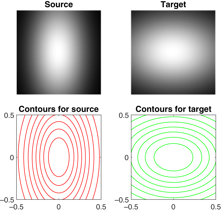
Example 4.1. In this introductory example, we select a set of smooth Gaussian images, which are not a priori assumed to be conformally related. These Gaussian images, along with their corresponding contour plots, are presented in Figure 3.
The source and target images for Example 4.1. The source is
 $e^{-7x^{2}- 2y^{2}}$
and the target is
 $e^{-2x^{2} -4y^{2}}$
. The corresponding contour plots can be seen in the second row.

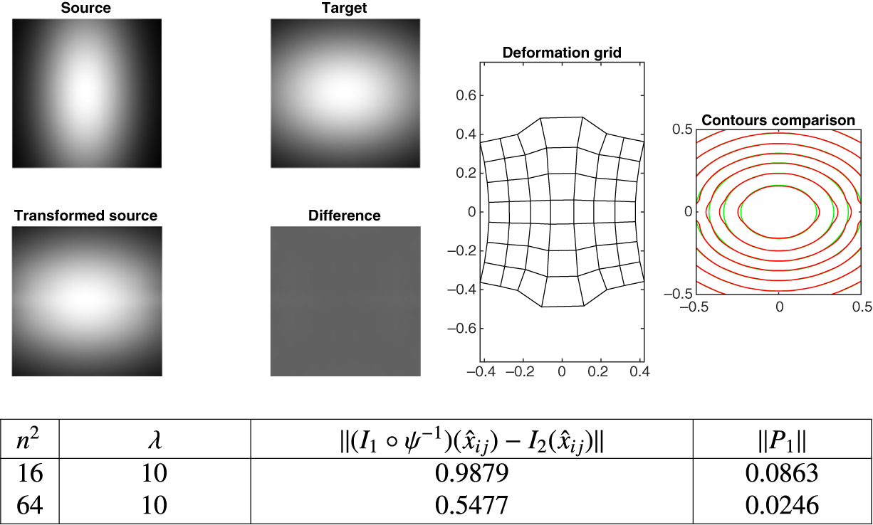
According to the Riemann mapping theorem (see [Reference Frederick and Schwartz17, page 55], [Reference Ahlfors2, pages 221–224] and [Reference Leonhardt31], there is a conformal map that takes any one contour of the source to the same contour of the target. This map is unique up to an element of the (three-dimensional) disc-preserving Möbius group. Thus, in general, there is not enough freedom left to match any of the other contours. The conformal map that transforms a circle into an ellipseFootnote 1 maps concentric circles to confocal ellipses. The literature suggests several possible conformal transformations, including translation, scaling, rotation, the Zhukovskii transformation, truncated Taylor series and others [Reference Abbott and Von Doenhoff1, Reference Conway13, Reference Lin, Wu, Bloom, Cox, Miller and Lui32]. However, it is important to note that, in this example and throughout the manuscript, the conformal maps are generated using numerical methods based solely on equation (2.1) and Algorithm (1). Although we hypothesize that the source and target are not conformally related—due to their lack of confocality—the primary goal of conformal image registration is to identify the optimal conformal map that maximizes the alignment between the transformed source and the target. The implementation of Algorithm 1 in this context is illustrated in Figure 4. The results clearly demonstrate that a successful conformal registration has been achieved.

Following the successful conformal image registration for a pair of smooth images, we now present three examples involving nonsmooth images, progressing from easier to more challenging cases as outlined below.
-
(1) Synthetic data example: this is a nonsmooth source image, with the target generated from the source by a known conformal map.
-
(2) Nonsynthetic data example: this is a nonsmooth source image and an independent, yet nearly conformally related, target.
-
(3) Nonsynthetic data example with unrelated images: this is a nonsmooth source and target that are not known to be conformally related.
In this progression, we demonstrate varying levels of difficulty in conformal registration, from controlled synthetic data to more complex scenarios.
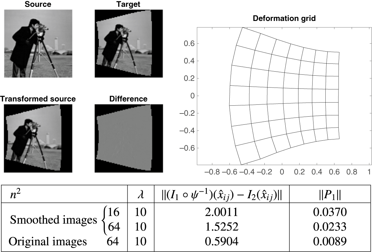
Example 4.2. Figure 5 presents two examples of the standard “cameraman” image. This example uses synthetic data, where the target image is generated from the source through the known conformal transformation
 $\psi ^{-1}(z) = 0.1 + 1.2z -0.3z^2+0.2z^3$
.
The images for Example 4.2. The source
 $I_1$
is a standard reference image; the target is
 $I_2(z) = I_{1}(0.1 + 1.2z -0.3z^2+0.2z^3)$
, that is,
 $I_2$
is generated with the known conformal transformation.

As described in Section 4 above, we first perform the registration of smooth images for the given pair of nonsmooth images (for
 $n=4$
and
 $n=8$
) The optimized result from this step is then used as an initial estimate for the registration of the original source and target images at
 $n=8$
. The result of this registration process is shown in Figure 6.
The results of the first attempt at registration for Example 4.2. An excellent registration, along with a smooth conformal grid, is obtained.

The algorithm achieved an excellent conformal registration, with a smooth grid. The only remaining errors are attributable to the representation of the quadratic
 $\psi ^{-1}(z)$
on the grid and the form of the discrete Cauchy–Riemann equations employed. The root-mean-square error is 0.0059 per pixel (relative to image values, which range from [0,1]), and all the primary features of the images have been successfully aligned.
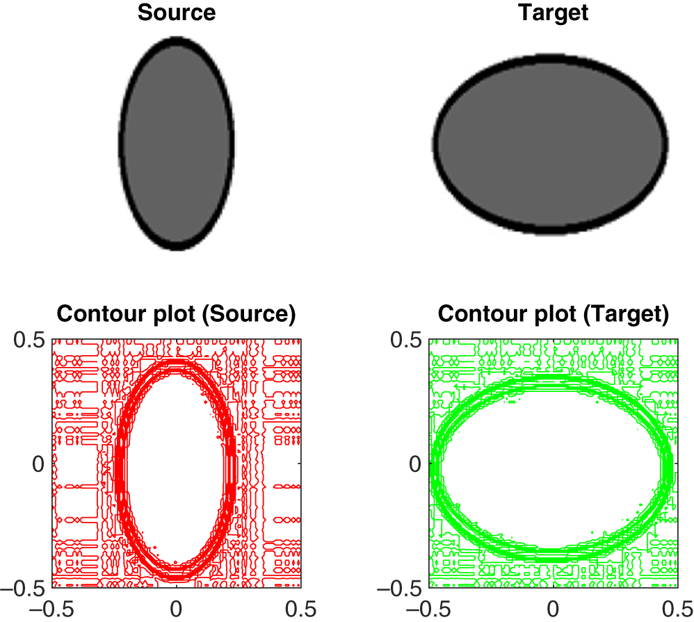
Example 4.3. We now present a conformal image registration for nonsmooth images, where the source and target are independent but known to be (nearly) conformally related. These images are shown in Figure 7.
The two nonsmooth images of ellipses for Example 4.3 are given along with their respective contour plots in the second row.

The source and target images consist of filled ellipses with varying aspect ratios. Notable, albeit subtle, textural differences between the two images are visible in the background. These differences arise from interpolation artefacts, which result from mapping the images onto a
 $100 \times 100$
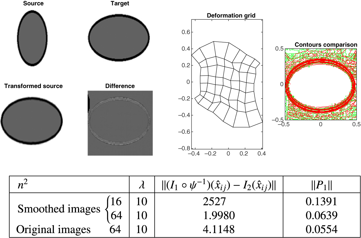
pixel grid. According to the Riemann mapping theorem, there exists a conformal map that transforms the interior of one ellipse to the interior of another. However, this map exhibits singularities outside the ellipses, which presents a potential challenge for this example. The black borders in the images encourage the algorithm to closely align the boundaries, but we hypothesize that a conformal map exists that can nearly align the images. The results of the conformal image registration process are presented in Figure 8.

Through a series of extensive numerical experiments (details are omitted here for brevity), we observed that varying the value of
 $\lambda $
had minimal impact on the results for smooth images. By contrast, for nonsmooth images, particularly those derived from nonsynthetic data, the effect of
 $\lambda $
was more significant. Image registration for nonsmooth images is inherently challenging, and, consequently, we intend to further investigate this behaviour by examining both the current and subsequent examples across a range of
 $\lambda $
values.
Conformal image registration aims to find an optimal inverse map
 $\psi ^{-1}$
that achieves a reasonable match, or at least minimizes the mismatch, between the transformed source and the target, while maintaining smooth, conformal grid structures. Initial results were perplexing, and we were uncertain about selecting an appropriate value for
 $\lambda $
. Rather than testing individual values, we chose to directly solve the minimization problem at
 $\lambda = 10$
(for smooth images first, followed by nonsmooth ones). We then employed parameter continuation by adjusting
 $\lambda $
in a constant ratio for nonsmooth images. The results of these experiments are shown in Figures 9 and 10. In the first set of experiments, where
 $\lambda \in [6.75, 10]$
, visually good registration was achieved, with registration errors between 4.04 and 4.11. The second set of experiments also yielded satisfactory registration for all values of
 $\lambda $
, accompanied by smooth conformal grids. In this case, all grids (except those corresponding to very small or very large values of
 $\lambda $
, that is,
 $\lambda \geq 500$
) exhibited the “square-to-square” property.
(a) Series of transformed sources as
 $\lambda $
is decreasing (smaller
 $\lambda $
, that is, less conformality enforced) geometrically. (b) The corresponding grids.

(a) Series of transformed sources are given when
 $\lambda $
is increasing (larger
 $\lambda $
, that is, more conformality enforced) geometrically. (b) Series of grids are presented corresponding to
 $\lambda $
.

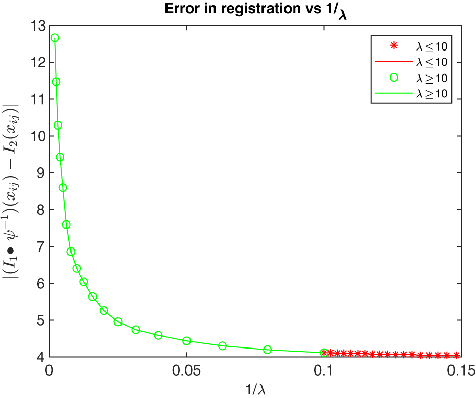
Alternatively, the value of
 $\lambda $
can be determined using the L-curve method, as illustrated in Figure 11. This plot, characterized by its distinct “L” shape, clearly shows that values of
 $\lambda \leq 10$
result in nearly identical errors. The L-curve further suggests that the optimal range for
 $\lambda $
in this example lies between 20 and 80.
A combined L-curve for two geometric series (increasing and decreasing) with a common parameter
 $\lambda $
is shown in Example 4.3. Here,
 $\lambda =10$
is the common value for both of the series. This curve illustrates the relationship between the registration error and
 $1/\lambda $
. For
 $\lambda \leq 10$
, the error remains approximately the same.

The images for Example 4.4.

The results of registration for Example 4.4 at
 $\lambda =10$
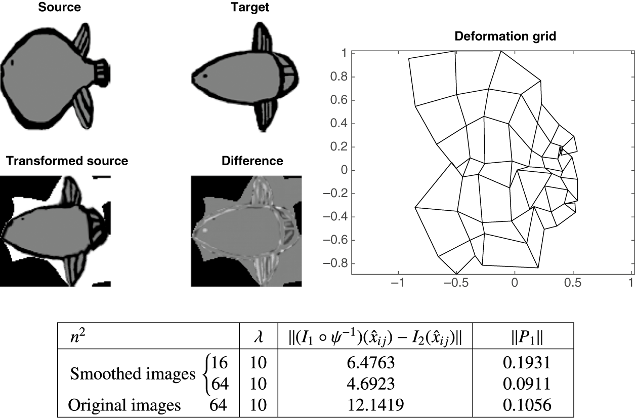
. The transformed source is perfectly aligned with the target. However, the grid is not smooth, which means that the task of conformal diffeomorphisms has not been achieved.

(a) Series of transformed source (when
 $\lambda $
is decreasing geometrically). (b) Corresponding grids for the series.

(a) Series of transformed source (when
 $\lambda $
is increasing geometrically). (b) Corresponding grids for the series.

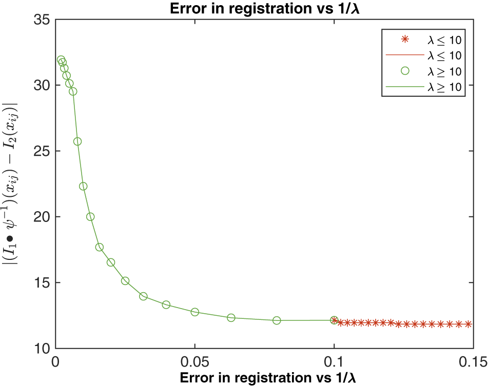
L-shaped curve for the error of registration in Example 4.4. The red line and * indicate the corresponding errors when
 $\lambda $
is decreasing. The green line and “o” represent the errors in registration when
 $\lambda $
is increasing geometrically.

Example 4.4. In this final example, we investigate the registration of two nonsmooth images that are hypothesized to be related by a conformal transformation. Thompson, in his seminal work [Reference Thompson47], suggested that a particular pair of his fish images (see Figure 12) could be linked through an isogonal (conformal) transformation. For the current experiment, the original images were digitized from Thompson’s On Growth and Form [Reference Thompson47], with the contours of the fish delineated using a black marker. Any extraneous grid lines were digitally removed, and the hand-drawn images were scanned. The interiors of the fish were filled with a grey colour using Microsoft Paint, a step undertaken to facilitate the optimization process. The images were then resized to a
 $100 \times 100$
pixel grid using MATLAB’s imresize function, which employs bi-cubic interpolation. The addition of grey shading inside the fish was specifically intended to aid in the image registration optimization.
As in the previous example, we adopted the same methodology for the conformal image registration in this case. The results of the registration process are presented in Figures 13 (for
 $\lambda = 10$
), 14 (for
 $\lambda \leq 10$
, with a decreasing sequence) and 15 (for
 $\lambda \geq 10$
, with an increasing sequence). The registration errors associated with both sequences are detailed in Figure 16.
In the first set of experiments, where
 $\lambda $
decreases, all images of the transformed source align perfectly with the target, except for some localized features (for example, the eyes). However, the corresponding grids exhibit nonconformal diffeomorphisms, suggesting that the conformality is compromised for smaller values of
 $\lambda $
, which aligns with our expectations. In the second set of experiments, smooth conformal grids were achieved for larger values of
 $\lambda $
, but this improvement is accompanied by an increased mismatch between the transformed source and the target. The L-curve (illustrated in Figure 16) indicates that the range of optimal values for
 $\lambda $
falls between approximately 20 and 127. However, an examination of the grid structure suggests that the most suitable choice for
 $\lambda $
lies above 100, where both the alignment and the grid conformity are better preserved.
5 Conclusion
In this paper, we present the development and implementation of an algorithm designed to construct conformal diffeomorphisms. The algorithm is based on a constrained optimization framework, wherein a penalty term is employed as a constraint within the optimization process. Specifically, we utilize the Cauchy–Riemann equations as the penalty function to enforce the conformality of the transformation.
For smooth images, we found that the regularization parameter,
 $\lambda $
, does not significantly affect the quality of the conformal image registration. However, for nonsmooth images, the choice of
 $\lambda $
has a notable impact on the registration quality. Our research suggests that there is no universally optimal value of
 $\lambda $
that guarantees effective conformal image registration when the pair of images being registered are nonsmooth. The success of the registration process is highly contingent on both the specific value of
 $\lambda $
and the characteristics of the image pair in question. As a result, we propose a strategy for selecting
 $\lambda $
based on a geometric series, which allows a more systematic exploration of its effects on the registration process. For further details, see Examples 4.3 and 4.4.
One of the primary motivations for this study was to assess Thompson’s claim regarding a specific pair of fish images from his work (see Figure 12), which he suggested could be related by a conformal transformation. Our findings, however, contradict this assertion. Through our image registration experiments, we were unable to produce a conformal grid that accurately aligns the two fish images. Consequently, we conclude that these particular fish images are not conformally related, contrary to Thompson’s hypothesis.