Introduction

The sensitive response of some glaciers to subtle changes in climate has long been of interest to glaciologists and palaeoclimatologists. A complete explanation of the response of a glacier to a change in climate has been slow in coming because of difficult problems in theoretical analysis and in field data collection. Recent theoretical work on traveling or kinematic waves (Reference WeertmanWeertman, 1958; Reference NyeNye, 1958, Reference Nye1960) provides new insight into the mechanism which controls the dynamic response to a small perturbation of climate. A critical aspect of this approach — that of accounting for diffusion in the wave equations — has been fruitfully analyzed by Reference NyeNye (1963[a], Reference Nye[b]).

The relation of glaciers to climate has two aspects: (1) climatic elements (through accumulation and ablation) produce time and space variations in the net mass budget of a glacier, and (2) these variations of net mass budget cause changes in the thickness, rate of flow, and thus the dimensions of the glacier. The net budget is the critical link between these two aspects of the problem, but it also can be considered a barrier which prevents the extension of results of one domain of the problem into the other domain. Thus, it might be possible to solve the equations governing the dynamic response of glaciers to changes in net budget. From this solution one could then predict net budgets from knowledge of glacier variations. However, one could extend the results no further; the predicted net budget could have been produced by an infinity of combinations of accumulation and ablation rates produced by climatic parameters. This paper presents results pertinent to the second aspect of the problem, the dynamic response of glaciers to changes in net mass budget.

In order to test new theoretical developments, observational data are required of velocity, net mass budget and surface elevation changes extending over many years throughout the length and width of a single glacier of simple shape. Unfortunately such data are rare, because most glaciological field projects have been directed toward measuring or understanding certain specific parts of the general problem. These partial data cannot be used to analyze the response of a glacier to climatic change, for, as Reference NyeNye (1963[a], Reference Nye[b]) has shown, changes at the terminus of a glacier are a result of complicated interactions extending throughout the length of the glacier.

Another difficulty with many attempts to compare flow and mass budget results is the problem of demonstrating the validity of mass budget data on an absolute (total volume or mass) basis. Many types of mass balance projects (such as those based only on pits and stakes) yield data which are useful for relating the health of the glacier from one year to another year. However, without supplemental measurements utilizing a different approach, it is not possible to prove that the total mass changes are correct, due to possible bias introduced through improperly randomized sampling techniques, redeposition of melt water and measurement techniques. In principle, it is possible to obtain mass budget data in four different and independent ways: (1) direct measurement of mass budget quantities at points on the glacier surface, (2) measurement of volumetric changes (e.g. by comparing precise topographic maps), (3) measurement of ice flow through vertical cross-sections of the glacier coupled with surface elevation change data, and (4) measurement of precipitation, run-off, evaporation, condensation and other quantities in the hydrologic equation. A verifiable comparison of mass budget and ice flow results requires the use of at least two of these independent measurement techniques. In this South Cascade Glacier study, techniques (1), (2) and (4) were used in order to prove internal consistency of all observations. The hydrologic results are only briefly mentioned here.

This paper presents results of a field data collection program designed to check theoretical expectations about the response of a glacier to changes in net budget. These measurements were begun before any satisfactory theory existed but a general type of theoretical solution and the requisite data to check it were clearly foreseen. The anticipated theory began to emerge soon after the data collection program on South Cascade Glacier had started but for several years numerical solutions were prevented due to mathematical difficulty. In 1961, Nye developed an ingenious technique to produce these numerical solutions. Preliminary results from South Cascade Glacier were supplied to him; these were used to compute the net budget history of this glacier from the known dynamic characteristics and recession history (Reference NyeNye, 1963[b]. The measured net budget data confirmed the theoretical predictions. This was the first successful attempt to relate variations in length and mass budgets for a real glacier.

Some of these preliminary data used by Nye differ slightly from the final values reported here. In no cases do these differences invalidate or appreciably modify Nye’s conclusions. All appreciable differences between preliminary and final results are explained in this paper.

This paper reports on one aspect of the larger South Cascade Glacier project, which was begun as a long-term endeavor by the U.S. Geological Survey in 1957. The project was designed to be a completely integrated study of all macroscopic aspects of the relation of a glacier to its environment. Presented in this paper are results of measurements of surface velocity, net mass budget, and changes in the volume and shape of the glacier, after which the interrelations between these three aspects and the present non-steady state of the glacier are discussed.

General Description

South Cascade Glacier is a small, relatively inconspicuous valley glacier (Fig. 1) in the heavily glacierized North Cascade Range of Washington (Fig. 2). The glacier originates at about 2,100 m. above sea-level in a depression between the Lizard (2,238 m.) and Sentinel Peak (2,518 m.), and terminates in a lake at an altitude of 1,613 m. It is about 3.4 km. long, up to 1 km. wide and flows in a slightly serpentine north-west direction. The longitudinal profile is characterized by four rather flat reaches separated by reaches of steeper pitch. The equilibrium line (essentially the same as the firn line) ranged in altitude from 1,780 m. to above 2,100 m. during the period 1953–64; its mean altitude for the period was about 1,900 m. This glacier lies at a lower altitude than most glaciers in the North Cascade Range. Most glaciers in the North Cascade Range and especially those at higher altitudes were actively advancing or in a near-equilibrium condition from 1953 to 1961 (Reference HubleyHubley, 1956, p. 670–71; Reference Meier and PostMeier and Post, 1962, p. 71). South Cascade Glacier, however, has been retreating continuously for many years.

Fig. 1.

Aerial oblique photograph of South Cascade Glacier, 27 September 1990. View is toward the south.

(Photograph by Austin S. Post)

Fig. 2.

Topographic map of South Cascade Glacier showing distribution of surface ice velocity. Topography is indicated by solid-line contours with a 20 m. interval; these contours and the glacier outline are correct as of 12 September 1961. Line of small crosses marks position of terminus in September 1959. Stippled area is bedrock. Dashed lines indicate values of velocity component u in m./yr.; lines are drawn at intervals of 2 m./yr. and are double-dashed where approximate. Open circles mark location of velocity stations and the numbers are keyed to Table I. Solid dots indicate theodolite stations on bedrock. The x-axis is indicated by the dotted line down the glacier; cross-ticks are spaced at 500 m. intervals

Surface Velocity

Conventional triangulation surveys of markers emplaced in the ice or snow surface yielded values of ice velocity at 49 places. Markers of many types were used for velocity measurements: wood, plastic and aluminum poles, ranging in diameter from 1.9 to 4.4 cm. and in length from 1.8 to 7.6 m. In the accumulation area, great difficulty was experienced in preventing the wintertime destruction of velocity stakes due to creep of the thick heavy snow pack. Consequently, more velocity data are available from flat areas where there is less snow creep than are available from the steeper slopes of the glacier. Four markers were specially designed aluminum towers, 12.2 m. or more in height, 10 cm. in diameter at the base and designed to withstand winds in excess of 50 m./sec. without the use of guy wires. The stakes were triangulated with a one-second theodolite utilizing 10 points attached to bedrock around the margin of the glacier. The theodolite point locations are indicated in Figure 2.

A curving coordinate systemFootnote * (Fig. 2) was designed so that longitudinal and transverse components of velocity could be calculated. The center line for this coordinate system (the x-axis) is horizontal and is directed down-glacier approximately through the map projections of the zones of highest surface velocity. In general, there are weak or unnoticeable transverse changes in velocity in the vicinity of this center line so that crevasses are either perpendicular or parallel to the center line. The y-axis is perpendicular to the curving x-axis and is positive to the right as viewed on a map. Therefore, values of generally increase to the north-west and values of y generally increase to the north-east. The z-axis is defined as positive upwards, making a right-handed coordinate system. Ice velocity components of u, v and w were resolved parallel to the x, y and z coordinates, respectively.

Some results of the velocity measurements are shown in Figures 2 and 3 and are listed in Table I. In Table I, t _a and t _b indicate the times of surveys used for a given velocity determination. Standard errors in u and w (σ _u and σ _w ) are also indicated on Table I and Figure 3. These values of standard error were computed individually for each survey and each velocity computation. The net standard error is the square root of the sum of the squares of the measured or estimated standard errors due to the triangulation geometry, survey distances, consistency of measurements, resetting or creep of stakes, the time element involved, and finally certain characteristics of the velocity stake itself. Every effort was made to include all possible sources of imprecision.

Fig. 3.

Longitudinal variations in surface velocity component u. Point values at velocity stations are indicated by circles or dots. Vertical lines indicate standard error due to measurement technique and time-variation of velocity. Solid dots indicate that standard error is less than radius of dot. Dashed line represents velocity along the center line (y = 0). Heavy solid line indicates velocity averaged over the glacier width, u . This line is flanked by thin lines indicating estimated standard error,

, due to measurement, time variation and interpolation; this curve as of 1961. Dash–dot curve represents surface. slope, α, and is an average over the glacier width and a moving average of 240 m. along the length

Table I

Results of Velocity Measurements made at South Cascade Glacier, 1957–62

Lines showing equal values of the velocity component u are given in Figure 2. These were drawn utilizing not only the measured velocities but also some information on surface slope, crevasse directions and rates of opening or closing of structures in the ice. The surface velocity averaged over the width of the glacier

The most striking feature of the velocity distribution, as seen both on a velocity profile and on a map, is the presence of three velocity maxima. These velocity maxima approximately coincide with maxima of surface slope α (Fig. 3). This velocity pattern produces zones of extending flow up-glacier from the velocity maxima and zones of compressing flow down-glacier from them. Values of extension, averaged over the width, range up to 0.032 yr.⁻¹, and compression values range up to 0.014 yr.⁻¹. It is interesting to note in Figure 3 that peaks in center-line velocity occur down-glacier from peaks of velocity averaged over the width. It is perhaps surprising that the firn line normally lies in the vicinity of a velocity minimum. This is due to the expanded width and great depth of ice here.

The velocity measurements are insufficient to define accurately the change in vnlocity with time. They do show that from x = 0 to x = 2,000 m. there was negligible charge in velocity from 1958 to 1961. However, at x = 2,700 m. the data show an average deceleration of about 8 per cent during this period. At the terminus, x ≅ 3,400 m., the velocity appaeently decreased by slightly more than 10 per cent during the period 1958 to 1961. In Figure 3 is shown a dotted line in the lower one-third of the glacier which indicates the 1959 values of u , whereas the solid line represents the 1961 distribution. The 1959 values were used by Reference NyeNye (1963[b]).

Net Budget

The net mass budget of a glacier represents the balance between accumulation and ablation for a given budget year. If the total net budget for the glacier is positive then the glacier has increased in mass. Throughout this paper the mass budget terms proposed by Reference MeierMeier (1962) are used. Attention will be directed particularly toward the specific net budget which is the gain or loss of mass as measured at a point on the surface of the glacier, and to the mean specific net budget which is the area average of specific budgets for the whole glacier. Values are reported in meters of water equivalent, unless otherwise indicated.

Net budgets on South Cascade Glacier are somewhat difficult to measure due to the very large seasonal values of accumulation and ablation. The net budget averaged about −0.6 m. during the years 1958–64. but the snow pack in spring frequently exceeds a thickness of 10 m.

Net budget values on South Cascade Glacier were measured by a rather complex data collection program. On snow-covered areas of the glacier, the net budgets were measured with stakes, pits and cores at frequent intervals during the ablation season. In the snow-free areas, stakes drilled into the ice were measured from the time they first became clear of winter snow until the end of the budget year. Many more net budget locations were used than are reported under the ice velocity results and from 1 to 26 stakes were used at each location. Most of these stakes were useful for only one season. Four towers, each at least 12.2 m. long, were spaced along a longitudinal profile and used as index stations throughout the spring, summer and fall, and at occasional intervals during the winter as well. In the accumulation zone, snow depth profiles (obtained by probing) were used to fill in details between stakes or pits. Snow density was measured using either standard 500 cm.³ sampling tubes or a standard SIPRE 7.62 cm. diameter coring auger. The tubes and the auger did not always give equivalent density values; the discrepancy exceeded 10 per cent in some soft snow layers even when core diameters and lengths were carefully measured. This discrepancy was found to be due to a compacted zone on the outside of the cores and necessitated a correction to the density values obtained by augering. This illustrates one of several subtle sources of persistent bias which can creep into mass budget studies.

The transient snow line was mapped on aerial photographs or maps at frequent intervals during the ablation season. As the transient snow line sweeps over the glacier area it marks the time at which the net budget changes from positive to negative at each point. It was assumed that the glacier had a constant total area (except in the vicinity of the terminus) equal to the minimum glacier area as found at the end of the 1961 season. The increment of budget volume due to differing area around the perimeter in other budget years is entirely negligible compared with the integrated net budget over the surface area. The loss of ice from the terminus due to retreat and calving is discussed in the next section on volume changes.

Attempts were made to measure the standard error of these net budget determinations. It is relatively easy to determine the precision of net budget measurements at a single point. Measured variations in ice density and thickness changes at a point were found to show a normal (Gaussian) probability distribution, for which the standard deviation could easily be determined. In this temperate maritime glacier, the problems of superimposed ice and the redeposition of melt water in lower layers of firn are believed to be negligible. No superimposed ice has been idengified on this glacier. Standard errors in the experimental techniques of measuring thickness changes and density values could also be measured with relative ease.

Standard errors for mean specific budget, however, are more difficult to estimate. This is because some subjectivity and judgment are involved, and more information is used than just the point measurements. Lines of equal net budget between known points are guided by the trend of the transient snow line when it passes these points. No such direct aid is available in the accumulation area, but to some extent detail could be filled in by using information from prior years because it was found that spatial variations of snow-pack thickness were quite similar from year to year. The pattern of snow-pack thickness is largely determined by the relation of ridges, hollows, etc. to the storm-wind directions, and it appears that these wind directions have been roughly similar during the 1957–64 period. The relative contribution of snow to the glacier by avalanches, however, varied greatly from year to year. For these reasons the standard errors in mean specific net budgets can be considered only as subjective estimates.

Highly generalized maps of specific net budget for each year from 1958 to 1964 are presented in Figure 4.Footnote * The maps shown here are generalized from detailed large-scale maps which have contour intervals ranging from 6 in. (15 cm.) to 1 ft. (30 cm.). Inspection of these maps shows that variations in net budget from year to year are large but follow a consistent areal distribution over the glacier. This distribution is due partly to altitude and partly to curvature of the surface. Strongly convex steep slopes are windswept in the winter and have less accumulation than the concave areas immediately below. Therefore, these convex areas tend to have relatively negative net budgets and the concave areas relatively more positive values. Values of the mean specific net budget for each year and the estimated standard error of this value are given in Table II.

Fig. 4.

Generalized maps of specific net budget b, 1957–58 to 1963–64. The lines of equal net budget are drawn at intervals of 2 m. of water equivalent. Each budget year is designated by the year of its close. North is to the top of the page, thus each glacier terminus is at the top of the map

Table II

Changes in Glacier Area, Mean Specific Net Budget, Length, Volume Lost at Terminus and Discharge at Terminus, 1952–64

The variation of specific net budget with altitude is shown in Figure 5. Here again persistent variations in net budgets at certain altitudes are marked. The 1961Footnote * budget curve is quite different from the others. The net budget in the vicinity of the terminus was abnormally negative this year due to a warm winter which left almost no snow accumulation at the low altitudes. The 1958 budget was negative over almost the whole glacier; 1964 saw snow accumulation over most of the surface. However, the two curves are nearly parallel. In general, these net budget curves are displaced horizontally, i.e. one curve can be superposed upon another simply by subtracting a fixed value equal to the mean net budget from each curve.

Fig. 5

(a) Variation of specific net budget with altitude, b(z), for the budget years 1957–58 to 1963–64. Each curve is labeled with the year at the end of the budget year. Shown also is an approximate scale of distance as of 1961; this scale must be used with caution when interpolating variations of b, especially at the lower elevations and for years much before or after 1961

(b) Steady-state net budget as a function of altitude b₀(z). Curve 1 represents b₀(z) calculated from the average of the seven budget years 1957–58 through 1963–64. Curve 2 represents b₀(z) calculated for the period 21 August 1958 to 12 September 1961. Also shown is the area-altitude distribution S(z). Altitude increments of 20 m. are used. The shaded area on this illustration represents the area over which ice is usually exposed at the end of an equilibrium or negative budget year. The remaining area is covered with snow or firn

Distance along the flow center line is related to altitude at any given time. Therefore, the curves in Figure 5 can be approximately transformed into curves which show the variation of net budget with distance along this center line. An approximate graphical scale for this purpose is included in Figure 5.

The activity index for this glacier (the gradient of net budget with altitude measured at the equilibrium line) ranges from 7.5 to 34 mm./m. The mean value, 22 mm./m., is typical of glaciers in very maritime environments.

The net budget for any given year is related to the accumulation area ratio. Accumulation area ratios for past years were determined from aerial photographs and used to estimate the mean specific net budget for these earlier years (Reference Meier and PostMeier and Post, 1962, p. 70). These estimates together with estimates of standard errors are given in Table II.

Volume Changes

Changes in thickness of a glacier are caused by variations in velocity and strain in the ice as well as by changes in net budget. The measurements of changes in glacier thickness reported here are entirely independent of the measurements of net budget. These volume changes are expanded into two components. One of these is the amount of ice loss due to terminus recession, the calving of ice into the terminus lake and change in glacier area in the vicinity of the terminus due to narrowing of the glacier tongue. The second component is the change in ice volume due to changes in elevation of the ice surface over the rest of the area of the glacier. Except near the terminus, the glacier area is assumed to have remained constant from 1958 to 1964.

Changes in volume in the vicinity of the terminus were determined by mapping the limits of the glacier at the end of the budget years. Precise vertical aerial photography was available for the years 1953, 1955, 1958, 1961 and 1964. Oblique aerial photography was available for all other years from 1955 to 1964; most of this oblique photography was taken by Austin S. Post and a typical view is shown in Figure 1. Terminus positions were mapped directly through the use of stadia surveys or photogrammetric plotting in 1955, 1958 and 1961. Terminus positions between these dates were determined by approximate plotting techniques. The lake was sounded up to the vicinity of the terminus in 1959 and again in 1964, so the actual volume of ice loss could be computed. The standard errors in ice volumes lost at the terminus are about 10 per cent; these are not significant when compared with the much larger volume changes over the rest of the glacier surface. Positions of the terminus and the ice volume loss from retreat at the terminus are given in Table II for most years from 1953 to 1964.

Changes in elevation of the surface of the glacier were measured, using maps prepared by photogrammetry. A map with contours at intervals of 20 ft. (6.1 m.) and on a scale of 1 : 5,400 was plotted from 1955 vertical aerial photography. However, the aerial photography used for this map was not of sufficient quality to permit accurate measurement of changes. Additional maps were plotted from aerial photography specially designed for this purpose and taken on 21 August 1958 and 12 September 1961. These maps were constructed at a scale 1 : 6,000 with 20 ft. (6.1 m.) contour intervals, but with a specified standard error of point elevations for each of these maps equal to 3 ft. (0.91 m.).

A basic question involved in studies of this type is: What is the standard error in the mean specific elevation change when measured from one map to another? If map elevation errors were randomly distributed and a very large number of points were used, the error in the resulting mean values should be very small. However, each map might also have a systematic error. This was analyzed by comparing a number of surveyed elevations of stakes emplanted in the snow surface with map elevations, using data on the height the various stakes protruded at the time of survey, the net budget change from the time of survey to the time of aerial photography, and the standard error of surveyed elevations. From these data, the systematic error (and therefore the standard error of the mean) for each map was found to be less than 0.15 m.

Values of rate of change of glacier surface elevations, h, averaged over the 1958–61 period, are shown in Figure 6. During this 3-yr. period the glacier became thinner at a rate averaging 0.93 m./yr. of ice over the whole surface area. In general, the glacier showed only slight thinning over much of its upper reaches but thinning was pronounced in the lower one-third of the glacier, reaching as much as 5.6 m./yr. at the terminus. This general pattern is significant and is related to the distribution of specific net budget values.

Fig. 6.

Longitudinal variation in net budget rate (ice equivalent),

, rate of change in glacier thickness

and emergence velocity f Values shown represent averages over width of glacier and for the period 21 August 1958 to 12 September 1961

The mean thickness of the glacier, according to a calculation presented later in this paper, is about 83 m. Thus the mean thinning rate represents a 1.1 per cent loss of mass per year. However, one cannot extrapolate to determine a time of extinction of the glacier. Even if the climate were to remain constant, the glacier would slowly reach an equilibrium state and thinning would cease.

Relation between Velocity, Net Budget and Changes in Volume

Internal consistency of the data

Before examining the relation between velocity, net budget and volume changes, it is necessary to examine the various results to see if they are internally consistent. This can be done by comparing total changes in volume with net budget totals. Assuming that the area of the glacier, S, is constant over the time interval of interest, the change in elevation of a point on the glacier surface is Δh, then the total change in volume of the glacier, ΔM, as measured by photogrammetric means is

(1)

Change in area near the terminus are dealt with separately. The chang in volume from 21 August 1958 to 12 September 1961 equals a loss of 7.6 × 10⁶ m. ³ of ice with a standard error of about 0.5 × 10⁶ m.³.

Similarly, if the specific net budget is b (measured in water equivalent) and the density of a glacier is ρ, the total volume change, assuming no time change in the mean density of the glacier or the surface area, is

(2)

In general, b is measured in regard to a coordinate system traveling with the ice (Lagrangian coordinates), so that equation (2) is not strictly correct. However, this point is of more academic than practical importance here (the space-averaging of b due to glacier flow is unimportant). If the time interval of interest is not a single budget year, then b in equation (2) must be replaced by b _{a b} , the total of b over the time interval from t _a to t _b . For a certain budget year, i, the net budget b _i is the change in mass per unit area, b _s from beginning to end of the budget year, given by the time integral of the net mass flux (the net budget rate), b (Reference MeierMeier, 1962, p. 254). Thus

(3)

as can be seen from inspection of Figure 7. Note that the intermediate busget values are not weighted in accordance with the varying length of the budget years. The total volume loss for the time interval 21 August 1958 to 12 September 1961, obtained through use of equations (2) and (3), was 7.2×10⁶ m.³ of ice, with a standard error of 0.8×10⁶ m.³.

Fig. 7.

Explanation of the derivation of equation (3). The changing mass per unit area of glacier b_s is plotted as a function of time; t₀ is the beginning of budget year 1, t₁, t₂, t₃… t_n are the times at the ends of the budget years i = 1, 2, 3, …n, and the time interval of interest extends from t_a to t_b

The flow of ice through the calving terminus into the lake is equal to the time- and space-averaged velocity at the terminal ice face times the projected area of the calving ice face. Ice loss due to recession of the terminus is included if one uses the position and area of the terminus at the end of the time interval of observation. The volume of ice flow through the terminus, a form of ablation and therefore a net budget component, was 0.24×10⁶ m.³ of ice, with a standard error of about 0.05×10⁶ m.³. The total loss of ice obtained from net budget data, therefore, is 7.5×10⁶ m.³ for the 3-yr. period, as compared with 7.6×10⁶ m.³ obtained from photogrammetric measurements of volume change (equation (1)).

Relations at the glacier surface

The interrelations between flow, net budget and changes in thickness are first examined at specific points near the surface of the glacier. Figure 8 shows the effects typically observed at a stake in the accumulation zone of a glacier. The stake and surrounding snow and fini (random-dashed area) are shown (a) at the end of one budget year. The same stake, the surrounding old firn (random dashes) and the new snow of the next budget year (dotted area, equal in thickness to b/ρ) is shown (b) at the end of the following budget year. This diagram is drawn as it would be seen by an observer fixed in space and looking horizontally at a section of the glacier cut in the direction of the velocity vector.

Fig. 8.

Diagrammatic longitudinal section at glacier. surface showing one slake at beginning (a) and end (b) of one budget year Δt, and several velocity components. Curving arrows in the firn (random dashes) show approximate paths of flow in time and space, but are neither stream lines nor streak lines. Snow added during budget year is indicated by dotted area

The thickness of the snow layer initially around the pole decreases due to densification but not duc to surface wastage, because (a) is the end of a budget year, and this is in an area where the subsequent net budget is positive. The water equivalent of the snow layer from the base of the pole to the surface (random-dashed area) remains constant from (a) to (b).

Thus

where L ₁ and L ₂ are the intial and final thichness of the layer, ρ ₁ is the initial density,

is the rate of change of the density averaged over the time interval from (a) to (b), which is Δt. Therefore, the vertical velocity due to densification of snow around the pole, ω _d , assuming that the base of the pole remains fixed in relation to the snow immediately around it, is

The vector V (Fig. 8) represents the displacement of a point (e.g. a debris particle) originally on the glacier surface; this is not the same as the displacement vector of the stake. The vector, V, plunges at an angle ξ relative to the original snow surface. If the surface slope α is constant from (a) to (b), it follows from Figure 8 that

By expanding the left-hand side and combining terms,

(4)

The emergenceFootnote * velocity f is defined as follows (see Fig. 8):

(5)

Thus

(6)

where

is the time rate of change of glacier thickness and

is b/Δt. Equations (5) and (6) express the relation between flow, mass budget and glacier thickening. Below the firn area, w _d = 0, and equation (5) reduces to the simple expression

(5a)

as discussed in an earlier paper (Reference MeierMeier, 1960, p. 20).

In Table III are presented results of a computation using these equations at four points on a longitudinal profile of South Cascade Glacier for the budget year 1961–62. In this table u, w, α, w_d and

were measured directly, f was calculated using equation (5a),

calculated from equation (6) and ξ from equation (4). Note that f and

almost balanced each other at P1, so that in spite of a large residual snow pack (1.2 m.) the elevation of the surface did not rise appreciably.

Table III

Relation between Net Budget, Emergence Velocity and Glacier Thickening at Four Locations, 1962 Budget Year

Longitudinal variations of thickness change, net budget and emergence velocity

Values of thickness change, net budget and emergence velocity averaged over the width of the glacier were calculated for the period 21 August 1958 to 12 September 1961, and plotted as a function of the distance (x) from the head of the glacier in Figure 6. In this case,

was obtained by direct measurement and f calculated from equation (6). Insufficient data are available on the distribution of w and w _d in some areas of the glacier, so f could not he calculated independently of

and

.

The emergence velocity is, as would be expected, negative in the accumulation area and positive in the ablation area. The cross-over point is at x = 2,320 m., which happens also to correspond with the position of the equilibrium line for a steady-state condition (Fig. 5). The magnitude of emergence velocity is small at the head of the glacier and at the terminus, because the horizontal and vertical components of ice velocity are small at these two boundaries and therefore the transfer of material to or from the surface must also be small.

The angle ξ between the velocity vector V and the surface was calculated from equation (4). The magnitude and angle of plunge of V, averaged over the width, was calculated for points 244. m. apart along the length of the glacier from head to terminus. The results (Fig. 9) show that ξ is a rather large negative angle in the upper reaches of the glacier and a similarly large positive angle in the lowest reaches. The vector, V, plunges downwards from the horizontal throughout the length of the glacier except within 400 m. of the terminus.

Fig. 9.

Longitudinal profile showing surface velocity vectors and calculated bedrock profile. Vertical distances are exaggerated 2.5 times. Bedrock profile is calculated on the assumption that

. Surface and bedrock profiles and surface velocity vectors represent averages taken over the width of the glacier

Ice discharge

If the emergence velocity is known at all points on the surface of a valley glacier, then the ice discharge through vertical cross-sections can be calculated. Consider a fixed cross-section located at a distance x from the head of a glacier. if the mean density of the glacier does not change with time, then the equation of continuity can be written for a given instant of time as follows:

Or, from equation (6),

(7)

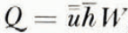
where Q (x, t) is the discharge in m.³ (ice)/yr. at time t through a fixed cross-section at x, and W is the glacier width.

It seems proper to use the density of ice in the net budget term

for time intervals of one year or more for the following reason: in general, the distribution of density with depth below the surface at any fixed point will be approximately constant in time if the density profile is always measured at the end of a budget year. This is an hypothesis similar to Sorge’s law for polar glaciers. In a steady-state condition an increment of snow of low density is added to the surface each year. This mass is compensated by an equal mass-increment of ice which flows out through the fixed cross-section (the mean density of the glacier is close to that of ice). Even though South Cascade Glacier is not currently in a steady-state condition, these relations must be approximately true because the process of compaction should proceed at about the same rate regardless of whether the glacier is in a steady or non-steady condition.

Values of Q calculated using equation (7) are presented in Figure 10; Q = 0 at the head of the glacier and reaches a peak of 8.8 × 10⁵ m.³/yr. at x = 2,320 m. The discharge then decreases almost to zero at the terminus. A slightly positive Q at the terminus is due to the discharge of ice into the lake by calving and melting. The discharge per meter of width, Q/W, is also shown in Figure 10. There is an apparent consistent relation between Q/W, and u (surface velocity averaged over the width). It should he noted that the Q/W and u results are entirely independent.

Fig. 10.

Longitudinal variations of discharge and velocity. Q is the actual discharge, Q/W is the discharge per unit width, Q₀/Q is the ratio of steady-state discharge to actual discharge, and u is the surface velocity averaged over the width. The values of Q and Q₀. were calculated using data averaged over the period 21 August 1958 to 12 September 1961

Glacier thickness

The mean thickness, h , of the glacier at each cross-section can be calculated from the relation

, where u is the velocity averaged over both width and depth. However, determining u exactly is difficult. The known surface velocity is made up of two components: one is due to the shear deformation within the ice and the other is the sliding velocity of the glacier on its bed. A minimum value for the mean depth can be computed by assuming that

. This assumption would be realistic if almost all of the velocity were due to sliding on the bed. The velocity distribution for ice obeying the Glen flow law, flowing in a channel of parabolic cross-section with the bed slip equal to zero is also such that

, according to a recent calculation by Nye (personal communication).

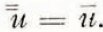
Slightly more precise thickness values might be computed by allowing for the decrease of velocity with depth. This can be done along the center line if the channel cross-section is known to approximate certain analytical shapes. However, the channel shape of South Cascade Glacier is not known, nor is there any obvious way to determine the decrease of velocity with depth away from the center line. Therefore, this calculation is not attempted here. It can be shown that the magnitude of the correction is small; nowhere can it exceed about 28 per cent.

A bedrock profile based on the assumption that

is shown in Figure 9. Qualitatively, the profile appears to be reasonable: flat uncrevassed areas occur where the bed profile is concave upwards; steep crevassed areas overlie convex parts of the bedrock profile. The maximum thickness (averaged over the width) is about 152 m.; the mean thickness for the whole glacier is about 83 m.

Relation to a steady-state condition

It is instructive to calculate how far the present condition of South Cascade Glacier differs from a steady state. One way to do this is to compute discharge which would result from a steady-state condition with the present glacier area and a steady-state net budget. First, a distribution of steady-state net budget values, b ₀, must be computed. Actual net budget values can he expressed as functions of elevation b(z). The net budget total, B, is obtained by multiplying the net budget values, b(z), by the corresponding distribution of area with altitude, S(z), and summing over the vertical extent of the glacier

By definition, a steady-state net budget is one in which

(Reference MeierMeier, 1962, p. 258). Therefore, a distribution of b ₀(z) can be obtained from any distribution of b(z) by subtracting B/S from each value of b(z), where S is the total area of the glacier, because

In Figure 5b, b ₀(z) and S(z) are graphed as functions of altitude. Curve 1 shows a b ₀(z) calculated from b(z) averaged over the whole period of record (budget years 1957–58 to 1963–64); curve 2 was computed using b(z) averaged for the period 21 August 1958 to 12 September 1961. Equation (3) was used in the averaging. The two curves are quite similar, even though the aberrant 1960–61 curve received much greater weight in curve 2.

A similar distribution of steady ,state net budget values can be obtained by summing over horizontal distance down-glacier, x, knowing the distribution of net budget, b(x), and area, S(x), with distance. A curve of b ₀(x) for the period 21 August 1958 to 12 September 1961 was used in equation (7) to calculate a steady-state unit discharge Q ₀(x)/W. This curve was calculated with an assumed discharge at the terminus equal to the present discharge. The resulting curve has a shape similar to the shape of the present unit discharge curve but the discharge at any given point is about twice as great. The ratio of Q ₀/Q is plotted as a function of x in Figure 10. This curve is dashed at the upper end (x < 400 m.), because here the computation of Q ₀ is sensitive to slight variations in the assumed b ₀. It is also dashed within 150 m. of the terminus, because the ratio has been arbitrarily forced to equal one at the terminus. This forcing has no appreciable effect more than 150 m. from the terminus. The mean ratio of Q ₀/Q is about 2.2. Reference NyeNye (1963[b]) also calculated values of Q ₀. His results differ from these by less than 6 per cent, although he used preliminary data and a different method of computation.

Although the calculated steady-state discharge of South Cascade Glacier is about twice the actual discharge, the calculated steady-state thickness is not twice as great, because

and the steady-state values

,

, and W ₀ would all be greater than under present conditions. From Nye’s analysis (Reference NyeNye, 1963[b], p. 112)

; so

, assuming W ₀ = W. This would suggest that the glacier would have to be about 16 per cent thicker than the present in order to have a steady-state discharge. However, the analysis is not as simple as this because, if the glacier is made thicker, the surface slope must change, decreasing the velocity in the upper part of the glacier and increasing it at the terminus, necessitating increased thickness above and decreased thickness below. The width of the glacier will be slightly increased and the changed elevation of the glacier surface will cause the distribution of net budget values to change. Calculation of an internally consistent steady-state profile of the glacier is laborious, requires many simplifying assumptions and is not attempted here. However, it appears that the glacier would have to he somewhat less than 16 per cent thicker in order to handle a steady-state distribution of net budget with the present-day length and area.

Acknowledgements

We wish to thank Dr. J. F. Nye and E. R. LaChapelle for helpful discussion and critical reading of the manuscript.