



1 Introduction & preliminaries
1.1 Introduction
While many of the properties of types have generalizations to the context of measures (e.g., invariance, definability, and finite satisfiability), the machine that is model theory interacts with these objects differently. The central difference is that you can’t realize a measure, in a strong sense. Measures are not realized in some elementary extension the way types can be realized. Granted, a lot can be accomplished in this setting, but some powerful classical tools are missing. One striking difference is the lack of arguments using indiscernible sequences. This is because, in a strict sense, indiscernible sequences do not exist for measures.
The power of the randomization [Reference Ben Yaacov and Keisler6, Reference Keisler22] is that it provides a framework in which one can realize a measure, if you are willing to change your underlying structure to a closely related one, and also learn a smidgen of continuous logic. Instead of working with measures directly, one now works with random variables (or random elements) taking values in our original structure. In an important (yet unpublished) research note, Ben Yaacov describes how to turn global Keisler measures into types over a monster model of the randomization. These transfer methods allow one to turn questions involving measures into those involving types (in continuous logic). This perspective restores access to a lot of model-theoretic machinery, including important portions of neostability [Reference Andrews, Goldbring and Keisler2, Reference Ben Yaacov3, Reference Ben Yaacov and Keisler6, Reference Ben Yaacov and Usvyatsov7, Reference Conant, Gannon and Hanson18, Reference Khanaki23]. More importantly, this perspective is practical and we can prove new results about measures (this is often the case with particular kinds of convergence problems—see [Reference Hrushovski, Pillay and Simon21, Lemma 2.10] via [Reference Ben Yaacov3], or [Reference Chernikov, Gannon and Krupiński12, Proposition 3.23]).
The Morley product is a fundamental construction in model theory, for both types and measures [Reference Hrushovski, Pillay and Simon21]. When it exists, this product glues measures together in a generic/non-forking way. This product plays an important role in combinatorial results [Reference Chernikov and Starchenko14, Reference Simon25], convolution algebras and dynamical systems [Reference Chernikov and Gannon10–Reference Chernikov, Gannon and Krupiński12], as well as certain kinds of probability spaces [Reference Gannon and Hanson19]. Understanding precisely how the Morley product interacts with the transfer maps gives us access to more tools to better analyze these constructions and contexts.
The results here are primarily about the connections between measures and random types over NIP structures. We will assume that our underlying theory T is both countable and NIP throughout. For some technical reasons, we focus here on the case of finitely satisfiable measures instead of the more general setting of invariant measures. Even though we make this general assumption, we try our best to specify precisely where we use the NIP and finite satisfiability assumptions. We do the following:
-
(1) Basic observations: We verify some of the claims in Ben Yaacov’s note [Reference Ben Yaacov4]. We also make some basic observations.
-
(2) Going up: Assuming NIP, we prove that the Morley product commutes with transfer map.
-
(3) Going down: We observe that the restriction map does not commute with the Morley product. We provide a condition on pairs of finitely satisfiable types which ensures commutativity.
-
(4) Over a group: The transfer map is an injective embedding of topological semigroups from the convolution algebra of Keisler measures to types over the randomization (under the Newelski product). If our group is definably amenable, then the minimal left ideal in the space of finitely satisfiable types over the randomization is a single point. We had hoped that the transfer map would provide an isomorphism on the level of minimal left ideals in the general NIP setting. However, we show that if our underlying group is not definably amenable, then the minimal left ideal in the Ellis semigroup of random finitely satisfiable types is somehow always more complicated than the minimal left ideal in the convolution algebra.
1.2 Preliminaries
We assume some familiarity with Keisler measures, randomizations, basic continuous logic, etc. Fix a first-order theory T in a countable language
 $\mathcal {L}$
. We briefly recall the construction of easy models of the randomization. Let
 $(\Omega _0, \mathcal {B}_0,\mathbb {P}_0)$
denote an atomless probability algebra with event space
 $\Omega _0$
,
 $\sigma $
-algebra
 $\mathcal {B}_0$
, and probability measure
 $\mathbb {P}_0$
. Then any model
 $M\models T$
gives rise to a model
 $M^{(\Omega _0,\mathcal {B}_0,\mathbb {P}_0)}$
of the randomization of T, denoted
 $T^{R}$
. We will write
 $M^{(\Omega _0,\mathcal {B}_0,\mathbb {P}_0)}$
simply as
 $M^{\Omega }$
. We recall its construction. First define
 $$\begin{align*}M_0^\Omega := \{f\colon \Omega_0 \to M: f \text{ is } \mathcal{B}_0\text{-measurable and has finite image}\}. \end{align*}$$
Notice that
 $M^{\Omega }_0$
has a natural pseudo-metric given by
 $d(f,g) = \mathbb {P}_0(\{ t \in \Omega _0 : f(t) \neq g(t)\})$
. Then
 $M^{\Omega }$
is constructed by quotienting by distance
 $0$
and taking the metric completion on the quotient. Likewise,
 $\mathcal {B}_0$
is a pseudo-metric space, with distance given by
 $d(A,B) = \mathbb {P}_0(A \triangle B)$
. Again, we identify measurable sets up to measure
 $0$
and take the metric completion. Then the randomization
 $(M^\Omega ,\mathcal {B})$
is the two sorted structure in the language
 $\mathcal {L}^{R}$
which is the disjoint union of the language of probability algebras on the second sort and a collection of functions,
 $\{[\varphi (\bar {x})]: \varphi (\bar {x})$
is an
 $\mathcal {L}$
-formula
 $\}$
, from the random element sort to the probability algebra sort. More explicitly,
-
(1)
 $\mathcal {B}$
retains the structure of a probability algebra in the language
$\{\mathbb {P}, \cap , \cup , ^{c}, \perp , \top \}$
. In particular, formulas are extended from
$\mathcal {B}_0$
to
$\mathcal {B}$
via continuity.
-
(2) For every
$\mathcal {L}$
-formula
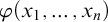
$\varphi (x_1,\ldots ,x_n)$
, we have a function
$[\varphi (x_1,\ldots ,x_n)]:(M_0^{\Omega })^{n} \to \mathcal {B}_0$
via This is extended by continuity to
$$ \begin{align*} [\varphi(h_1,\ldots,h_n)] = \{t \in \Omega_0 : M \models \varphi(h_1(t),\ldots,h_n(t))\}. \end{align*} $$
$(M^{\Omega },\mathcal {B})$
.
-
(3) Putting
$(1)$
and
$(2)$
together; for any
$\mathcal {L}$
-formula
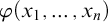
$\varphi (x_1,\ldots ,x_n)$
we have a function
$\mathbb {E}[\varphi (x_1,\ldots ,x_n)]:(M_0^{\Omega })^{n} \to [0,1]$
via Again, this is extended by continuity to
$$ \begin{align*} \mathbb{E}[\varphi(h_1,\ldots,h_n)] = \mathbb{P}_0(\{t \in \Omega_0: M \models \varphi(h_1(t),\ldots,h_n(t))\}). \end{align*} $$
$(M^{\Omega },\mathcal {B})$
. We often only need to work with
$\mathcal {L}^{R}$
-formulas of the form
$\mathbb {E}[\varphi (x_1,\ldots ,x_n)]$
.











Formally, one can define the theory of the randomization of T,
 $T^{R}$
, as the theory of
 $(M^{\Omega },\mathcal {B})$
in the language
 $\mathcal {L}^{R}$
for any choice of model of T and any atomless probability algebra
 $(\Omega _0,\mathcal {B}_0,\mathbb {P}_0)$
[Reference Ben Yaacov and Keisler6]. By construction, the structure
 $(M_0^\Omega ,\mathcal {B}_0)$
is a metrically dense (pre-)substructure of
 $(M^{\Omega },\mathcal {B})$
. Throughout this article, we will usually refer to an easy model by its random element sort, e.g.,
 , and leave the probability algebra sort implicit.
We remark that if
 $\mathcal {U}$
is a monster model of T, then the model
 is usually not saturated and so we will always think of
 as elementarily embedded in a monster model of
 $T^{R}$
, i.e.,
 . As convention, we write
 to mean
 $b \in \hat {\mathcal {K}}_{C}$
as well as
 to mean that p is a global type in the random element sort, i.e.,
 .
If
 $h \in \mathcal {U}^{\Omega }_0$
, then a partition for h is a finite
 $\mathcal {B}_0$
-measurable partition of
 $\Omega _0$
, say
 $\mathcal {A}$
, such that for any
 $A \in \mathcal {A}$
,
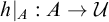 $h|_{A}: A \to \mathcal {U}$
is a constant function. We let
 $h|_{A}$
denote the unique element in
 $\mathcal {U}$
such that for any
 $t \in A$
,
 $h(t) = h|_{A}$
. By elementarity, one can interpret the set
 $\mathcal {A}$
as also a partition of the probability algebra associated with
 , i.e.,
 $\mathcal {B}_{C}$
. If
 $b \in \mathcal {U}$
, we let
 $f_{b}: \Omega _0 \to \mathcal {U}$
define the random variable which takes constant value b, i.e., for any
 $t \in \Omega _0$
,
 $f_b(t) = b$
.
Our set up is as follows: Let M be a model of T, and let
 $\mathcal {U}$
be a monster model of T such that
 $M \prec \mathcal {U}$
. Then we have that
 (by quantifier elimination, see Remark 1.5). We now consider a monster model
 of
 $T^{R}$
such that
 . We are interested in the connection between global types in the random element sort which are finitely satisfiable over the structure
 , denoted
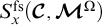 and global Keisler measures which are finitely satisfiable over M, denoted
 $\mathfrak {M}_{x}^{\mathrm {fs}}(\mathcal {U},M)$
. We let
 $\mathfrak {M}_{x}(\mathcal {U})$
be the collection of all Keisler measures over
 $\mathcal {U}$
. As stated previously, we assume that the reader has some knowledge of Keisler measures, however, we take a moment to recall some basic definitions and conventions.
Definition 1.1. Let M be a small elementary submodel of
 $\mathcal {U}$
and
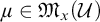 $\mu \in \mathfrak {M}_{x}(\mathcal {U})$
.
-
(1) The measure
$\mu $
is M-invariant if for any
$a, b \in \mathcal {U}^{ y }$
such that
$ a \equiv _{M} b$
and for any
$\mathcal {L}$
-formula
$\varphi (x, y)$
, we have that
$\mu (\varphi ( x, a)) = \mu (\varphi ( x, b))$
. We let
$\mathfrak {M}_{ x}^{\mathrm {inv}}(\mathcal {U},M)$
be the collection of measures in
$\mathfrak {M}_{ x}(\mathcal {U})$
which are M-invariant. -
(2) Let
$\mu \in \mathfrak {M}^{\mathrm {inv}}_{x}(\mathcal {U},M)$
. Then for any
$\mathcal {L}_{x}(M)$
-formula
$\varphi (x, y)$
, we can define the map
$F_{\mu ,M}^{\varphi }\colon S_{y}(M) \to [0,1]$
via
$F_{\mu ,M}^{\varphi }(q) = \mu (\varphi ( x, b))$
where
$ b \in \mathcal {U}^{{y}}$
such that
$b \models q$
. We remark that this map is well-defined since
$\mu $
is M-invariant. -
(3) The measure
$\mu $
is finitely satisfiable in M if for any
$\mathcal {L}_{x}(\mathcal {U})$
-formula
$\varphi (x)$
, if
$\mu (\varphi (x))> 0$
then there exists some
$a \in M$
such that
$\mathcal {U} \models \varphi (a)$
. As mentioned above, we let
$\mathfrak {M}_{x}^{\mathrm {fs}}(\mathcal {U},M)$
be the collection of measures in
$\mathfrak {M}_{x}(\mathcal {U})$
which are finitely satisfiable in M. It is straightforward to check that
$\mathfrak {M}_{x}^{\mathrm {fs}}(\mathcal {U},M) \subseteq \mathfrak {M}_{x}^{\mathrm {inv}}(\mathcal {U},M)$
. -
(4) Let
$\mu \in \mathfrak {M}^{\mathrm {inv}}_{ x}(\mathcal {U},M)$
. We say that
$\mu $
is Borel-definable (over M) if for every
$\mathcal {L}$
-formula
$\varphi ( x, y)$
, the map
$F_{\mu ,M}^{\varphi }$
is a Borel function. -
(5) Let
$\mu \in \mathfrak {M}^{\mathrm {inv}}_{ x}(\mathcal {U},M)$
. We say that
$\mu $
is definable (over M) if for every
$\mathcal {L}$
-formula
$\varphi ( x, y)$
, the map
$F_{\mu ,M}^{\varphi }$
is a continuous function. -
(6) Let
$\mu \in \mathfrak {M}^{\mathrm {inv}}_{ x}(\mathcal {U},M)$
and
$\nu \in \mathfrak {M}_{ y}(\mathcal {U})$
. Suppose that
$\mu $
is Borel-definable over M. We define the Morley product
$\mu \otimes \nu $
on
$\mathcal {L}_{x y}(\mathcal {U})$
as follows: For any formula
$\varphi ( x, y) \in \mathcal {L}_{ x y}(\mathcal {U})$
, we have that where N is any small elementary submodel containing M and all the parameters from
$$ \begin{align*} (\mu \otimes \nu)(\varphi( x, y)) = \int_{S_{ y}(N)} F_{\mu,N}^{\varphi}\, d\nu|_{N}, \end{align*} $$
$\varphi $
and
$\nu |_{N}$
is the unique regular Borel probability measure on
$S_{y}(N)$
corresponding to the restriction of
$\nu $
to
$\mathcal {L}_{y}(N)$
. We remark that this product is well-defined and
$\mu \otimes \nu \in \mathfrak {M}_{{x}{y}}(\mathcal {U})$
(see [Reference Simon24, p. 106]). In practice, we always drop the N from the notation, e.g., we write
$F_{\mu }^{\varphi }$
instead of
$F_{\mu ,N}^{\varphi }$
and
$\nu $
instead of
$\nu |_{N}$
.



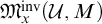



























We recall the maps between Keisler measures and types over the randomization. Our first map is the restriction map from  to
 $\mathfrak {M}_{x}(\mathcal {U})$
.
Definition 1.2. We define the map  where for any
 ,
 $$ \begin{align*} \nu_{q}(\varphi(x,b_1,\ldots,b_n)) = (\mathbb{E}[\varphi(x,f_{b_1},\ldots,f_{b_n})])^{q}. \end{align*} $$
Proposition 1.3. The map  is continuous.
Proof. Notice that if O is a basic open set in
 $\mathfrak {M}_{x}(\mathcal {U})$
, then
 $$ \begin{align*} O=\bigcap_{i=1}^{n} \{\mu \in \mathfrak{M}_{x}(\mathcal{U}):r_{i}<\mu(\varphi_{i}(x,b_{i}))<s_{i}\}, \end{align*} $$
where
 $r_1,\ldots ,r_n,s_1,\ldots ,s_n$
are real numbers,
 $b_1,\ldots ,b_n$
are parameters from
 $\mathcal {U}$
, and
 $\varphi _1(x,y),\ldots ,\varphi _n(x,y)$
are
 $\mathcal {L}$
-formulas. Then

which is clearly open.
The following two constructions are essentially from [Reference Ben Yaacov4], the only caveat being that the map
 $r_{-}$
(Definition 1.4) has codomain over the monster model. We also mention that the map
 $r_{-}$
was explicitly studied in [Reference Conant, Gannon and Hanson18]. Ben Yaacov calls the following map the natural extension.
Definition 1.4. Let
 $\mu \in \mathfrak {M}_{x}(\mathcal {U})$
and suppose that
 $\mu $
is definable over M. Then there exists a unique type
 such that for every
 and
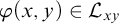 $\varphi (x,y) \in \mathcal {L}_{xy}$
,
 $$ \begin{align*} (\mathbb{E}[\varphi(x,b)])^{r_{\mu}} = \lim_{i \in I} \sum_{A \in \mathcal{A}_i} \mathbb{P}_0(A) \mu(\varphi(x,h_i|_{A})). \end{align*} $$
where
 $(h_i,\mathcal {A})_{i \in I}$
is any indexed family such that:
-
(1) For each
$i \in I$
,
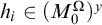
$h_i \in (M_{0}^{\Omega })^{y}$
. -
(2) For each
$i \in I$
,
$\mathcal {A}_i$
is a partition for
$h_i$
. -
(3)
.



 .
The following tools will aid us in our computations.
Remark 1.5.
-
(1) Equivalence of invariance and Borel-definability in NIP theories [Reference Hrushovski and Pillay20, Corollary 4.9]. Suppose that T is NIP and
$\mu \in \mathfrak {M}_{x}(\mathcal {U})$
. Then
$\mu $
is M-invariant if and only if
$\mu $
is Borel-definable over M. -
(2) Associativity of the Morley product of definable measures in arbitrary theories [Reference Conant and Gannon15, Proposition 2.6]. Suppose that T is arbitrary and
$\mu \in \mathfrak {M}_{x}(\mathcal {U})$
,
$\nu \in \mathfrak {M}_{y}(\mathcal {U})$
, and
$\lambda \in \mathfrak {M}_{x}(\mathcal {U})$
. If
$\mu $
and
$\nu $
are definable over a small model then
$(\mu \otimes (\nu \otimes \lambda )) = ((\mu \otimes \nu ) \otimes \lambda )$
. -
(3) Associativity of invariant measures in NIP theories [Reference Conant and Gannon16, Theorem 2.2]. Suppose that T is NIP and
$\mu \in \mathfrak {M}_{x}(\mathcal {U})$
,
$\nu \in \mathfrak {M}_{y}(\mathcal {U})$
, and
$\lambda \in \mathfrak {M}_{x}(\mathcal {U})$
. If
$\mu $
and
$\nu $
are invariant over a small model then
$(\mu \otimes (\nu \otimes \lambda )) = ((\mu \otimes \nu ) \otimes \lambda )$
. -
(4) Left-continuity of the Morley product for invariant measures in NIP theories [Reference Chernikov and Gannon10, Theorem 6.3]. Suppose that T is NIP,
$\nu \in \mathfrak {M}_{x}(\mathcal {U})$
, and
$\varphi (x,y) \in \mathcal {L}_{xy}(\mathcal {U})$
. Then
$- \otimes \nu (\varphi (x,y)) : \mathfrak {M}_{x}^{\mathrm {fs}}(\mathcal {U},M) \to [0,1]$
is continuous. As a consequence, the map
$-\otimes \nu : \mathfrak {M}_{x}^{\mathrm {fs}}(\mathcal {U},M) \to \mathfrak {M}_{xy}(\mathcal {U})$
is continuous. -
(5) Right-continuity of the Morley product for definable measures in arbitrary theories (see, e.g., [Reference Conant, Gannon and Hanson17, Lemma 5.4]). Suppose that T is arbitrary,
$\mu \in \mathfrak {M}_{x}(\mathcal {U})$
is definable, and
$\varphi (x,y) \in \mathcal {L}_{xy}(\mathcal {U})$
. Then
$\mu \otimes - (\varphi (x,y)) : \mathfrak {M}_{y}(\mathcal {U}) \to [0,1]$
is continuous. -
(6) Quantifier elimination in the randomization (i.e., [Reference Ben Yaacov and Keisler6]).
$T^{R}$
has quantifier elimination. In particular, any type is completely determined by the values of
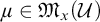














 is completely determined by the values of

The following map was also defined in [Reference Ben Yaacov4]. Ben Yaacov refers to it as extension-by-definition. This article will primarily focus on this map. We remark that [Reference Ben Yaacov4] defines the map for all Borel-definable measures. However, we only claim to verify that the types defined below are consistent under the additional hypothesis that our measures are in the NIP + finitely satisfiable context. Thus, we have changed the definition to fit our context.
Definition 1.6 (T NIP).
Let
 $\mu \in \mathfrak {M}_{x}^{\mathrm {fs}}(\mathcal {U},M)$
. Then there exists a unique type
 such that for every
 , and
 $\varphi (x,z) \in \mathcal {L}_{xz}$
,

2 Basic observations
For the rest of the article, we fix M,
 $\mathcal {U}$
models of T such that
 $M \prec \mathcal {U}$
and
 $\mathcal {U}$
is a monster model of T. We let
 $(\Omega _0,\mathcal {B}_0,\mathbb {P}_0)$
be a fixed atomless probability space and so
 is fixed. Finally, we fix a monster model
 of the randomization
 . We list the known results connected to transfer properties. The following statements are true. Many appear in either [Reference Ben Yaacov4] or [Reference Conant, Gannon and Hanson18].
-
(a) Suppose that
$\mu \in \mathfrak {M}_{x}(\mathcal {U})$
and
$\mu $
is definable over M. Then
$r_{\mu } = s_{\mu }$
(observed in [Reference Ben Yaacov4], without proof). We take the opportunity to provide one. This is true when both
$r_{\mu }$
and
$s_{\mu }$
are well-defined and does not require NIP. -
(b) The map
$\nu _{-}$
preserves invariance, definability, finite satisfiability, and fam. These are quite straightforward and we write them down here. -
(c) The map
$r_{-}$
preserves definability, fam, and fim. Definability was proved in [Reference Ben Yaacov4] while fim and fam were proved in [Reference Conant, Gannon and Hanson18]. -
(d) (T NIP) The map
$s_{-}$
preserves finite satisfiability. This was proved in [Reference Ben Yaacov4] and we give another proof here. By Statements
$(a)$
and
$(c)$
,
$s_{-}$
preserves definability and generic stability as well.


In this section, we give proofs of the following, in the order listed:
-
(1) A proof of Statement (a).
-
(2) Under NIP, if
$\mu \in \mathfrak {M}_{x}^{\mathrm {fs}}(\mathcal {U},M)$
, then
$s_{\mu }$
is consistent and finitely satisfiable in . The latter is done in [Reference Ben Yaacov4] and our proof is a different style. -
(3) We provide a proof of Statement (b).


 . The latter is done in [
We first prove that the maps
 $r_{-}$
and
 $s_{-}$
agree on definable measures. We recall a basic fact.
Fact 2.1. If
 $h \in \mathcal {U}^{\Omega }_0$
and
 $\mathcal {A}$
is a partition for h, then
 .
Proof. Fix
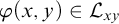 $\varphi (x,y) \in \mathcal {L}_{xy}$
and
 $b \in \mathcal {U}^{y}$
. Notice,

Proposition 2.2. Suppose
 $\mu \in \mathfrak {M}_{x}(\mathcal {U})$
and
 $\mu $
is definable over M. Then
 $r_{\mu } = s_{\mu }$
.
Proof. Fix
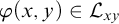 $\varphi (x,y) \in \mathcal {L}_{xy}$
and
 . Fix
 $(h_i, \mathcal {A}_{i})_{i \in I}$
such that for each
 $i \in I$
we have
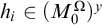 $h_i \in (M^{\Omega }_0)^{y}$
,
 $\mathcal {A}_{i}$
is partition for
 $h_i$
, and
 . Consider the following computation:

By quantifier elimination,
 $r_{\mu } = s_{\mu }$
. We provide the following justifications:
-
(a) Since
$r_{\mu }$
is definable, the map is continuous and so commutes with nets. -
(b) For fixed i, the value of the left-hand side of the equality is precisely the value of the right-hand side of the equality.
-
(c) Follows directly from Fact 2.1.
-
(d) Application of Remark 1.5(5). More explicitly, note that
-
(e) The map
is continuous and so commutes with nets. -
(f) Recall that the integral is respect to the restriction of the measure to the space in the integrand. Thus it suffices to show that for any
$\theta (x,m) \in \mathcal {L}_{y}(M)$
, we have that . This follows directly by our hypothesis for choice of
$h_i$
’s.

 is continuous and so commutes with nets.

 is continuous and so commutes with nets.

 . This follows directly by our hypothesis for choice of

In [Reference Conant, Gannon and Hanson18], we (along with Conant and Hanson) verified that if
 $\mu $
is definable, then the type
 $r_{\mu }$
is consistent [Reference Conant, Gannon and Hanson18, Fact 3.10]. In the following, we use a simpler version of this statement, i.e., that if
 $a_1,...,a_n$
is a sequence of elements in M, then the type
 $r_{\mathrm {Av}(\bar {a})}$
is consistent. We provide a quick proof.
Fact 2.3. Suppose that
 $a_1,\ldots ,a_n$
is a sequence of elements in M. Then the type
 $r_{\mathrm {Av}(\bar {a})}$
is consistent.
Proof. We give a sketch. By quantifier elimination, we have  (see [Reference Berenstein and Muñoz8, Proposition 3.11] for direct proof). More explicitly, our probability space is
 $(\Omega _0 \times [0,1), \mathcal {B}_0 \times \mathcal {B}_{[0,1)},\mathbb {P}_{0} \times L)$
where L is the Lebesgue measure and
 $\mathcal {B}_{[0,1)}$
is the collection of Borel subsets of
 $[0,1)$
. Consider the element
 $h_{\bar {a}} \in \mathcal {U}^{\mathcal {B} \times [0,1]}$
where
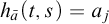 $h_{\bar {a}}(t,s) = a_j$
whenever
 $s \in [\frac {j-1}{n},\frac {j}{n})$
. Let
 $q = \operatorname {tp}(h_{\bar {a}}/\mathcal {U}^{\Omega })$
. We claim that q is definable over
 $\mathcal {U}^{\Omega }$
. Indeed, for any
 $\mathcal {L}$
-formula
 $\varphi (x,y)$
and any
 $b \in \mathcal {U}_0^{\Omega }$
, we have the following computation:
 $$ \begin{align*} (\mathbb{E}[\varphi(x,b)])^{q} &= \mathbb{E}[\varphi(h_{\bar{a}},b)] \\ &= \mathbb{P}_0 \times L \left(\left\{ (t,s) \in \Omega_0 \times [0,1) : \mathcal{U} \models \varphi(h_{\bar{a}}(t,s), b(t,s)) \right\} \right) \\ &=\sum_{i=1}^{n} \mathbb{P}_0 \times L \left(\left\{ (t,s) \in \Omega_0 \times \left[\frac{i-1}{n},\frac{i}{n} \right) : \mathcal{U} \models \varphi(h_{\bar{a}}(t,s), b(t,s)) \right\} \right) \\ &=\sum_{i=1}^{n} \mathbb{P}_0 \times L \left(\left\{ (t,s) \in \Omega_0 \times \left[\frac{i-1}{n},\frac{i}{n} \right) : \mathcal{U} \models \varphi(a_i, b(t)) \right\} \right) \\ &=\sum_{i=1}^{n} \frac{1}{n} \mathbb{P}_0 \left(\left\{ t \in \Omega_0 : \mathcal{U} \models \varphi(a_i, b(t) \right\} \right) \\ &=\sum_{i=1}^{n} \frac{1}{n} \mathbb{E}[\varphi(f_a,b)]. \end{align*} $$
Using a moduli of continuity argument, one can show that for every
 $b \in \mathcal {U}^{\Omega }$
,
 $(\mathbb {E}[\varphi (x,b)])^{q} = \sum _{i=1}^{n} \frac {1}{n} \mathbb {E}[\varphi (f_a,b)]$
. Thus q is definable and we let
 $\hat {q}$
be the unique definable extension of q to
 . We leave it to the reader to verify that
 $\hat {q} = r_{\mathrm {Av}(\bar {a})}$
.
Proposition 2.4 (T NIP).
For any
 $\mu \in \mathfrak {M}_{x}^{\mathrm {fs}}(\mathcal {U},M)$
, the type
 $s_{\mu }$
is consistent and finitely satisfiable in
 .
Proof. We first show that the type
 $s_{\mu }$
is consistent. Fix
 $\mathcal {L}$
-formulas
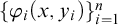 $\{\varphi _{i}(x,y_i)\}_{i=1}^{n}$
and
 $b_1,\ldots ,b_n$
from
 , and
 $\epsilon> 0$
. By quantifier elimination, it suffices to show that there exists a type
 such that
 $$ \begin{align*} |(\mathbb{E}[\varphi_i(x,b_i)])^{q} - (\mathbb{E}[\varphi_i(x,b_i)])^{s_{\mu}}| < \epsilon. \end{align*} $$
Since
 $\mu $
is finitely satisfiable in M, there exists a net of measures
 $(\mu _j)_{j \in J}$
such that
 $\mu _j = \mathrm {Av}(\bar {a}_{j}) \in \operatorname {conv}(M)$
and
 $\lim _{j \in J} \mu _{j} = \mu $
. Notice that for each
 $i \leq n$
,

Equation
 $(*)$
holds by Remark 1.5(4). Since for each
 $i \leq n$
, the map
 via
 $p \to (\mathbb {E}[\varphi _i(x,b_i)])^{p}$
is continuous, we can find some
 $j \in J$
such that for each
 $i \leq n$
,
 $$ \begin{align*} |\mathbb{E}[\varphi_i(x,b_i)]^{s_{\mathrm{Av}(\bar{a}_j)}} - \mathbb{E}[\varphi_i(x,b_i)]^{s_{\mu}}| < \epsilon. \end{align*} $$
Since
 $s_{\mathrm {Av}(\bar {a}_j)} = r_{\mathrm {Av}(\bar {a}_j)}$
(by Proposition 2.2) and
 $r_{\mathrm {Av}(\bar {a}_j)}$
is a consistent type (by Fact 2.3), the type
 $s_{\mu }$
is consistent.
We now argue that
 $s_{\mu }$
is finitely satisfiable in
 . For each
 $j \in J$
, the type
 $r_{\mathrm {Av}(\overline {a}_j)}$
is generically stable over
 (see [Reference Conant, Gannon and Hanson18, Corollary 3.19]) and this implies that
 $r_{\mathrm {Av}(\overline {a}_j)}$
is finitely satisfiable in
 . Since the collection of types which are finitely satisfiable in
 is a closed set and
 $\lim _{j \in J} s_{\mathrm {Av}(\bar {a}_j)} = s_{\mu }$
, we conclude that
 $s_{\mu }$
is also finitely satisfiable in
 .
Proposition 2.5. If T is NIP, then the map  is continuous.
Proof. Similar to the proof above. Let
 $(\mu _i)_{i \in I}$
be a net of elements in
 $\mathfrak {M}_{x}^{\mathrm {fs}}(\mathcal {U},M)$
such that
 $\lim _{i \in I} \mu _i = \mu $
. It suffices to prove that
 $\lim _{i \in I} s_{\mu _i} = s_{\mu }$
. By quantifier elimination, it suffices to show that these terms agree on all atomic formulas. Let
 $\varphi (x,y)$
be an
 $\mathcal {L}$
-formula and
 . Then

We remark that Equation
 $(*)$
follows from Remark 1.5(4).
The next proposition is useful in proving that the restriction of a definable type in the randomization yields a definable measure, but seems slightly important in its own right.
Proposition 2.6. Consider the map  where if
 $a \models q$
, then
 . This map is well-defined and continuous.
Proof. Well-definedness follows quickly from an automorphism argument. Let
 $a,b \models p$
and
 $\sigma \in \operatorname {Aut}( \mathcal {U}/M)$
map
 $a \to b$
. Then
 $\sigma $
extends to an automorphism
 which maps
 $f_{a}$
to
 $f_{b}$
. More explicitly,
 $\sigma '$
is the identity on the probability algebra sort and for any
 $h \in \mathcal {U}^{\Omega }_0$
, we have that
 $\sigma '(h) = \sigma \circ h$
.
 $\sigma '$
is extended to
 $\mathcal {U}^{\Omega }$
via continuity.
We now argue that f is continuous. Suppose that
 $\lim _{i \in I} p_i = p$
. Let
 $a_i \models p_i$
and
 $a \models p$
. It suffices to prove that for each formula
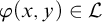 $\varphi (x,y) \in \mathcal {L}$
and
 $h \in M^{\Omega }_0$
that
 $\lim _{i \in I} \mathbb {E}[\varphi (x,h)]^{\operatorname {tp}(f_{a_i}/M)} = \mathbb {E}[\varphi (x,h)]^{\operatorname {tp}(f_{a}/M)}$
. Fix a partition
 $\mathcal {A}$
for h. Now notice that

Proposition 2.7. Suppose  .
-
(1) If q is
-invariant, then
$\nu _{q}$
is M-invariant. -
(2) If q is finitely satisfiable in
, then
$\nu _{q}$
is finitely satisfiable in M. -
(3) If q is
-definable, then
$\nu _{q}$
is M-definable. -
(4) If q is fam over
, then
$\nu _{q}$
is fam over M.
 -invariant, then

 , then

 -definable, then

 , then

Proof. We prove the statements:
-
(1) Let
$a,b \in \mathcal {U}^{y}$
and suppose that
$\operatorname {tp}(a/M) = \operatorname {tp}(b/M)$
. Then there exists an automorphism
$\sigma : \mathcal {U} \to \mathcal {U}$
which fixes M and maps
$a \to b$
. Again, we claim that
$\sigma ':\mathcal {U}_0^{\Omega } \to \mathcal {U}_0^{\Omega }$
via
$\sigma '(h) = \sigma \circ h$
is an automorphism of fixing . Now,
$$ \begin{align*} \nu_{q}(\varphi(x,a)) = (\mathbb{E}[\varphi(x,f_{a})])^{q} &= (\mathbb{E}[\varphi(x,\sigma'(f_a))])^{q} \\ &= (\mathbb{E}[\varphi(x,f_{b})])^{q} = \nu_{q}(\varphi(x,b)). \end{align*} $$
-
(2) Suppose that
$\nu _{q}(\varphi (x,b))> 0$
. Then
$(\mathbb {E}[\varphi (x,f_{b})])^{q}> 0$
. So, there exists some
$h \in M_0^{\Omega }$
such that
$(\mathbb {E}[\varphi (h,f_{b})])> 0$
. If
$\mathcal {A}$
is a partition for h, then and so there is some
$$ \begin{align*} 0< (\mathbb{E}[\varphi(h,f_{b})]) &= \mathbb{P}_0 \Big( \Big\{ t \in \Omega_0: \mathcal{U} \models \varphi(h(t_*),b) \Big\} \Big). \\ &=\sum_{A \in \mathcal{A}}\mathbb{P}_0(A)\mathbf{1}_{\varphi(x,y)}(h|_{A},b), \end{align*} $$
$A_* \in \mathcal {A}$
such that
$\models \varphi (h|_{A*},b)$
.
-
(3) Fix an
$\mathcal {L}$
-formula
$\varphi (x,y)$
. Consider
$(p_i)_{i \in I}$
and p in
$S_{y}(M)$
such that
$\lim _{i \in I} p_i = p$
. It suffices to show that
$\lim _{i \in I} F_{\nu _{q}}^{\varphi }(p_i) = F_{\nu _{q}}^{\varphi }(p)$
. Fix
$(c_i)_{i \in I}$
and c in
$\mathcal {U}$
such that
$c_i \models p_i$
and
$c \models p$
. By Fact 2.6, . Now notice that where Equation
$(*)$
follows from definability of q.
-
(4) Fix an
$\mathcal {L}$
-formula
$\varphi (x,y)$
and
$\epsilon> 0$
. Since p is fam over , there exists
$h_1,\ldots ,h_n \in M^{\Omega }_0$
such that For each
$i \leq n$
, choose a partition
$\mathcal {A}_i$
for
$h_i$
. Now for any
$b \in \mathcal {U}$
, The final term can be approximated by a measure of the form
$$ \begin{align*} \nu_{p}(\varphi(x,b)) &= (\mathbb{E}[\varphi(x,f_b)])^{p}\\ &\approx_{\epsilon} \frac{1}{n}\sum_{i \leq n} \mathbb{E}[\varphi(h_i,f_{b})] \\ &= \frac{1}{n} \sum_{i \leq n} \mathbb{P}_0\left( \{t \in \Omega_0: \mathcal{U} \models \varphi(h_i(t),b) \} \right) \\ &= \frac{1}{n} \sum_{i \leq n} \sum_{A \in \mathcal{A}_i} \mathbb{P}_0(A) \mathbf{1}_{\varphi(x,y)}(h_i|_{A},b) \\ &= \left( \frac{1}{n}\sum_{i \leq n}\sum_{A \in \mathcal{A}_i} \mathbb{P}_0(A)\delta_{\operatorname{tp}(h_i|_{A}/\mathcal{U})} \right) (\varphi(x,b)). \end{align*} $$
$\mathrm {Av}(\overline {c})$
where each
$c_i$
appears in
$\bigcup _{i=1}^{n}\{h_i|_{A}: A \in \mathcal {A}_i\}$
. Indeed, the only issue is that
$\mathbb {P}(A)$
may be irrational and so choosing a small enough rational approximation completes the proof.




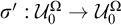

 fixing
 . Now,







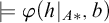






 . Now notice that


 , there exists





The following question remains open.
Question 2.8. Let  . Suppose that q is generically stable over
 . Does this imply that
 $\nu _{q}$
is fim? We remark that if the answer is ‘Yes’, this answers an open question from [Reference Conant, Gannon and Hanson18].
Proposition 2.9. Let
 $\mu \in \mathfrak {M}^{\mathrm {fs}}_{x}(\mathcal {U},M)$
. Then
 $\nu _{s_{\mu }} = \mu $
.
Proof. Fix
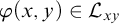 $\varphi (x,y) \in \mathcal {L}_{xy}$
and
 $b \in \mathcal {U}^{y}$
. Then

Warning. We remark that in general,
 $s_{\nu _{q}} \neq q$
. In particular, the map
 $\nu _{-}$
is far from being injective. Fix any
 $A \subseteq \Omega _0$
such that
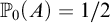 $\mathbb {P}_0(A) = 1/2$
and
 $b_1,b_2 \in M$
. Consider the random element
 $g:\Omega \to \mathcal {U}$
where
 $$ \begin{align*} g(t)=\begin{cases} \begin{array}{@{}cc} b_{1} & t\in A,\\ b_{2} & t\in A^{c}. \end{array}\end{cases} \end{align*} $$
Notice that 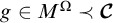 . For any choice of such A,
 .
3 Going up: Extension-by-definition commutes with the Morley product
We show that if T is NIP and the global measures
 $\mu $
and
 $\nu $
that are finitely satisfiable in M, then
 $s_{\mu } \otimes s_{\nu } = s_{\mu \otimes \nu }$
. We remark that the main proof in this section can also be easily repurposed to give another proof of
 $r_{\mu } \otimes r_{\nu } = r_{\mu \otimes \nu }$
for definable measures in arbitrary theories (see Remark 3.4). This comes down to swapping out one justification for another, i.e., the fact that “the Morley product of invariant measures over NIP theories is associative” replaced with “the Morley product of definable measures over arbitrary theories is associative.” The original proof of the definable case is [Reference Conant, Gannon and Hanson18, Proposition 3.15], yet the proof presented here is quite different. The next two results are straightforward, but we provide the proofs for clarity.
Proposition 3.1. Suppose that  and
 $a \in \mathcal {U}^{y}$
. Then
 .
Proof. Fix a formula
 $\varphi (x,y,z) \in \mathcal {L}_{xyz}$
and
 $d \in \mathcal {U}^{z}$
. Then we notice

Proposition 3.2. Suppose that
 $\lambda \in \mathfrak {M}^{\mathrm {fs}}_{x}(\mathcal {U},M)$
and
 . Then
 .
Proof. Fix
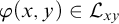 $\varphi (x,y) \in \mathcal {L}_{xy}$
and
 $d \in \mathcal {U}^{y}$
. Consider

We provide the following justifications:
-
(a) Since
and
$\mathbb {E}[\varphi (x,f_{d})] \in \mathcal {L}_{x}^{R}(\mathcal {U}^{\Omega })$
. -
(b) Proposition 2.9.
 and

Theorem 3.3 (T NIP).
Suppose
 $\mu \in \mathfrak {M}_{x}^{\mathrm {fs}}(\mathcal {U},M)$
and
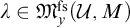 $\lambda \in \mathfrak {M}_{y}^{\mathrm {fs}}(\mathcal {U},M)$
. Then
 $s_{\mu } \otimes s_{\lambda } = s_{\mu \otimes \lambda }$
.
Proof. Fix
 $\varphi (x,y,z) \in \mathcal {L}_{xyz}$
and
 . Let
 . Now consider the following computation:

We provide the following justifications:
-
(a) We show
. Indeed, if
$\varphi (y,z,w) \in \mathcal {L}_{yzw}$
and
$a \in M^{w}$
, then We provide the following mini-justifications:
-
(i) Proposition 3.2.
-
(ii) This is an instance of currying. Consider the map
$\rho _{a} :S_{z}(M) \to S_{zw}(M)$
where
$\rho _{a}(q)$
is the unique type in
$S_{zw}(M)$
such that
$\rho (q)|_{z} = q$
and
$\rho (q)|_{w} = \operatorname {tp}(a/M)$
. Then if we let
$(\rho _a)_*$
denote the push-forward from
$\mathfrak {M}_{z}(M)$
to
$\mathfrak {M}_{zw}(M)$
, we see that Then for any
$\theta (x) \in \mathcal {L}_{zw}(M)$
, -
(iii) Proposition 3.1.
-
(iv) Since
.
-
-
(b) Proposition 3.2.
-
(c) Associativity of the Morley product in NIP theories.
 . Indeed, if











 .
Remark 3.4. Theorem 3.3 and along with Proposition 2.2 give another proof of the following: Suppose that
 $\mu \in \mathfrak {M}_{x}^{\mathrm {inv}}(\mathcal {U},M)$
,
 $\nu \in \mathfrak {M}_{x}^{\mathrm {inv}}(\mathcal {U},M)$
, and both
 $\mu $
and
 $\nu $
are definable. Then
 $$ \begin{align*} r_{\mu}(x) \otimes r_{\nu}(y) = r_{\mu \otimes \nu}(x,y). \end{align*} $$
This was originally proved in [Reference Conant, Gannon and Hanson18, Proposition 3.15]. The only difference in the proof is the justification of
 $(c)$
. Here “associativity of the Morley product in NIP theories” is replaced by “associativity of the Morley product for definable measures in arbitrary theories” (see Remark 1.5).
Remark 3.5. If the types
 $\{s_{\mu } : \mu \in \mathfrak {M}_{x}^{\mathrm {inv}}(\mathcal {U},M)\}$
are consistent, then the proof of Theorem 3.3 directly generalizes to this case as well.
4 Going down: The restriction map and the Morley product
We warn the reader that the restriction map does not interact well with arbitrary Morley products.
Warning . We remark that, in general,
 $\nu _{p} \otimes \nu _{q} \neq \nu _{p \otimes q}$
. Fix any
 $A \subseteq \Omega _0$
such that
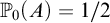 $\mathbb {P}_0(A) = 1/2$
and
 $b_1,b_2 \in M$
. Consider the random elements
 $g_1,g_2:\Omega \to \mathcal {U}$
where
 $$ \begin{align*} g_1(t)=\begin{cases} \begin{array}{@{}cc} b_{1} & t\in A,\\ b_{2} & t\in A^{c}, \end{array}\end{cases} \text{and } g_2(t)=\begin{cases} \begin{array}{@{}cc} b_{2} & t\in A,\\ b_{1} & t\in A^{c}. \end{array}\end{cases} \end{align*} $$
Let  and
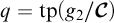 :
 $$ \begin{align*} \nu_{p \otimes q}(x = y) = 0 \text{ and } (\nu_{p} \otimes \nu_{q}) (x = y) = 1/2. \end{align*} $$
This warning shows us that we cannot expect
 $\nu _{p \otimes q} = \nu _{p} \otimes \nu _{q}$
. However, we would like a condition which implies that the Morley product commutes with the restriction map. It turns out that one can give a characterization of this property, for finitely satisfiable types, by writing down a family of equalities. This condition is a kind of strong probabilistic independence which we call prob. independence. We then prove that in the NIP setting, p is prob. independent over q if and only if
 $\nu _{p \otimes q} = \nu _{p} \otimes \nu _{q}$
.
Definition 4.1 (Prob. independence).
Let
 $h \in (\mathcal {U}_0^{\Omega })^{x}$
and
 . We say that h is prob. independent over b if for any partition
 $\mathcal {A}$
for h,
 $\mathcal {L}$
-formulas
 $\theta (x,y,z)$
, and points
 $e \in \mathcal {U}^{z}$
, we have that
 $$ \begin{align*} \mathbb{E}[\theta(h,b,f_{e})] = \sum_{A \in \mathcal{A}} \mathbb{P}_0(A) \mathbb{E}[\theta(f_{h|_A},b,f_{e})]. \end{align*} $$
If  , we say that p is prob. independent over b if there exists a net
 $(h_i)_{i \in I}$
of points in
 $M_{0}^{\Omega }$
such that
 , and for any
 $\mathcal {L}$
-formula
 $\theta (x,y,z)$
and parameters e from
 $\mathcal {U}^{z}$
,
 $$ \begin{align*} \mathbb{E}[\theta(x,b,f_{e})]^{p} = \lim_{i \in I} \sum_{A \in \mathcal{A}_i} \mathbb{P}_0(A)\mathbb{E}[\theta(f_{h_i|_A},b,f_e)], \end{align*} $$
where
 $\mathcal {A}_i$
is a partition for
 $h_i$
.
Finally, we say that a type  is prob. independent over a type
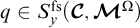 if for some/any
 we have that p is prob. independent over b.
We now give three examples of different kinds of random variables which satisfy the condition above. Our first example deals with constant random variables, the second with extensions-by-definition, and the final one is constructed by hand.
Fact 4.2. For any
 $e \in M$
and
 , we have that:
-
(1)
$f_e$
is prob. independent over b. -
(2)
is prob. independent over b. -
(3) For any
$a \in M$
, is prob. independent over .

 is prob. independent over b.

 is prob. independent over
 .
Proposition 4.3 (T NIP).
If
 $\mu \in \mathfrak {M}_{x}^{\mathrm {fs}}(\mathcal {U},M)$
and
 , then
 $s_{\mu }$
is prob. independent over b. This implies that for any
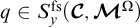 ,
 $s_{\mu }$
is prob. independent over q.
Proof. By Proposition 2.4, we know that
 $s_{\mu }$
is finitely satisfiable in
 and so the proposition itself makes sense. Fix an
 $\mathcal {L}$
-formula
 $\varphi (x,y,z)$
, parameters
 $e \in \mathcal {U}^{z}$
, and a net
 $(h_i)_{i \in I}$
such that
 . For each
 $i \in I$
, we let
 $\mathcal {A}_i$
be a partition for
 $h_i$
. Notice that
 because

where the first equality follows from Proposition 2.9 and the last equality follows from continuity of
 $\nu _{-}$
(Proposition 1.3). Now we compute

We remark that Equation
 $(*)$
follows from left-continuity of the Morley product in NIP theories (see Remark 1.5). Equation
 $(**)$
is just Fact 2.1.
We now given an example of a type and a point in  such that the type is not prob. independent over all points in
 . Hence the results in this section are not just about extensions-by-definition.
Example 4.4. Consider  and the partition
 $\mathcal {A} =\{A_1,A_2,A_3,A_4\}$
where:
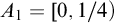
-
•
$A_1 = [0,1/4)$
. -
•
$A_2 = [1/4,1/2)$
. -
•
$A_3 = [1/2,3/4)$
. -
•
$A_4 = [3/4, 1]$
.



Let
 $a,b,c \in M$
and consider the elements
 $$ \begin{align*} g_1(t)=\begin{cases} \begin{array}{@{}cc} a & t\in A_1 \cup A_2,\\ b & t\in A_3 \cup A_4. \end{array}\end{cases} g_2(t)=\begin{cases} \begin{array}{@{}cc} a & t\in A_1 \cup A_3,\\ b & t\in A_2 \cup A_4. \end{array}\end{cases} g_3(t)=\begin{cases} \begin{array}{@{}cc} a & t\in A_1 \cup A_2,\\ c & t\in A_3 \cup A_4. \end{array}\end{cases} \end{align*} $$
We claim that the type  is prob. independent over
 $g_2$
, but
 is not prob. independent over
 $g_3$
. We leave this as an exercise.
Proposition 4.5 (T NIP).
If  ,
 and p is prob. independent over q, then
 $\nu _{p \otimes q} = \nu _{p} \otimes \nu _{q}$
.
Proof. Since p is prob. independent over q, there exists a net
 $(h_i)_{i \in I}$
of elements in
 $M_0^{\Omega }$
witnessing this property. For each
 $i \in I$
, we let
 $\mathcal {A}_i$
be a partition for
 $h_i$
. Let
 . Fix an
 $\mathcal {L}$
-formula
 $\varphi (x,y,z)$
and a tuple of parameters
 $e \in \mathcal {U}^{z}$
. Now consider the following computation:

We provide the following justifications:
-
(a) Hypothesis on choice of
$(h_i)_{i \in I}$
, i.e., witnessing prob. independence. -
(b) Easier to see from bottom to top; direct computation from the fact that the measure on the left-hand side of the Morley product is a weighted sum of Dirac measures concentrating on realized types.
-
(c) In NIP, the map
$-\otimes \lambda (\psi (x,y))$
is continuous and thus commutes with nets (see Remark 1.5). -
(d) Reverse direction of Fact 2.1.
-
(e) Continuity of the map
$\nu _{-}$
(Proposition 1.3). -
(f) Straightforward to check that
. Similar to Proposition 3.2.



 . Similar to Proposition
We now prove the main result of this section.
Theorem 4.6 (T NIP).
Suppose  and
 . Then any net from
 $M_{0}^{\Omega }$
which converges to p witnesses the fact that p is prob. independent over q. More precisely, the following are equivalent:
-
(1) p is prob. independent over q.
-
(2)
$\nu _{p \otimes q} = \nu _{p} \otimes \nu _{q}$
. -
(3) For any
$\mathcal {L}$
-formula
$\varphi (x,y,z)$
and any
$e \in \mathcal {U}^{z}$
, for any
$(h_i,\mathcal {A}_i)_{i \in I}$
such that
$h_i \in M_{0}^{\Omega }$
,
$\mathcal {A}_i$
is a partition for
$h_i$
and ,
$$ \begin{align*} \lim_{i \in I} \sum_{A \in \mathcal{A}_i} \mathbb{P}(A) (\mathbb{E}[\varphi(f_{h_i|_{A}},y,f_{e})])^{q} = (\mathbb{E}[\varphi(x,y,f_{e})])^{p \otimes q}. \end{align*} $$



 ,

Proof.
 $(1) \Rightarrow (2)$
is Proposition 4.5.
 $(3) \Rightarrow (1)$
is trivial. Indeed, we are only swapping for all and there exists. We prove
 $(2) \Rightarrow (3)$
. Fix a formula
 $\varphi (x,y,z)$
, a sequence
 $(h_i,A_i)_{i \in I}$
with the relevant properties, and an element
 $e \in \mathcal {U}^{z}$
. Then

Many of the justifications are similar to the previous direction. We leave this as an exercise to the reader.
Corollary 4.7 (T NIP).
Suppose that
 $\mu \in \mathfrak {M}_{x}^{\mathrm {fs}}(\mathcal {U},M)$
and
 . Then
 $\nu _{(s_{\mu } \otimes p)} = \mu \otimes \nu _{p}$
.
Proof. Follows directly from the fact that
 $s_{\mu }$
is prob. independent over every type, the previous proposition, and Fact 2.9.
Remark 4.8. In practice, it is quite difficult to compute the Morley product when there are non-trivial dependencies around. Even in the case where one of the types is realized and the other is an extension-by-definition. We consider the following computation: Let
 $h \in (M_{0}^{\Omega })^{y}$
with partition
 $\mathcal {A}$
,
 ,
 $\mu \in \mathfrak {M}_{x}^{\mathrm {inv}}(\mathcal {U},M)$
, where
 $\mu $
is Borel-definable, and
 $\varphi (x,y,z)$
be an
 $\mathcal {L}$
-formula. Then we have that

We prove the following justifications:
-
(a) If
$\theta (x,y) = \bigvee _{A \in \mathcal {A}} y =h|_{A}$
, then . The sets
$\{[y_i = h|_{A}]\}_{A \in \mathcal {A}}$
form a partition of (see Lemma 5.4). -
(b) For notational purposes, we let
. -
(c) Notice that if
$r \in \mathrm {supp}(\frac {1}{\mathbb {P}_0(A)} \lambda _{A})$
and
$(c,d) \models r(y,z)$
, then
$c = h|_{A}$
. -
(d) Standard push-forward technique.

 . The sets

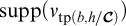 (see Lemma
 .



The most complicated portion of the term above is the measure we are integrating with respect to,
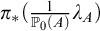 $\pi _{*}(\frac {1}{\mathbb {P}_0(A)} \lambda _{A})$
. We remark that in the case where h is prob. independent over b, it is straightforward to check that
 , and the computation continues, resulting in
 $(\mathbb {E}[\varphi (x,y,b)])^{s_{(\mu \otimes \nu _{p})}}$
. In the general case, it seems like this term needs to be considered on a case-by-case basis, or one needs to know more information about the fiber function,
 $F_{\mu }^{\varphi }$
.
Finally, we observe that if p is prob. independent over q, then the realizations of these types, as random elements, are stochastically independent. Consider the following definition.
Definition 4.9. Suppose that  and
 . Consider
 where
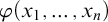
 . By [Reference Andrews, Goldbring and Keisler1, Proposition 2.1.10] (see also [Reference Ben Yaacov5, Theorem 3.11]), the model
 is isomorphic to a reduction of a nice randomization of a model
 $\mathcal {N}'$
(of T). In particular, we have that
-
(1)
. -
(2)
is a atomless probability algebra. -
(3)
is a collection of functions from to
$\mathcal {N}'$
. -
(4) For every
$\mathcal {L}$
-formula
$\varphi (x_1,\ldots ,x_n)$
and tuple
$b_1,\ldots ,b_n$
from , we have that -
(5)
.
 .
 is a atomless probability algebra.
 is a collection of functions from
 to



 , we have that

 .
For any
 $\mathcal {L}$
-formula
 $\varphi (x,y)$
,
 $e \in \mathcal {U}^{y}$
, and
 , we let

For any  we let

Finally, we say that the types p and q stochastically independent if whenever  ,
 $a \models p,$
and
 $b \models q$
, then
 .
Proposition 4.10. Let  and
 . If p is prob. independent over q, then p and q are stochastically independent.
Proof. We prove by contraposition. Suppose that p is not stochastically independent over q. Then there exists some non-trivial  where
 $a \models p$
and
 $b \models q$
. Then there exist
 $\mathcal {L}(\mathcal {U})$
-formulas
 $\varphi _1(x,e_1)$
and
 $\varphi _2(x,e_2)$
such that

and,

Now notice that

However,

Since  , we have that
 . Hence
 and so
 $\nu _{p \otimes q} \neq \nu _{p} \otimes \nu _{q}$
.
5 Ellis semigroup of randomization
In this last section, we make some comments concerning the Ellis semigroup of the randomization. We show that the map
 $s_{-}$
is an injective embedding from the convolution algebra of Keisler measures to the semigroup of types over the randomization (under the Newelski product). We then show that if our group is definably amenable, then any minimal left ideal of the Ellis semigroup of finitely satisfiable types is a single point. Finally, we observe that if our group is not definably amenable, then the minimal left ideals of
 are more complicated than the minimal left ideals of
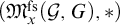 $(\mathfrak {M}^{\mathrm {fs}}_{x}(\mathcal {G},G),*)$
. We recall the standard set up as follows.
Definition 5.1. Let T be a first-order theory expanding a group. Let
 $G \models T$
and
 $\mathcal {G}$
be a monster model such that
 $G \prec \mathcal {G}$
. Again,
 . We recall the construction of the Newelski product: Given
 , any
 $\mathcal {L}$
-formula
 $\varphi (x,z)$
, and
 , we have that
 $$ \begin{align*} (\mathbb{E}[\varphi(x,b)])^{p*q} = (\mathbb{E}[\varphi(x \cdot y,b)])^{p\otimes q}. \end{align*} $$
We remark that if  , then
 .
We now quickly recall the definition of definable convolution.
Definition 5.2 (T is NIP).
Fix
 $\mu ,\nu \in \mathfrak {M}_{x}^{\mathrm {fs}}(\mathcal {G},G)$
. The convolution product of
 $\mu $
and
 $\nu $
is the unique measure
 $\mu * \nu $
in
 $\mathfrak {M}_{x}^{\mathrm {fs}}(\mathcal {G},G)$
such that for any
 $\mathcal {L}$
-formula
 $\varphi (x,z)$
and parameter
 $d \in \mathcal {G}^{z}$
, we have that
 $$ \begin{align*} (\mu * \nu)(\varphi(x,d)) = (\mu_{x} \otimes \nu_{y})(\varphi(x \cdot y,d)). \end{align*} $$
We recall that if
 $\mu ,\nu \in \mathfrak {M}_{x}^{\mathrm {fs}}(\mathcal {G},G)$
, then
 $\mu * \nu \in \mathfrak {M}_{x}^{\mathrm {fs}}(\mathcal {G},G)$
.
Proposition 5.3 (T NIP).
The map  is an injective embedding of semigroups.
Proof. The map
 $s_{-}$
is continuous by Proposition 2.5 and injective since for any
 $\mathcal {L}$
-formula
 $\varphi (x,y)$
and
 $b \in \mathcal {U}$
,
 $(\mathbb {E}[\varphi (x,f_{b})])^{s_\mu } = \mu (\varphi (x,b))$
. We show that our map is a homomorphism. Fix an
 $\mathcal {L}$
-formula
 $\varphi (x,z)$
. Let
 $\varphi '(x;y,z) = \varphi (x \cdot y, z)$
and fix
 . Now notice that

where Equation
 $(*)$
holds from Theorem 3.3. By quantifier elimination, the statement holds.
Our next proposition shows that if G is NIP definably amenable, then any minimal left ideal of  is a single point. This observation is an extension of [Reference Berenstein and Muñoz8, Proposition 4.18]—if an NIP group G is definably amenable, then
 $G^{\Omega }$
is extremely definably amenable. The general idea of the argument is similar and our proof relies on this work modified to the appropriate setting. We also remark that this statement is known outside of the NIP case (i.e., if G is definably amenable, then
 $G^{\Omega }$
is extremely definably amenable [Reference Carmona and Onshuus9, Theorem 6.3]).
Lemma 5.4. Suppose that
 $h \in (M^{\Omega }_0)^{y}$
and
 . Let
 $\mathcal {A}$
be a partition for h. Then for every
 , if
 $(a,c) \models r(y,z)$
then there exists some
 $A \in \mathcal {A}$
such that
 $a = h|_{A}$
.
Proof. By Fact 2.1,  . Let
 $\theta (y) : = \bigvee _{A \in \mathcal {A}} (y = h|_{A})$
. Notice that

Since the set
 $\theta (y) \wedge z=z$
has measure 1, it follows that every type in the support of
 contains the formula
 $\theta (y) \wedge x =x$
. This implies the intended result.
Proposition 5.5 (T NIP).
Suppose that G is definably amenable. Fix
 $\mu \in \mathfrak {M}_{x}^{\mathrm {fs}}(\mathcal {G},G)$
such that
 $\mu $
is left-G-invariant (these exist by [Reference Chernikov, Pillay and Simon13, Theorem 3.17]). Then for any
 we have that
 $$ \begin{align*} p * s_{\mu} = s_{\mu}. \end{align*} $$
Thus
 $\{s_{\mu }\}$
is a minimal left ideal. As a consequence
 $s_{\mu }|_{G^{\Omega }}$
is left-
 $G^{\Omega }$
-invariant which implies that
 $G^{\Omega }$
is extremely definably amenable.
Proof. Fix an
 $\mathcal {L}$
-formula
 $\varphi (x,z)$
and an element
 . Choose
 $(h_i)_{i \in I}$
such that
 $h_i \in M_0^{\Omega }$
and
 . Let
 $\varphi ^{+}(x;y,z) := \varphi (y \cdot x, z)$
. Let
 $\pi _{z}$
denote the standard projection map from
 $S_{yz}(M) \to S_{z}(M)$
and
 $(\pi _{z})_*: \mathfrak {M}_{yz}(M) \to \mathfrak {M}_{z}(M)$
be the corresponding push-forward map. Then

We justify Equation
 $(*)$
. Notice that if
 and
 $(a,c) \models r$
then
 $a \in G$
by Lemma 5.4. Notice that since
 $\mu $
is left-G-invariant, we have
 $$ \begin{align*} F_{\mu}^{\varphi^{+}}(r) = \mu(\varphi(a \cdot x, b)) = \mu(\varphi(x, b)) = \left(F_{\mu}^{\varphi} \circ \pi_{z}\right) (r).\\[-34pt] \end{align*} $$
The following proposition is a sanity check.
Proposition 5.6. Suppose that any minimal left ideal of  is a singleton. Then G is definably amenable.
Proof. Suppose there exists some  such that for any
 ,
 $p * q = q$
. This implies that
 $\nu _{q}|_{G}$
is left-G-invariant since for any
 $g \in G$
and
 $\theta (x) \in \mathcal {L}_{x}(G)$
,

Thus G is definably amenable.
Our final proposition demonstrates that if G is not definably amenable, then the minimal left ideal of  is not
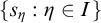 $\{s_{\eta }: \eta \in I\}$
where I is a minimal left ideal in
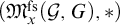 $(\mathfrak {M}_{x}^{\mathrm {fs}}(\mathcal {G},G),*)$
. To be honest, I thought it was going to work out nicely and
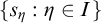 $\{s_{\eta }:\eta \in I\}$
would be a minimal left ideal. As they say, you win some, you lose some.
Proposition 5.7 (T NIP).
Suppose that G is not definably amenable. Let
 $I \subseteq (\mathfrak {M}_{x}^{\mathrm {fs}}(\mathcal {G},G),*)$
be a minimal left ideal. Then
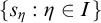 $\{s_{\eta }: \eta \in I\}$
is not a left ideal of
 .
Proof. We recall from [Reference Chernikov and Gannon11] that I is a compact convex set. Fix
 $\mu \in I$
such that
 $\mu $
is an extreme point, i.e., for any distinct
 $\lambda _1,\lambda _2 \in I$
and
 $t \in (0,1)$
,
 $$ \begin{align*} \mu \neq t\lambda_1 + (1-t)\lambda_2. \end{align*} $$
We recall that extreme points exist by the Krein–Milman theorem. Since G is not definably amenable, there exists
 $g \in G$
such that
 $\mu _{g} \neq \mu $
, where
 $\mu _{g}$
is the left translate of
 $\mu $
by g. Now notice that
 $$ \begin{align*} \mu \neq \frac{1}{2}\mu_{g^{-1}} + \frac{1}{2} \mu_{g}, \end{align*} $$
since
 $\mu $
is extreme. Thus there exists an
 $\mathcal {L}$
-formula
 $\theta (x,y)$
and some
 $b \in \mathcal {U}$
such that
 $$ \begin{align*} \mu(\theta(x,b)) \neq \left( \frac{1}{2}\mu_{g^{-1}} + \frac{1}{2}\mu_{g} \right)(\theta(x,b)). \end{align*} $$
Now fix
 $A \subseteq \Omega _0$
such that
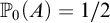 $\mathbb {P}_0(A) = 1/2$
and consider the random element
 $$ \begin{align*} h(t)=\begin{cases} \begin{array}{@{}cc} g & t\in A,\\ e & t\in A^{c}. \end{array}\end{cases} \end{align*} $$
Now suppose that
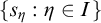 $\{s_{\eta } : \eta \in I\}$
is a minimal left ideal. Then there exists some
 $\lambda \in I$
such that
 . But this is impossible. The simplest way to see this is via an automorphism argument. Consider an automorphism
 $\sigma $
of
 $\mathcal {B}_0$
which sends A to
 $A^{c}$
. We can extend this automorphism to an automorphism of the randomization which fixes all constant random variables from
 $\mathcal {G}^{\Omega }$
. We claim that the type
 $s_{\lambda }$
is fixed under this automorphism while
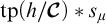 is not. Indeed, we first see that
 $s_{\lambda }$
is invariant. Fix a parameter
 . Notice that
 because for any
 $\mathcal {L}$
-formula
 $\theta (y,z)$
and parameter
 $d \in M^{z}$
,

Now for any
 $\mathcal {L}$
-formula
 $\psi (x,y)$
,

since the integration is (formally) occurring with respect to the measures  and
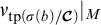 . Hence
 $s_{\lambda }$
is fixed under this automorphism.
We now argue that 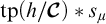 is not invariant. Consider the elements
 $$ \begin{align*} f(t)=\begin{cases} \begin{array}{@{}cc} e & t\in A,\\ g_1^{-1} & t\in A^{c}. \end{array}\end{cases} \text{and } k(t) =(f\cdot h) (t)=\begin{cases} \begin{array}{@{}cc} g & t\in A,\\ g_1^{-1} & t\in A^{c}. \end{array}\end{cases} \end{align*} $$
Then if
 $\varphi ^{+}(x;yz) = \varphi (y \cdot x,z)$
,

Funding
K.G. was supported by the Fundamental Research Funds for the Central Universities, Peking University (Grant No. 7100604835) and by the National Natural Science Fund of China (Grant No. 12501001).
Acknowledgments
The author thanks Itaï Ben Yaacov for discussions. The author is also deeply indebted to James Hanson for shaping his intuition about the subject. The author thanks the anonymous referee for many helpful comments.


