1 Introduction
The interaction between the wake of an upstream body and the boundary layer developing on the surface of a downstream body is often encountered in engineering applications, such as the multi-element airfoils, turbo-machinery and pipelines near the ground (Squire Reference Squire1989; Sarkar & Sarkar Reference Sarkar and Sarkar2010). The downstream body is affected by the wake characterized by a loss of total pressure and increase in turbulence level. Moreover, there may be large coherent vortices in the wake which can completely change the flow pattern and the forces acting on the bodies.
Such wake/boundary layer interaction can be investigated using a simplified model with a two-dimensional circular cylinder transversely placed above a flat plate. Bearman & Zdravkovich (Reference Bearman and Zdravkovich1978) experimentally investigated the flow around the circular cylinder placed at various heights above a flat plate. Hot-wire surveys were conducted at Reynolds number
 $Re_{D}$
, based on the cylinder diameter, of
 $2.5\times 10^{4}$
. Distributions of mean pressure around the cylinder and along the plate were measured at
 $Re_{D}=4.5\times 10^{4}$
. Hot-wire signals demonstrated that lower wake vortex shedding was suppressed for all gaps less than approximately
 $G/D=0.3$
, while above this critical value, regular wake vortex shedding was restored. The presence of the wall has an impact on the pressure distribution. For
 $G/D=0$
and 0.1 the pressure distributions around the cylinder was asymmetric. For
 $G/D=0.4$
and 0.8 the pressure distributions became nearly symmetric, however, the symmetric axis was not in the free-stream direction but rotated in the counter-clockwise direction, suggesting the downward movement of the front stagnation point on the cylinder. As to the pressure distribution on the plate, due to the effects of the gap flow, there was a rapid fall in pressure below the cylinder and the minimum value was recorded just behind the gap. When
 $G/D$
was further increased the pressure distribution on the cylinder assumed a symmetrical form with the axis of symmetry approaching the free-stream direction. Flow visualizations in a smoke tunnel revealed the flow structures at various
 $G/D$
ratios, including the wake vortex shedding at higher gap ratios and the separation bubbles both upstream and downstream of the cylinder at small gap ratios.
Price et al. (Reference Price, Sumner, Smith, Leong and Paidoussis2002) visualized the fluid flow around a circular cylinder near to a plane wall for Reynolds numbers
 $Re_{D}$
between 1200 and 4960. The gap height ranged from
 $G/D=0$
to
 $G/D=2.0$
and four distinct regions were identified for describing the observed flow dynamics. For
 $G/D\leqslant 0.125$
, the gap flow was either suppressed or extremely weak, and no regular vortex shedding occurred downstream of the cylinder. However, it was possible to detect a periodicity in the upper shear layer of the cylinder. Separation of the boundary layer occurred both upstream and downstream of the cylinder. For
 $0.125<G/D<0.5$
, the flow was very similar to the previous region, except that there was a pronounced pairing between the lower shear layer shed from the cylinder and the wall boundary layer. For
 $0.5<G/D<0.75$
, it was characterized by the onset of vortex shedding from the cylinder. For the fourth region, characterized by the largest gap ratios considered,
 $G/D>1.0$
, there was no separation of the wall boundary layer, either upstream or downstream of the cylinder. In addition, the flow around the cylinder was essentially the same as the flow around an isolated circular cylinder.
Sarkar & Sarkar (Reference Sarkar and Sarkar2009, Reference Sarkar and Sarkar2010) numerically investigated flow past a circular cylinder placed near a wall at
 $Re_{D}=1440$
using large eddy simulations (LES). The LES revealed that the
 $G/D$
ratio has a strong influence on shear layer instability, the modification of wake dynamics and turbulence characteristics. When the lower shear layer from the cylinder was inside the boundary layer (
 $G<\unicode[STIX]{x1D6FF}$
,
 $\unicode[STIX]{x1D6FF}$
is the local boundary layer thickness), a strong coupling between the inner shear layer and the approaching boundary layer was observed, with suppression of the vortex shedding and stretching of the shear layers. The boundary layer was deflected from the wall, resulting in a large separation. The mutual interactions of the wall vortices with the shed vortices caused the trajectories of the shed vortices to cross each other, leading to an inversion on the position of the vortices with respect to the unbounded case. Turbulence was mainly generated in the wake and the near-wall region was relatively calm. When the cylinder was kept outside of the boundary layer (
 $G=2.4\unicode[STIX]{x1D6FF}$
), the shear layers and the boundary layer can be separately identified. The vortices shed from the cylinder can disturb the boundary layer during their convection, triggering its transition, and the amplification of the turbulent stresses in this case was found near the wall.
The vortex shedding frequency and forces on the cylinder can be altered in the proximity of a wall. Most studies in the literature reported that, as long as regular vortex shedding occurred, the Strouhal number
 $St$
remained constant with respect to the varying gap ratio (Bearman & Zdravkovich Reference Bearman and Zdravkovich1978; Zdravkovich Reference Zdravkovich1985; Taniguchi & Miyakoshi Reference Taniguchi and Miyakoshi1990). The Reynolds number in these studies was usually over
 $10^{4}$
. Angrilli, Bergamaschi and Cossalter (Reference Angrilli, Bergamaschi and Cossalter1982) investigated the effect of
 $G/D$
on the vortex shedding frequency in a much lower range of
 $Re_{D}$
(2860, 3820 and 7640). They found that
 $St$
increased when the cylinder approached the wall. Angrilli et al. (Reference Angrilli, Bergamaschi and Cossalter1982) claimed that the different responses of
 $St$
with respect to gap ratio were due to the differences in
 $Re_{D}$
. This has been confirmed by the study of Price et al. (Reference Price, Sumner, Smith, Leong and Paidoussis2002), who found that for low Reynolds number flows,
 $Re_{D}<2600$
, the Strouhal number for small gap ratios was significantly greater than that for an isolated circular cylinder. For higher Reynolds numbers (
 $Re_{D}>4000$
), however,
 $St$
seems to be insensitive to
 $G/D$
. As stated earlier, the approach of the cylinder to the wall caused the downstream movement of the frontal stagnation point towards the wall, which produced an upward lift. In the meantime, the base pressure of the cylinder increased, resulting in a decreased drag coefficient. Taniguchi & Miyakoshi (Reference Taniguchi and Miyakoshi1990) and Lei, Cheng & Kavanagh (Reference Lei, Cheng and Kavanagh1999) observed that when the lower surface of the cylinder was placed within the critical gap ratio, the fluctuations of both lift and drag coefficients could be strongly reduced.
Aside from the above research, which focused on gap ratio effects on the wake flow pattern and the forces on the circular cylinder, some studies in the literature have paid more attention to the transition of the flat plat boundary layer under the influence of the wake perturbations. The visualization study of Pan et al. (Reference Pan, Wang, Zhang and Feng2008) at
 $Re_{D}=2000$
revealed that spanwise secondary vortices were periodically induced by the passing wake vortices. The transition of the boundary layer featured downstream evolution of these secondary vortices into
 $\unicode[STIX]{x1D6EC}$
/hairpin vortices. The primary hairpin vortices then generated new hairpin vortices upstream, leading to the formation of streamwise elongated hairpin packets which were populated in the final turbulent boundary layer. The presence and the evolution of the secondary vortices were later confirmed by the experimental study of Mandal & Dey (Reference Mandal and Dey2011) with particle image velocimetry at
 $Re_{D}$
between 929 and 3310. Mandal & Dey (Reference Mandal and Dey2011) concluded that although the nature of disturbances in wake-induced boundary layer transition is different from that in a free-stream-turbulence (FST)-induced transition, the late stage process seemed to be the same in both transition scenarios. He et al. (Reference He, Wang and Pan2013) investigated the initial growth of disturbances associated with the evolution of secondary vortices in the boundary layer. Recently, He et al. (Reference He, Pan, Feng, Gao and Wang2016) revealed the Lagrangian coherent structures (LCS) in the wake-disturbed boundary layer using the finite time Lyapunov exponents (FTLE) method. Statistics of the LCS, including the wall-normal profiles of the mean convection velocity and the averaged inclination angle, were presented for the first time.
Vortices are the ‘sinews and muscles of fluid motions’ (Kuchemann Reference Küchemann1965). The investigation of vortices and their interactions are crucially important because of the observed existence of coherent vortical structures in many types of turbulent flows, such as jets, wakes, mixing layers and boundary layers. Representing turbulence as a superposition of interacting vortices may be a valid and useful idea (Saffman & Baker Reference Saffman and Baker1979). Great effort has been made to investigate the generation, motion, evolution, instability and decay of vortices in various types of flows (see Roshko (Reference Roshko1976), Williamson (Reference Williamson1996) and Smith & Glezer (Reference Smith and Glezer1998) for a few examples) and the research has remained active after many years. The investigation of interactions among vortices or between vortices and solid bodies are even more challenging because of the nonlinearity which is present in most cases. Existing studies on vortex interactions often rely on theoretical computation of the instability of vortices with given sizes, spatial arrangement and usually the assumption that the external forcing or perturbation acting on the vortices is not strong (Saffman & Baker Reference Saffman and Baker1979; Saffman Reference Saffman1981; Doligalski Reference Doligalski1994; Dritschel Reference Dritschel1995). Progress has been made, but much remains to be learned about the interactions of vortices, especially when strong nonlinearity sets in.
There have been many studies on the flow past a cylinder in proximity to a wall and the effects of gap ratios have been discussed, as shown above. However, most of the previous studies are based on mean statistics from pressure taps and hot-wires. The investigations of vortex dynamics, especially the complex vortex interaction phenomenon, is scarce. The vortex dynamics is however of great importance to the understanding of the flow phenomena and mechanism. Therefore, the present research aims at investigating the vortex dynamics in the cylinder wake/wall boundary layer interactions at various gap ratios. The vortex formation and evolution process will be discussed. Moreover, the vortex interaction and the breakdown process will be investigated in detail. It is hoped that this study on vortex dynamics can shed some light on the flow physics and help to elucidate the characteristics of mean statistics.
2 Experimental set-up
The experimental set-up has already been described in a previous work of the authors, so here we just give a brief introduction and one can refer to He et al. (Reference He, Pan, Feng, Gao and Wang2016) for more details. The low-speed water tunnel where the experiment was conducted had a working section of
 $600~\text{mm}\times 600~\text{mm}\times 3000~\text{mm}$
(height
 $\times$
width
 $\times$
length). The incoming free-stream velocity
 $U_{\infty }$
at the inlet of the working section was
 $67~\text{mm}~\text{s}^{-1}$
with a turbulence intensity
 $Tu$
less than
 $0.8\,\%U_{\infty }$
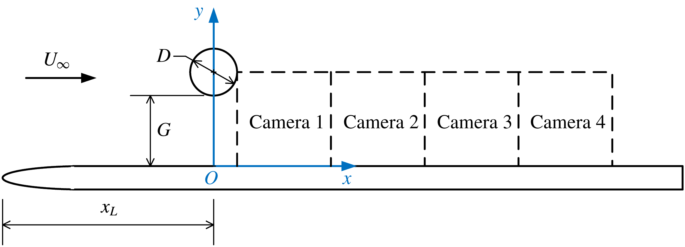
. The experimental schematic and the coordinates definition are illustrated in figure 1. A circular cylinder was placed above a flat plate with its axis parallel to the leading edge of the plate. The diameter
 $D$
of the circular cylinder was 20 mm. The Reynolds number based on the cylinder diameter
 $Re_{D}=U_{\infty }D/\unicode[STIX]{x1D708}$
was 1072 and the Strouhal number
 $St=f_{0}D/U_{\infty }$
was 0.21. The flat plate boundary layer, without the presence of the cylinder, was laminar and had a thickness
 $\unicode[STIX]{x1D6FF}$
of 10.6 mm (
 $\unicode[STIX]{x1D6FF}/D=0.53$
) at the location of the cylinder. The investigated gap heights
 $G$
between the cylinder and the flat plate were 0 mm, 5 mm, 10 mm, 20 mm, 30 mm, 40 mm, 50 mm and 60 mm, corresponding to a
 $G/D$
ratio from 0 to 3.0.
The flow field was measured by a two-dimensional particle image velocimetry system. The measurements were conducted in the streamwise plane perpendicular to wall (side view) at the middle of the cylinder. The particle images were recorded at a frequency 100 Hz by four charge-coupled device (CCD) cameras which were aligned in the streamwise direction (see figure 1). Multi-pass interrogation algorithm was used to analyse the particle images with the final interrogation window size of
 $16\times 8$
pixels and a 50 % overlap. The uncertainty of the measured velocity was estimated to be less than
 $2\,\%U_{\infty }$
. The total sampling duration was more than 3 min and a total number of 19 050 image frames were recorded.
Experimental set-up and coordinates definition.

3 Virtual dye visualization
Dye visualization is a common experimental technique which is widely used to reveal flow structures in fluid flow. Use of the technique has resulted in substantial contributions to the studies of fluid mechanics in various fields, such as wakes, mixing layers and boundary layers etc. It relies on the light reflected from the physical particles seeded in the transparent fluid to reveal the coherent structures in the flow. Although this technique is effective and easy to implement, there are several limitations. Firstly, the dye (such as ink or hydrogen bubbles in water and smoke in the air) may suffer from diffusion and can only be visualized in a limited range of the flow, especially in turbulent flows. Secondly, the dye is usually monochrome and a chromatic visualization either increases the complexity of the experiments or is utterly impossible (such as hydrogen bubble visualization). Finally, the physical particles seeded in the flow have to be small enough to accurately follow the flow. In the present study, virtual dye visualization based on quantitative PIV data is used instead.
The principle of virtual dye visualization is simple. Virtual tracers are released from a certain location and allowed to advect with the flow, revealing the nearby coherent structures. If the virtual tracers are released from different locations, they can be easily tagged with different colours according to their initial positions, therefore the interactions of different coherent structures can be revealed in detail. Like dye visualization in real experiments, the virtual dye visualizes the attracting LCS in the flow. Virtual tracers have been used before to reveal fluid transport in vortex formation (Shadden et al. Reference Shadden, Katija, Rosenfeld, Marsden and Dabiri2007) and in the feeding process of a jellyfish (Shadden, Dabiri & Marsden Reference Shadden, Dabiri and Marsden2006).
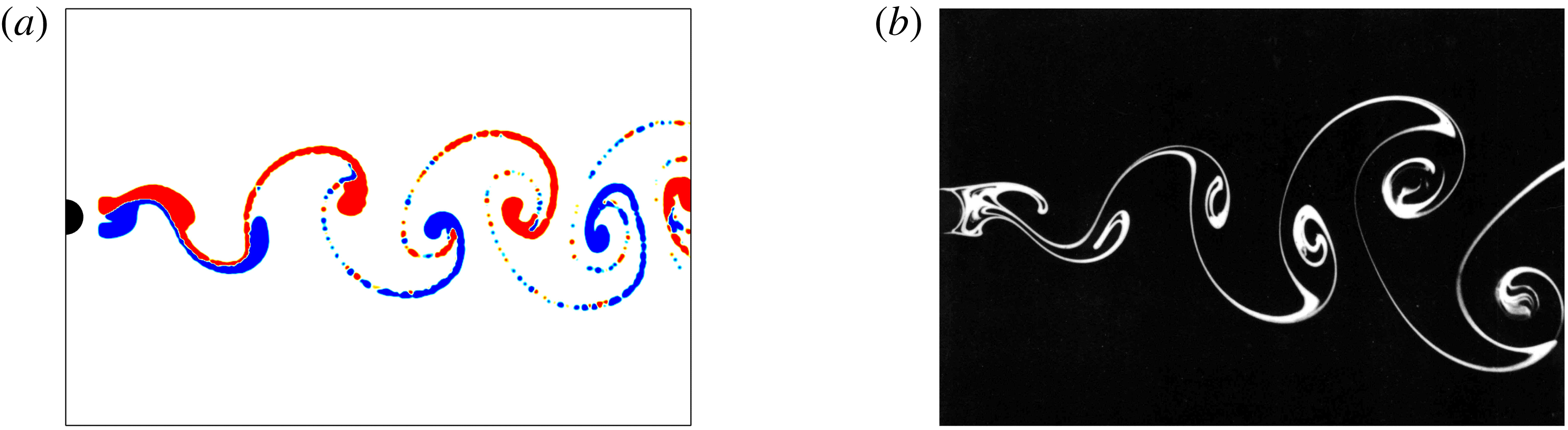
In the present study, the virtual tracers are first released from the initial locations continuously, then their trajectories are calculated from the PIV velocity data using the iterative algorithm of the ‘pseudo-tracing’ technique proposed by Jensen, Pedersen & Wood (Reference Jensen, Pedersen and Wood2003). This algorithm was used to calculate the material accelerations of virtual tracers by Liu & Katz (Reference Liu and Katz2006), and provides enough accuracy for the present calculation of trajectories. As the PIV velocity data are discrete, a cubic interpolation of the velocity data is used to obtain the local velocity of the tracers during the calculation of their trajectories. After a certain amount of time, the tracers in the flow would have converged onto the attracting LCS. At this point, the instantaneous coherent structures are revealed by merely checking the locations of the tracers in the flow at that time instant, however, here we take a further step to mimic the real dye. The tracers are treated as glittering particles that have a Gaussian distribution of intensity, and each instantaneous visualization image is an integration of the intensity of all the virtual tracers. This final step yields visualization results resembling those in real experiments, as shown in figure 2. Note that the initial releasing locations are close to the coherent structures to be visualized, however, it has been found that the final visualization result is not sensitive to the chosen locations as long as they are in the area influenced by the attracting LCS. The virtual dye visualization in figure 2(a) allows for the identification of upper and lower wake vortices, not only in terms of their transverse positions but also by their colours. This is extremely useful to reveal vortex interaction phenomenon, especially when the vortices make direct contact with each other, as will be shown later. It should be noted here that although the example in figure 2 is a laminar vortex street, the virtual dye visualization can be used to reveal attracting LCS in turbulent flow as well. This is because the tracers, when released from the locations under the influence of the attracting LCS, will eventually converge to the nearby separatrix that defines the attracting LCS, just as in real dye visualization of turbulent flows.
Visualizations of flow behind a circular cylinder. (a) Virtual dye visualization,
 $Re_{D}=158$
. The upper wake vortex is red in colour and the lower wake vortex is blue in colour. (b) Smoke visualization photographed by Sadatoshi Taneda, taken from Van Dyke (Reference Van Dyke1982),
 $Re_{D}=140$
.

4 Experimental results
The effects of gap height between the cylinder and the flat plate on the flow are shown in this section. Mean statistics are first presented in § 4.1, then the formation and downstream evolution of large spanwise vortices in the phase-averaged flow are discussed in § 4.2, and finally the interactions between the vortices are investigated in the instantaneous flow field in § 4.3.
4.1 Mean statistics
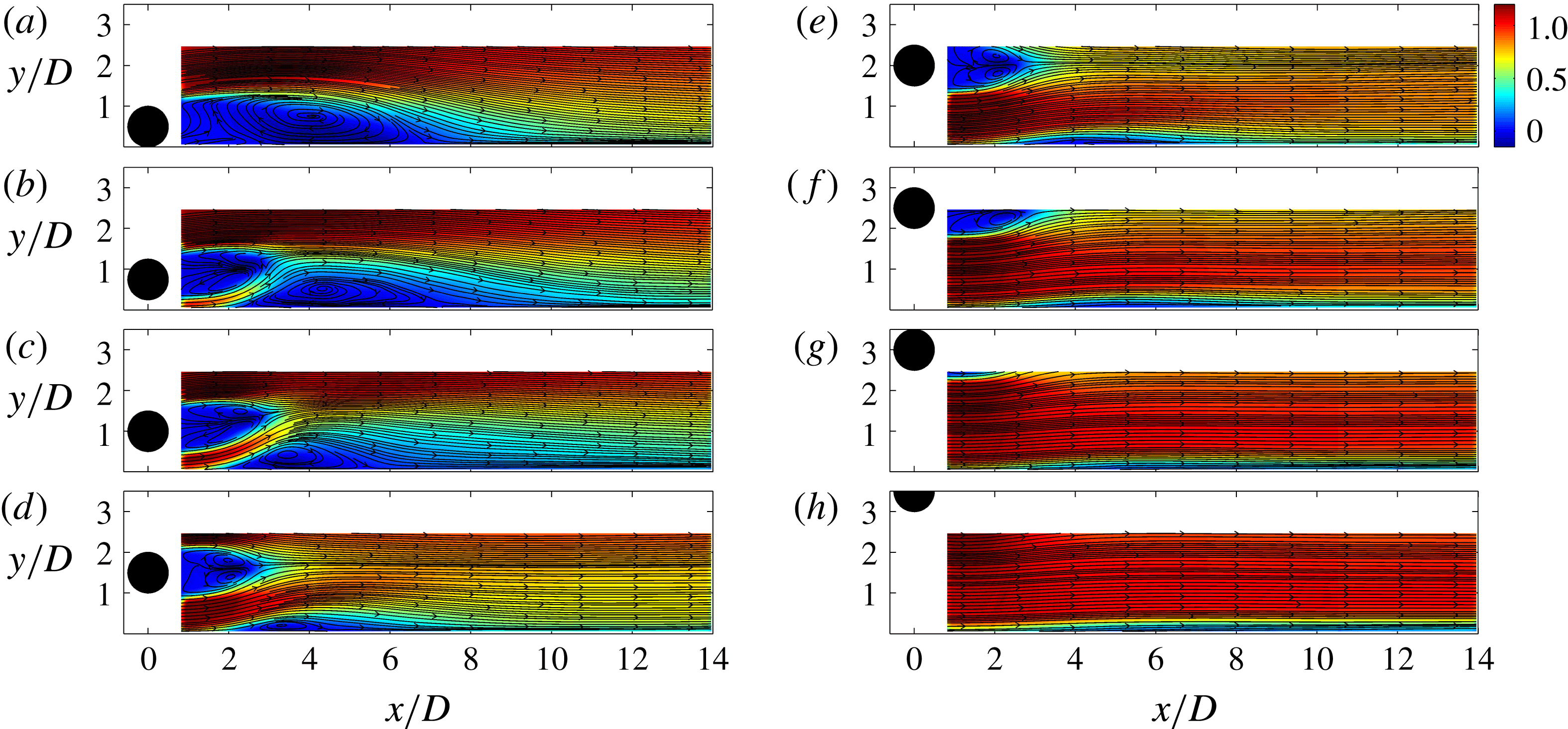
The mean streamwise velocity is shown in figure 3, which is represented in pseudo-colour with the mean streamlines superimposed on it. It is clear that the gap height has significant influence on the flow topology. In figure 3(a), the cylinder attaches to the wall (
 $G/D=0$
), the flow in this case resembles that behind a backward facing step. The flow past the upper side of the cylinder separates and forms a large separation bubble. The separation bubble reattaches to the wall at approximately
 $x/D=7$
. There is also a secondary bubble immediately behind the cylinder, which is only partly captured by the present measurement. As the cylinder leaves the wall, there is a gap flow under the cylinder (see figure 3
b,
 $G/D=0.25$
), the gap flow acts like a jet coming out of a slot due to the flow acceleration in the contracting tunnel formed by the lower front surface of the cylinder and the wall. The gap flow soon deflects away from the wall and penetrates through the separation bubble, leading to the formation of two large separation bubbles, an upstream one behind the cylinder and a downstream one on the wall. The deflection of the gap flow is related to the pairing between the boundary layer on the wall and the lower shear layer from the cylinder, which will be shown in the following figure.
Mean velocity in streamlines with the streamwise component in pseudo-colour. (a)
 $G/D=0$
, (b)
 $G/D=0.25$
, (c)
 $G/D=0.5$
, (d)
 $G/D=1.0$
, (e)
 $G/D=1.5$
, (f)
 $G/D=2.0$
, (g)
 $G/D=2.5$
, (h)
 $G/D=3.0$
.

In figure 3(c) at
 $G/D=0.5$
, the gap flow is much stronger, it deflects away from the wall and maintains considerable momentum when it makes contact with the upper shear layer of the cylinder, while for the case of
 $G/D=0$
.25 the gap flow is much weaker when it reaches the upper shear layer. The stronger gap flow brings more momentum into the recirculation region, consequently the separation bubble on the wall is reduced. It should be noted here that the contact between the gap flow and the upper shear layer implies a complex vortex interaction behaviour, which will be shown later. At
 $G/D=0.5$
, the separation bubble behind the cylinder contains two counter-rotating regions, indicating the probable onset of wake vortex shedding, although the bubble is asymmetric and tilts away from the wall. At
 $G/D=1.0$
(figure 3
d), the size of the separation bubble on the wall is significantly reduced and the asymmetry of the bubble behind the cylinder is still observable. When
 $G/D$
is increased to 1.5 (figure 3
e), the asymmetry of the separation bubble behind the cylinder is not obvious. Although no separation bubble is observed in the mean flow, by checking the instantaneous flow field (not shown here) it is found that a local separation occurs close to the wall in the form of a small patch of recirculation fluid. This local separation is periodical, which is associated with the formation of secondary vortices in the boundary layer. At
 $G/D=2.0$
, this local and periodical separation is still present very close to the wall in the instantaneous flow field. For
 $G/D=2.5$
and 3.0 (figure 3
g–h), no boundary layer separation can be observed in the mean flow or in the instantaneous flow field, and also secondary vortices are not observed. However, the growth of the boundary layer thickness downstream of the cylinder is obvious, indicating the transition still occurs under the wake perturbations.
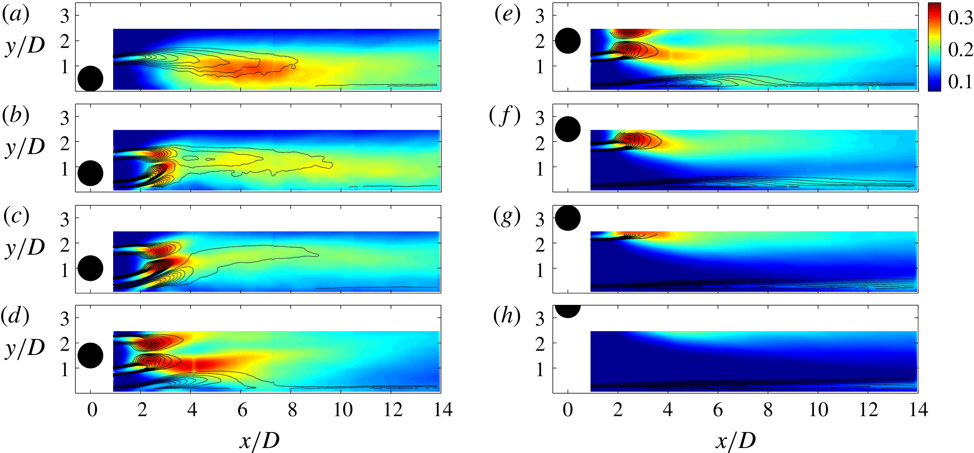
Figure 4 shows the root mean square of the streamwise velocity fluctuation
 $u_{rms}$
(in pseudo-colour) and the mean spanwise vorticity
 $\unicode[STIX]{x1D714}_{z}^{\ast }$
(in line contours). At
 $G/D=0$
in figure 4(a), the statistics is similar to that of a backward facing step. The shear layer separation from the upper side of the cylinder can be observed. At the present Reynolds number the shear layer can roll up into vortices, but the vortices are irregular and erratic, indicating that there is no dominant frequency of the flow.
 $u_{rms}$
growth initiates from the shear layer and reaches a considerable level in the region where the vortex rolling up occurs. For
 $G/D=0.25$
in figure 4(b) the flow is quite different. Three shear layers can be found downstream of the cylinder. Aside from the upper shear layer from the cylinder, two more shear layers are also present due to the gap flow, one is the lower shear layer from the cylinder and the other the separated boundary layer. Instead of cancelling each other, these two shear layers deflect away from the wall together, which is the so-called shear layer ‘pairing’ or ‘coupling’ described in previous studies (Price et al.
Reference Price, Sumner, Smith, Leong and Paidoussis2002; Sarkar & Sarkar Reference Sarkar and Sarkar2010). It should be kept in mind that the vorticity for upper shear layer and the separated boundary layer are negative (clockwise direction) while the vorticity for the lower shear layer is positive (counter-clockwise direction), so a single patch of vorticity after
 $x/D>4$
indicates that there may be some kind of merging process of the vorticity when these three regions of concentrated vorticity move close to each other. For
 $G/D=0.5$
in figure 4(c) the vorticity distribution is similar to that for
 $G/D=0.25$
, also similar is the active (high
 $u_{rms}$
value) wake region and the relatively calm near-wall region. However, the separated boundary layer seems to be much stronger than that for
 $G/D=0.25$
.
Mean vorticity
 $\unicode[STIX]{x1D714}_{z}^{\ast }$
in line contours with root mean square of the streamwise fluctuation
 $u_{rms}$
in pseudo-colour.
 $\unicode[STIX]{x1D714}_{z}^{\ast }$
is the normalized mean spanwise vorticity
 $\unicode[STIX]{x1D714}_{z}^{\ast }=\unicode[STIX]{x1D714}_{z}D/U_{\infty }$
.
 $u_{rms}$
is normalized by free-stream velocity
 $U_{\infty }$
. (a)
 $G/D=0$
, (b)
 $G/D=0.25$
, (c)
 $G/D=0.5$
, (d)
 $G/D=1.0$
, (e)
 $G/D=1.5$
, (f)
 $G/D=2.0$
, (g)
 $G/D=2.5$
, (h)
 $G/D=3.0$
.

For
 $G/D=1.0$
in figure 4(d), the deflections of the lower shear layer and the separated boundary layer are significantly reduced. The distribution of mean vorticity from the two sides of the cylinder is close to symmetry. The distribution of
 $u_{rms}$
, however, is quite asymmetric that the high value region (
 $u_{rms}/U_{\infty }>0.25$
) for the lower branch extends to approximately
 $x/D=7$
while that for the upper branch only reaches
 $x/D=4$
. As will be shown later, the larger high
 $u_{rms}$
region is closely related to the interaction between the lower wake vortex and the secondary vortex in the boundary layer. Further increase of
 $G/D$
makes the wake and boundary layer separately identifiable, as can be seen from the high
 $u_{rms}$
region near the wall in figure 4(e–h). Although the cylinder is already out of the camera’s field of view for high gap ratios, it is not difficult to deduce that as the cylinder moves away from the wall, the cylinder wake flow would be more and more like that of a stand-alone cylinder.
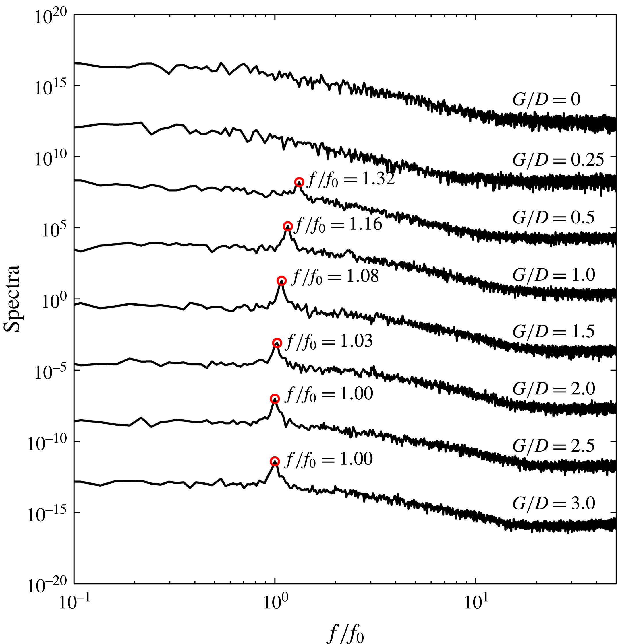
Streamwise velocity spectra for different gap ratios. The velocity traces were taken from the PIV data at a streamwise location of
 $x/D=3.0$
, and the wall-normal locations are
 $y/D=1.35$
, 1.0, 1.15, 1.18, 1.6, 2.08, 2.0 and 2.0 for
 $G/D=0$
, 0.25, 0.5, 1.0, 1.5, 2.0, 2.5 and 3.0, respectively. For
 $G/D\leqslant 2.0$
, the chosen wall-normal locations correspond to local maxima of
 $u_{rms}$
, while for
 $G/D=2.5$
and 3.0, a maximum of
 $u_{rms}$
in the wake region is not available and
 $y/D=2.0$
is used instead. The frequency is normalized by
 $f_{0}$
, where
 $f_{0}$
is the wake vortex shedding frequency at
 $G/D=3.0$
.

The streamwise velocity spectra for different gap ratios are shown in figure 5. The velocity traces are taken at the streamwise location of
 $x/D=3.0$
, and the wall-normal locations are chosen to be at the local maxima of
 $u_{rms}$
which vary with
 $G/D$
. For
 $G/D\geqslant 0.5$
there is a dominant peak on the spectrum, which indicates the frequency of wake vortex shedding from the cylinder. For a fixed
 $G/D$
, this characteristic frequency does not change when the probe is placed in a number of different locations in the flow, meaning that the characteristic frequency of the vortex dynamics remained unchanged. However, figure 5 shows that with the decrease of
 $G/D$
, the characteristic frequency increases. For
 $G/D=0$
and 0.25, where the lower shear layer from the cylinder is inhibited or completely suppressed, no distinguished peaks can be observed on the spectra.
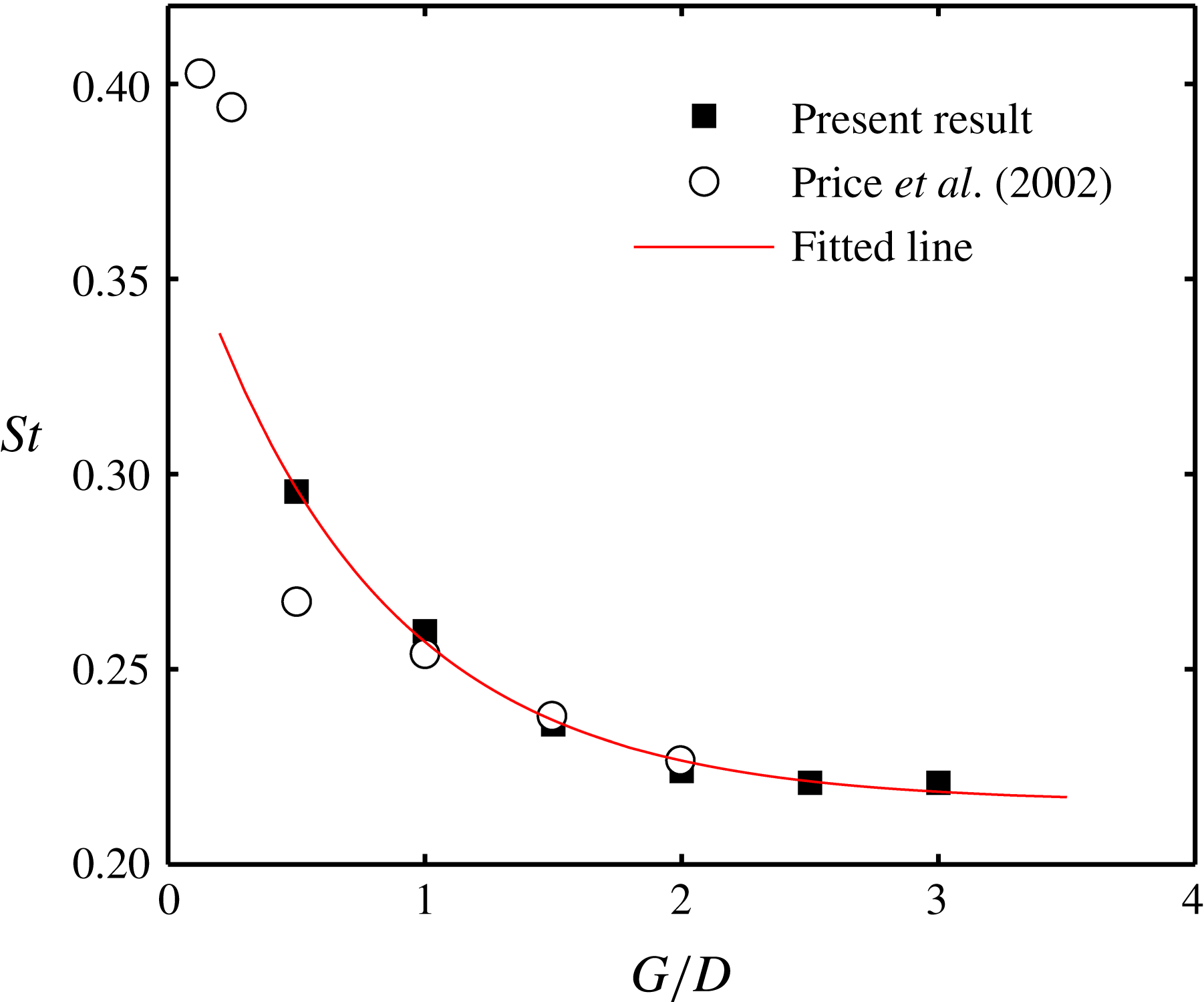
The dominant frequencies determined in figure 5 is plotted against the gap ratio in figure 6. As shown in figure 6 the Strouhal number
 $St$
(
 $St=fD/U_{\infty }$
) increases with decreasing gap ratio. The variation of
 $St$
is fitted very well by an exponential curve:
 $St=0.16\exp (-1.34G/D)+0.21$
, where 0.21 is the
 $St$
for a stand-alone circular cylinder. Price et al. (Reference Price, Sumner, Smith, Leong and Paidoussis2002) has already reported the change of
 $St$
as the cylinder approaches the wall at low Reynolds number (
 $Re_{D}<2600$
) and that
 $St$
was insensitive to
 $G/D$
at higher Reynolds number. The present
 $Re_{D}$
is in their low Reynolds number range and the variation of
 $St$
is quite considerable, from 0.22 at
 $G/D=3.0$
to 0.29 at
 $G/D=0.5$
, with nearly a 32 % increase. The
 $St$
in the present study compares well with that of Price et al. (Reference Price, Sumner, Smith, Leong and Paidoussis2002) for
 $G/D\geqslant 1.0$
. At
 $G/D=0.5$
, however, the difference is significant. Moreover, below
 $G/D=0.25$
, no dominant frequency in the spectra can be found in present study, while Price et al. (Reference Price, Sumner, Smith, Leong and Paidoussis2002) claimed that there did not seem to be a minimum value of
 $G/D$
below which periodicities were not detected in the wake. The
 $St$
in the study of Price et al. (Reference Price, Sumner, Smith, Leong and Paidoussis2002) can be as high as approximately 0.4 at
 $G/D=0.125$
. Price et al. (Reference Price, Sumner, Smith, Leong and Paidoussis2002) explained that it was more properly associated with periodicities in the outer shear layer from the cylinder instead of classical vortex shedding. In the present study, however, such periodicities in the outer shear layer cannot be found. This difference for low gap ratios between the present study and that of Price et al. (Reference Price, Sumner, Smith, Leong and Paidoussis2002) may be attributed to the different boundary layer thicknesses at the location of the cylinder (
 $\unicode[STIX]{x1D6FF}/D=0.53$
in the present study and
 $\unicode[STIX]{x1D6FF}/D=0.45$
in their study). Price et al. (Reference Price, Sumner, Smith, Leong and Paidoussis2002) did not give an explanation for the change of
 $St$
at low Reynolds number, which can be expected to be strongly related to the vortex dynamics and will be explored in the present study.
Vortex shedding frequency at different gap ratios.
 $St=fD/U_{\infty }$
. The fitted line is expressed as
 $St=0.16\exp (-1.34G/D)+0.21$
and only the data in the present study are taken into account.

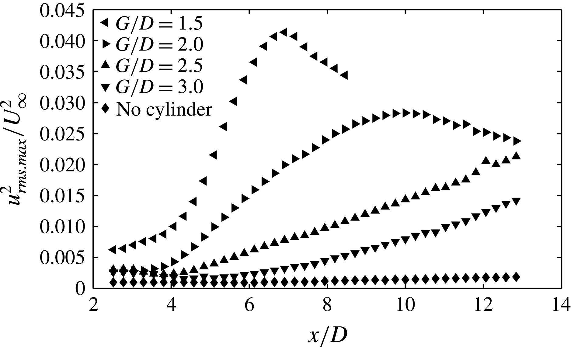
Figure 7 shows the disturbance growth inside the boundary layer for
 $G/D\geqslant 1.5$
. As shown in figure 4, for these gap ratios the boundary layer can be identified separately. For
 $G/D<1.5$
, due to the separation of the boundary layer from the wall, the amplification of the disturbance occurs in the separated shear layer, which extends into the wake and results in turbulence generation mainly in the wake region (see figure 4). When the cylinder is absent, the disturbance in the laminar boundary layer varies little and is at about the level of the background noise. With the presence of the cylinder, disturbance growth will initiate downstream of the cylinder due to the transition triggered by the wake perturbations. The closer the cylinder is to the wall, the faster the disturbance growth will be. For the cases of
 $G/D=1.5$
and 2.0, the transition is featured by the evolution of secondary vortices in the boundary layer, a transition route that has been investigated by previous researchers, such as Pan et al. (Reference Pan, Wang, Zhang and Feng2008), Mandal & Dey (Reference Mandal and Dey2011) and He et al. (Reference He, Wang and Pan2013, Reference He, Pan, Feng, Gao and Wang2016) (which has been described in the introduction). He et al. (Reference He, Wang and Pan2013) pointed out that the fast disturbance growth in the boundary layer is related to the three-dimensional destabilization of the initially nearly two-dimensional spanwise secondary vortices. The disturbance reaches a peak at around
 $x/D=7$
and
 $x/D=10$
for
 $G/D=1.5$
and
 $G/D=2.0$
, respectively. Afterwards the disturbance begins to decay when the flow becomes highly nonlinear. The lack of data points for
 $G/D=1.5$
downstream of
 $x/D=8.5$
is due to the merging of the boundary layer with the wake.
Disturbance growth in the boundary layer;
 $u_{rms.max}$
is the maximum of
 $u_{rms}$
in the boundary layer.

For
 $G/D=2.5$
and 3.0, the disturbance growth is slower than the previous two cases, but still much faster than the case of smooth boundary layer without the presence of the cylinder. As we have mentioned earlier, there are no secondary vortices in the boundary layer and the transverse expansion of the turbulence in the wake has not reached the boundary layer yet in the measured field of view for these two cases, so the transition of the boundary layer may well be attributed to the influence of an adverse pressure gradient. In the experiment of Bearman & Zdravkovich (Reference Bearman and Zdravkovich1978), they found that the presence of the circular cylinder in proximity to the wall would introduce a minimum of the pressure coefficient on the wall downstream of the cylinder. This means an adverse pressure gradient (APG) further downstream, and the closer the cylinder is to the wall, the higher the APG will be. Therefore, in the present study, when the cylinder is close enough to the wall (
 $G/D<1.5$
), the large APG leads to a constant separation of the boundary layer. When the gap ratio is moderate (
 $G/D=1.5$
and
 $G/D=2.0$
), the moderate APG (which is fluctuating with the wake) can only periodically induce a local separation of the boundary layer, leading to the formation of secondary vortices which convect downstream close to the wall. When the gap ratio is increased to
 $G/D=2.5$
and 3.0, the APG may be too weak to induce any separation, however, the APG is known to make the boundary layer more unstable and facilitates transition, therefore boundary layer disturbance growth is observed downstream of the cylinder.
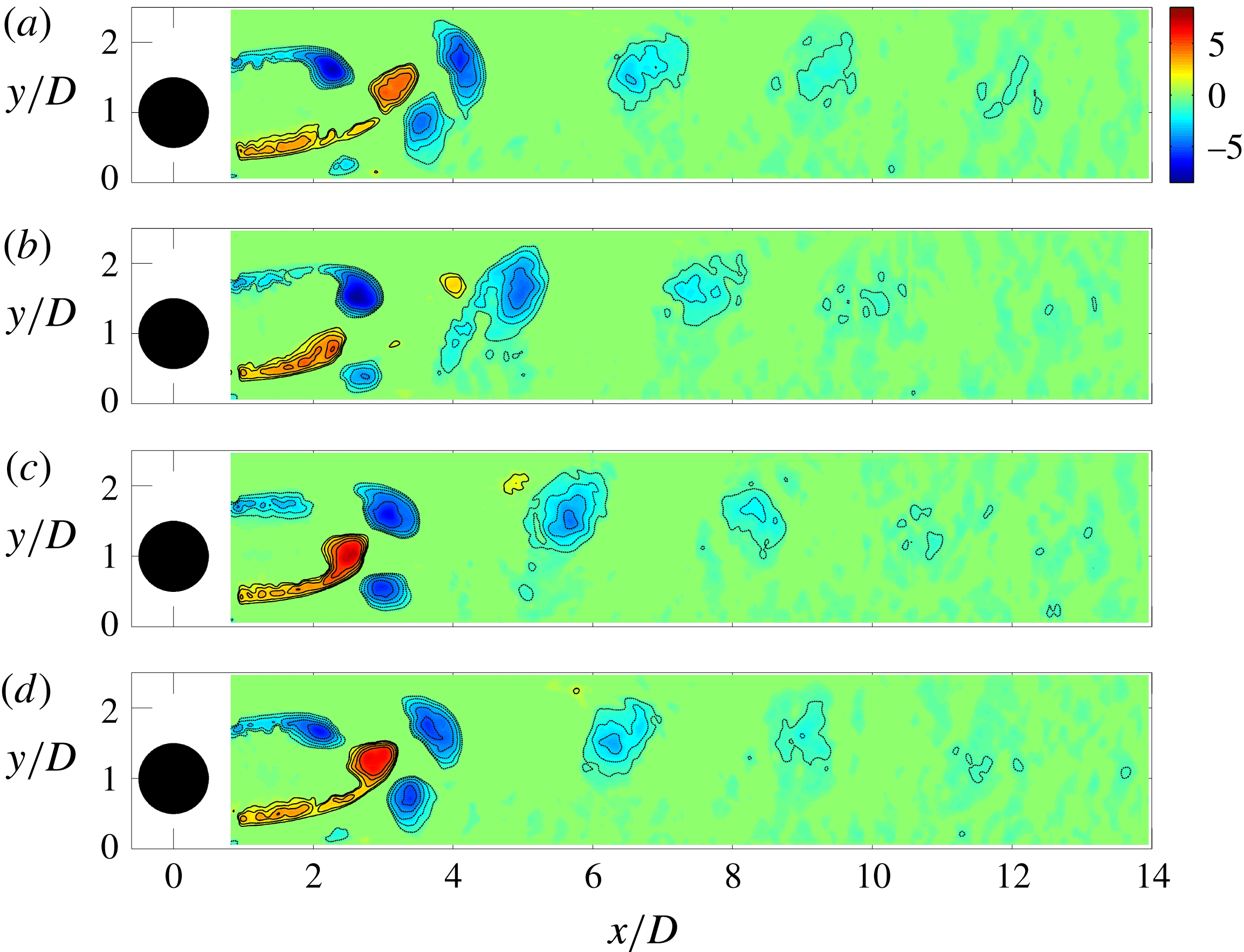
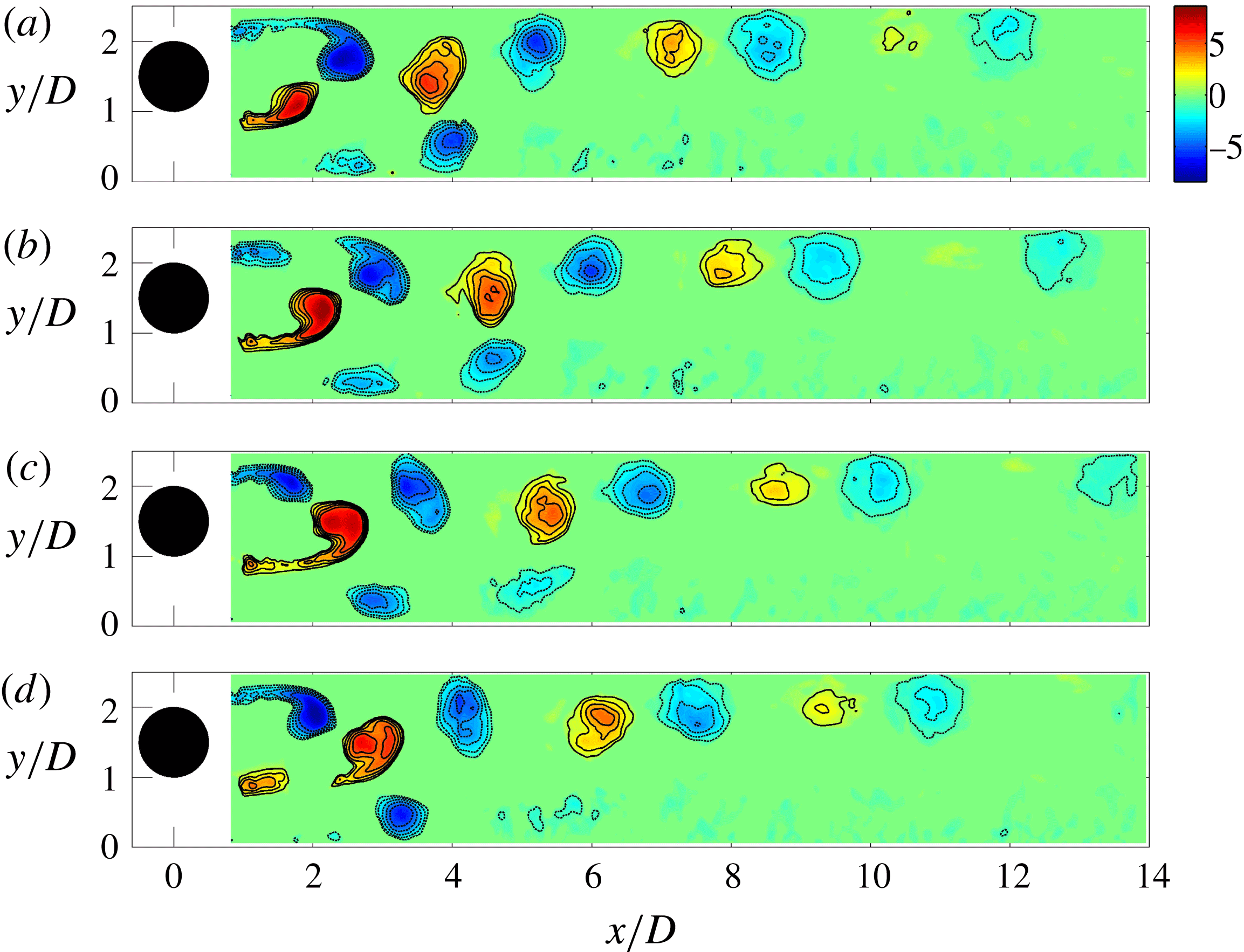
Phase-averaged
 $\unicode[STIX]{x1D706}_{ci}$
field,
 $G/D=0.5$
. Positive (counter-clockwise rotating) vortices are in red colour and solid contour lines, while negative (clockwise rotating) vortices are in blue colour and dashed contour lines, the lowest contour level is
 $\unicode[STIX]{x1D706}_{ci}=1$
and increment between contour lines is 1. (a)
 $\unicode[STIX]{x1D6F7}=0^{\circ }$
, (b)
 $\unicode[STIX]{x1D6F7}=90^{\circ }$
, (c)
 $\unicode[STIX]{x1D6F7}=180^{\circ }$
, (d)
 $\unicode[STIX]{x1D6F7}=270^{\circ }$
. See supplementary movie 1 available online at https://doi.org/10.1017/jfm.2016.812.

4.2 Phase-averaged vortical structures
This section presents the spanwise vortical structures in phase-averaged flow field for three cases of
 $G/D=0.5$
, 1.0 and 2.0, which are representative of vortex dynamics in cylinder wake/boundary layer interactions. For
 $G/D>2.0$
, no vortical structures (boundary layer separation) is observed in the near-wall region downstream of the cylinder and the wake vortices of the cylinder are just like that of a stand-alone cylinder. For
 $G/D<0.5$
, no clear periodicity can be determined, therefore phase averaging is not possible. In performing the phase averaging, the frames at a certain phase angle are determined with a cross-correlation between all the velocity frames with the base frame and then selecting the ones corresponding to the correlation peaks. These selected frames are averaged to yield the flow field at that phase angle. This step is repeated until averaged flow fields are extracted at all the needed phase angles. The vortices are identified from the phase-averaged flow field by the
 $\unicode[STIX]{x1D706}_{ci}$
method proposed by Zhou et al. (Reference Zhou, Adrian, Balachandar and Kendall1999).
 $\unicode[STIX]{x1D706}_{ci}$
is the imaginary part of the complex eigenvalue of the velocity gradient tensor. In the present study,
 $\unicode[STIX]{x1D706}_{ci}$
is computed from the two-dimensional truncated velocity gradient tensor due to the limitation of two-dimensional PIV measurement. The sign of the local vorticity is assigned to the
 $\unicode[STIX]{x1D706}_{ci}$
to indicate the rotation sense.
Phase-averaged
 $\unicode[STIX]{x1D706}_{ci}$
field,
 $G/D=1.0$
. (a)
 $\unicode[STIX]{x1D6F7}=0^{\circ }$
, (b)
 $\unicode[STIX]{x1D6F7}=90^{\circ }$
, (c)
 $\unicode[STIX]{x1D6F7}=180^{\circ }$
, (d)
 $\unicode[STIX]{x1D6F7}=270^{\circ }$
. See supplementary movie 2.

In figure 8 at
 $G/D=0.5$
, phase-averaged results show that the alternative wake vortex shedding has already been restored. However, the shedding is asymmetric about the centreline of the cylinder, the upper wake vortex moves nearly parallel with the wall while the lower wake vortex moves away from the wall and even surpasses the height of the upper one. This result is what Sarkar & Sarkar (Reference Sarkar and Sarkar2010) described as cross-over of the vortex trajectories and inversion of the vortex positions, with the wake vortex from the lower side of the cylinder being above the one from the upper side. During this cross-over, the lower wake vortex shrinks very fast and soon loses its trace. Aside from the two wake vortices, there is another vortex below the lower one. This vortex is formed by the rolling up of the separated boundary layer that pairs with the lower shear layer. It rotates in the opposite direction to the lower wake vortex and has the same shedding frequency as the latter. We denote it the secondary vortex as it can be regarded as being induced by the passing wake vortices, as a result of vortex-induced instability of wall-bounded shear layers (Sengupta, De & Sarkar Reference Sengupta, De and Sarkar2003; Dipankar & Sengupta Reference Dipankar and Sengupta2005). The separated boundary layer becomes turbulent as it gradually merges into the wake (see figure 4
c), and the flow finally reattaches onto the wall, forming a separation bubble (see figure 3
c). It should be emphasized that the secondary vortex is an instantaneous vortical structure while the separation bubble is based on the mean streamlines. The separation bubble, although having closed or spiral mean streamlines, does not represent the secondary vortex which is much smaller in size and convects with the flow. In figure 8 the secondary vortex moves away from the wall together with the lower wake vortex. When it moves close to the upper wake vortex it seems to merge with the latter and lose its identity very quickly. The above results suggest that at
 $G/D=0.5$
, these three vortices come very close to each other and have direct interactions among them. The upper wake vortex and the secondary vortex have the same rotation sense and seem to merge together while the lower wake vortex may be canceled because it has the opposite sign and is relatively weaker than the sum of the other two vortices. Consequently, only negative vortices (clockwise rotating) are observed in the downstream wake.
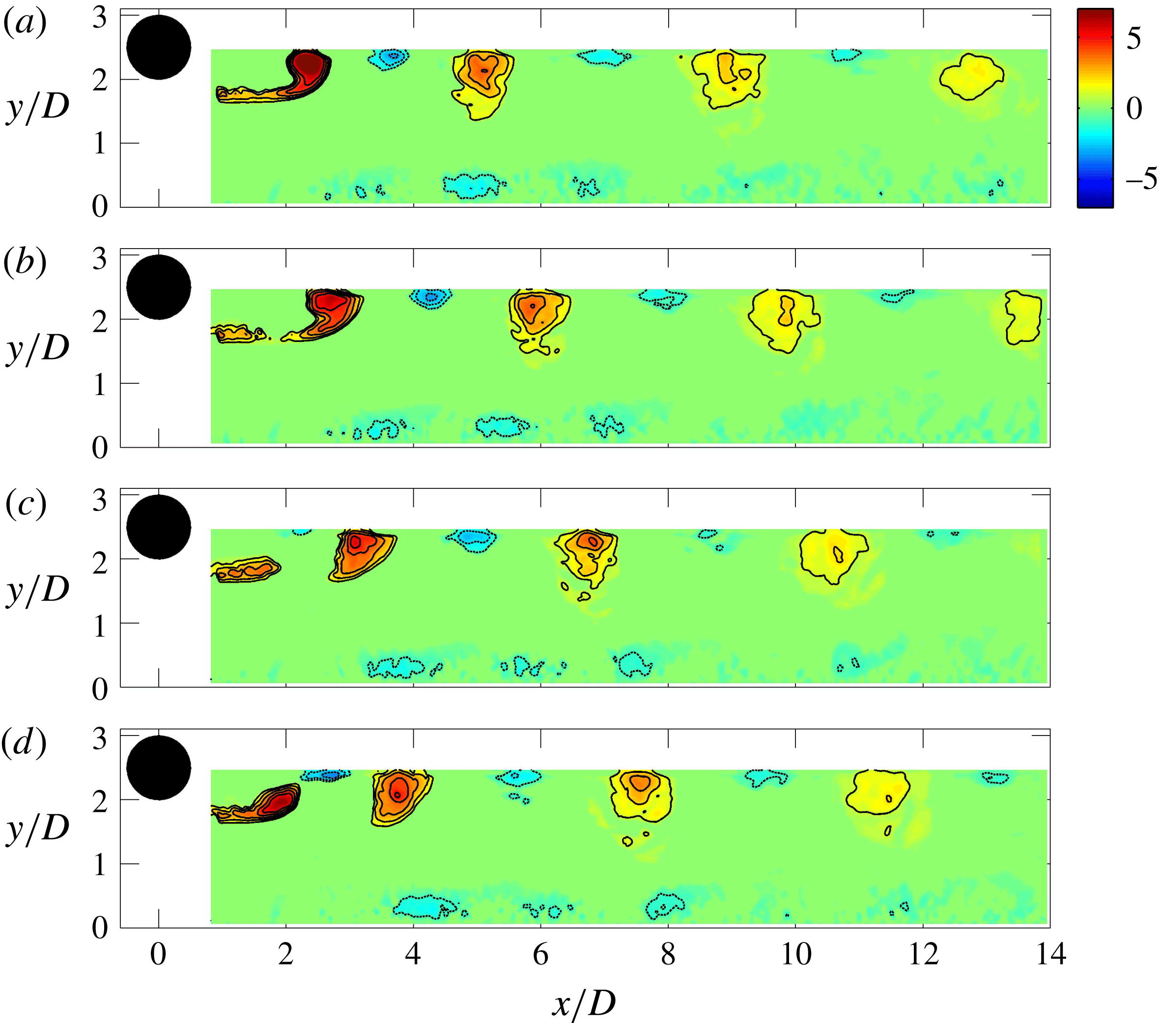
Phase-averaged
 $\unicode[STIX]{x1D706}_{ci}$
field,
 $G/D=2.0$
. (a)
 $\unicode[STIX]{x1D6F7}=0^{\circ }$
, (b)
 $\unicode[STIX]{x1D6F7}=90^{\circ }$
, (c)
 $\unicode[STIX]{x1D6F7}=180^{\circ }$
, (d)
 $\unicode[STIX]{x1D6F7}=270^{\circ }$
. See supplementary movie 3.

In figure 9 at
 $G/D=1.0$
, the three vortices in the previous case are still present. The lower wake vortex still moves away from the wall, but it only gets elevated to the same height as the upper wake vortex. At this gap ratio, the lower wake vortex convects for a longer streamwise distance than that at
 $G/D=0.25$
, but still decays faster than the upper wake vortex. The lift-up of the secondary vortex is also reduced and it can no longer interact with the upper wake vortex. Alternatively, the interaction at this gap ratio is mainly between the secondary vortex and the lower wake vortex, which cannot be seen from this phase-averaged result. One previous study of He et al. (Reference He, Wang and Pan2013) at
 $G/D=1.0$
has revealed through visualization that after the secondary vortex is formed in the near-wall region and gets lifted up, it directly interacts with the lower wake vortex after
 $x/D=4$
. Because the secondary vortex has the opposite rotation sense to the lower wake vortex and is weaker than the latter, it ends up either being rolled up into the wake or being pushed down to the wall, depending on its relative position with the lower wake vortex. This interaction results in the fast breakdown of the secondary vortex which can be observed in the near-wall region of figure 9. The interaction also results in an increased turbulence level in the related region and causes the asymmetry of the turbulent statistics (
 $u_{rms}$
in figure 4
d). Although the lower wake vortex is less affected by this interaction, the increased turbulence level facilitates its breakdown into small vortices and therefore it appears to decay faster than the upper wake vortex.
In figure 10 at
 $G/D=2.0$
, the secondary vortex and the lower wake vortex are shown, as well as part of the upper wake vortex. It can be seen that the lower wake vortex moves nearly parallel with the wall and so does the secondary vortex. In this case, the distance between the secondary vortex and the lower wake vortex prevents any direct interactions from happening. However, the wake provides perturbations that can promote the destabilization of the secondary vortices. The evolution of the secondary vortices has been investigated by recent studies of Pan et al. (Reference Pan, Wang, Zhang and Feng2008) and He et al. (Reference He, Wang and Pan2013, Reference He, Pan, Feng, Gao and Wang2016). It has been revealed that the spanwise secondary vortex develops three-dimensional instability under the perturbation of the wake and deforms into
 $\unicode[STIX]{x1D6EC}$
vortices, which further evolve into hairpin vortices. The hairpin vortices can generate new hairpin vortices in a hierarchy, leading to the formation of hairpin packets in the final turbulent boundary layer.
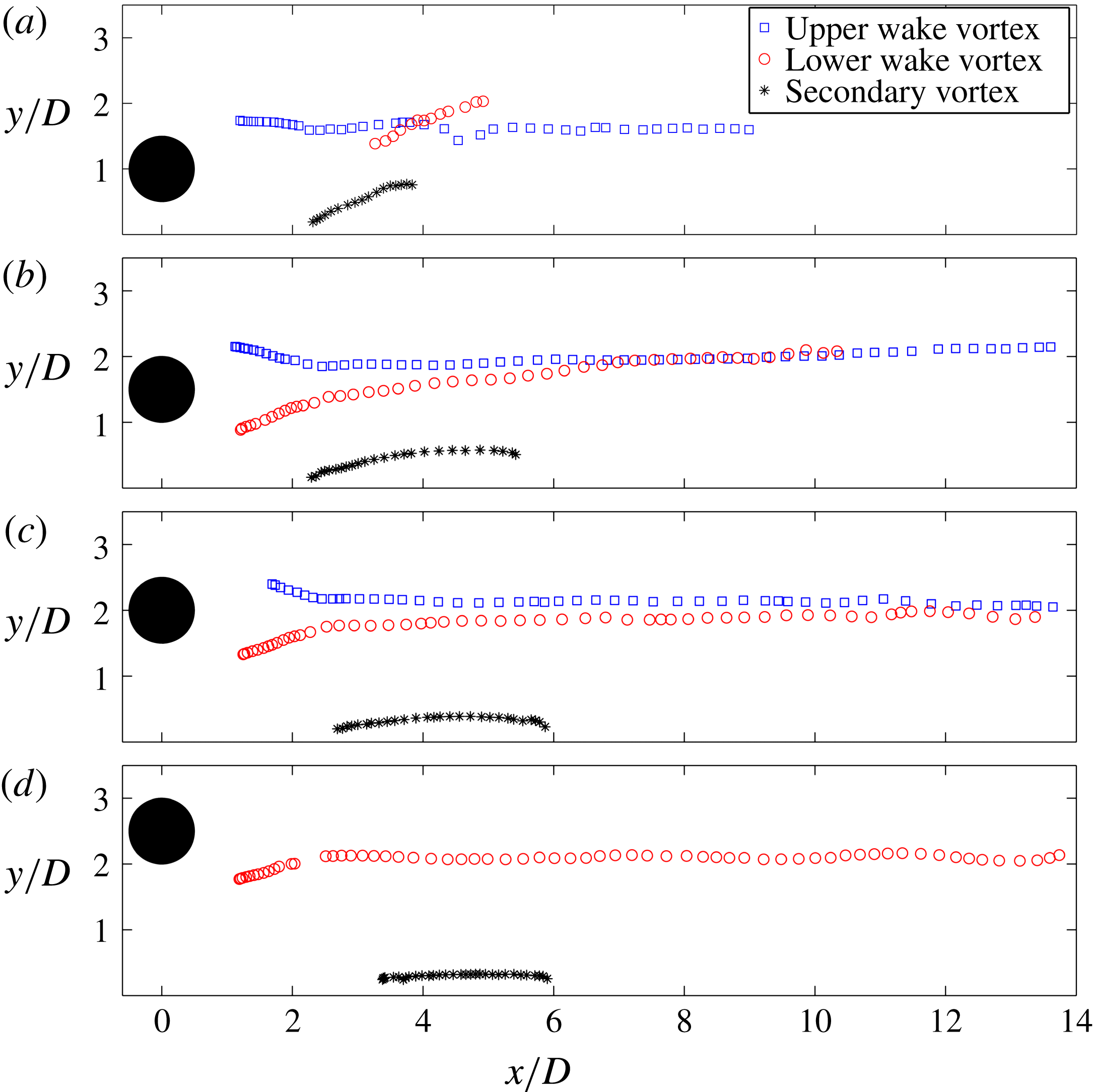
Trajectories of vortices. (a)
 $G/D=0.5$
, (b)
 $G/D=1.0$
, (c)
 $G/D=1.5$
, (d)
 $G/D=2.0$
.

The trajectories of the large spanwise vortices in the phase-averaged flow field are shown in figure 11 for
 $G/D=0.5$
, 1.0, 1.5 and 2.0. The vortex centres are identified as the weighted centroid of the
 $\unicode[STIX]{x1D706}_{ci}$
concentration region with threshold of
 $\unicode[STIX]{x1D706}_{ci}^{\text{T}}=1.0$
. As discussed in the previous section, the gap ratio has a huge impact on the trajectories of lower wake vortex and the secondary vortex, while the trajectory of the upper wake vortex is little affected and nearly parallel to the wall for all gap ratios tested. At
 $G/D=0.5$
, the lift-up of the secondary vortex and the lower wake vortex is quite obvious and the trajectories of the upper and lower wake vortices clearly cross each other, resulting in the inversion of their positions, as mentioned above. The lower wake vortex and the secondary vortex lose their traces very fast. This is due to their interactions with the upper wake vortices which will be shown later in detail by the instantaneous vortical structures. At
 $G/D=1.0$
, the angles of the secondary vortex and the lower wake vortex convecting away from the wall are reduced. The lower wake vortex can reach the height of that of the upper wake vortex but there is no cross-over of the trajectories. The lower wake vortex in this case persists longer but still ‘diminishes’ faster than the upper wake vortex. With the increased gap ratio the deflection angles further decrease (see figure 11
c,d). By
 $G/D=2.0$
, trajectories of both the secondary vortex and the lower wake vortex are nearly parallel to the wall, the trajectory of the upper wake vortex cannot be given because it is only partly captured in the present field of view (see figure 10).
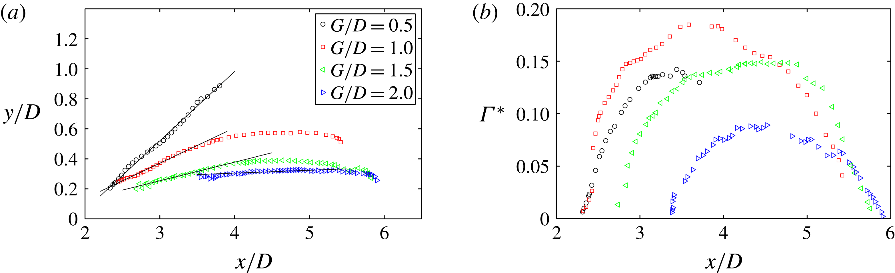
A direct comparison of secondary vortex trajectories at different gap ratios is presented in figure 12(a). The initial lift-up of the secondary vortex trajectories seems to be a linear increase and is fitted with straight lines to yield the deflection angles. The deflection angles for the cases of
 $G/D=0.5$
, 1.0, 1.5, 2.0 are
 $25^{\circ }$
,
 $11^{\circ }$
,
 $6^{\circ }$
and
 $1^{\circ }$
, respectively, showing the large variation in convection direction of the secondary vortex. Figure 12(b) gives the normalized circulation
 $\unicode[STIX]{x1D6E4}^{\ast }$
of the secondary vortices for the above four cases. Downstream of the cylinder, the secondary vortex forms in terms of accumulation of vorticity from the boundary layer, so a continual growth of the
 $\unicode[STIX]{x1D6E4}^{\ast }$
can be observed. The formation process can be deemed complete when
 $\unicode[STIX]{x1D6E4}^{\ast }$
reaches its peak. The decrease of
 $\unicode[STIX]{x1D6E4}^{\ast }$
afterwards is related to the further development of the secondary vortices, including three-dimensional deformation or even disintegration. It can be observed from figure 12(b) that as the cylinder approaches the wall (
 $G/D=2.0$
, 1.5 and 1.0) but stays out of the boundary layer (
 $\unicode[STIX]{x1D6FF}/D=0.53$
), the growth of
 $\unicode[STIX]{x1D6E4}^{\ast }$
initiates earlier and the peak value is larger, which is the result of stronger interaction between the cylinder wake and the boundary layer. The maximum
 $\unicode[STIX]{x1D6E4}^{\ast }$
can be found for
 $G/D=1.0$
. At
 $G/D=0.5$
, however, the secondary vortex is weaker than the case of
 $G/D=1.0$
, this is because the cylinder is already positioned in the outer part of the boundary layer and the lower shear layer from the cylinder is suppressed, therefore the induced secondary vortex is weaker. It should be noted that at
 $G/D=0.5$
the secondary vortex loses its trace very early near
 $x/D=4$
without a continual decrease as in the higher gap ratio cases, which is due to its interaction with the upper wake vortex (shown in the following).
(a) Trajectories and (b) circulation of secondary vortices.
 $\unicode[STIX]{x1D6E4}^{\ast }$
in (b) is the normalized circulation,
 $\unicode[STIX]{x1D6E4}^{\ast }=\unicode[STIX]{x1D6E4}/(\unicode[STIX]{x03C0}DU_{\infty })$
.

4.3 Instantaneous vortical structures
The formation and convection of vortices shown above are in phase-averaged flow, where the turbulent fluctuation and small-scale structures are smoothed out to allow attention to be paid to large periodical structures. The results also show indications of vortex interaction when they move close enough to each other for low gap ratios such as
 $G/D=0.5$
. The interaction often leads to the final disintegration or breakdown of vortices, which can only be shown in detail in the instantaneous flow field with a proper visualization method. At the Reynolds number in the present study, the wake is turbulent, therefore the vorticity plot of a vortex in the instantaneous flow is irregular in shape and may emerge in pieces before interaction (see Sarkar & Sarkar Reference Sarkar and Sarkar2010). Moreover, it is almost impossible to distinguish the vorticity of two same-signed vortices as soon as they make contact. Therefore, the vorticity plot is perhaps not an appropriate way to investigate vortex interactions in the present study and an alternative method of virtual dye visualization is applied instead.
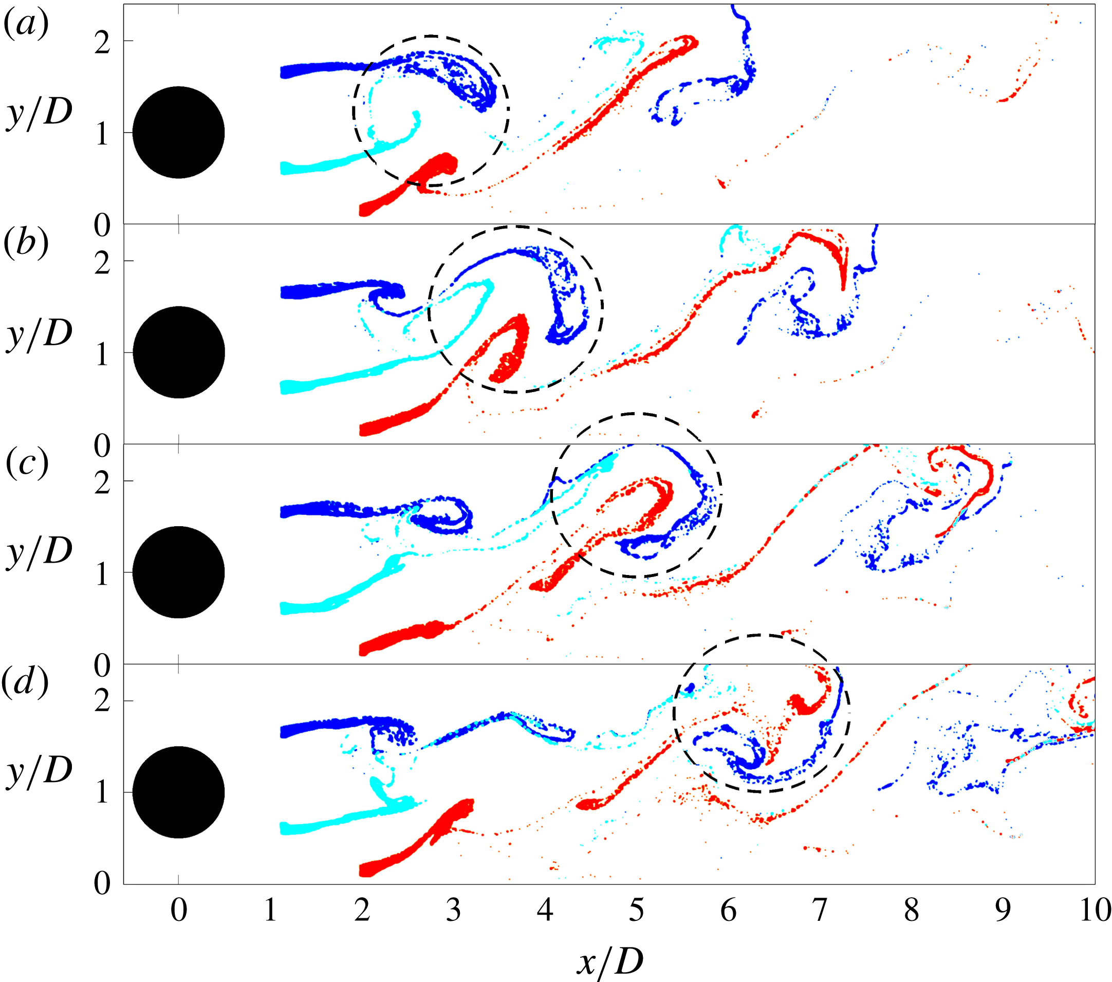
In the present study, we use virtual dye visualization with a particular purpose: to reveal the complex vortex interactions. The virtual dye is released in the upper shear layer, lower shear layer and the boundary layer at the same time, the corresponding upper wake vortex, the lower wake vortex and the secondary vortex are then visualized, respectively.
Instantaneous vortical structures,
 $G/D=0.5$
. (a)
 $t$
, (b)
 $t+\unicode[STIX]{x0394}t$
, (c)
 $t+2\unicode[STIX]{x0394}t$
, (d)
 $t+3\unicode[STIX]{x0394}t$
,
 $\unicode[STIX]{x0394}t/T_{0.5}=0.3$
, where
 $T_{0.5}$
is the vortex shedding period for
 $G/D=0.5$
. The upper wake vortex, the lower wake vortex and the secondary vortex are tagged in blue, cyan and red colours, respectively. See supplementary movie 4.

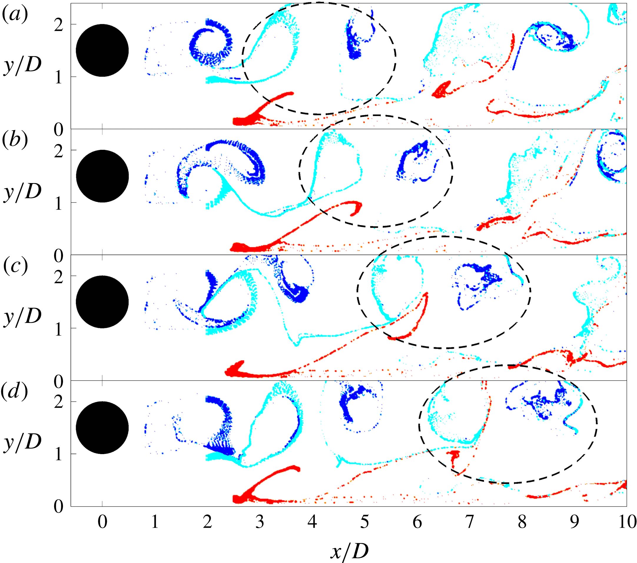
Instantaneous vortical structures,
 $G/D=1.0$
. (a)
 $t$
, (b)
 $t+\unicode[STIX]{x0394}t$
, (c)
 $t+2\unicode[STIX]{x0394}t$
, (d)
 $t+3\unicode[STIX]{x0394}t$
,
 $\unicode[STIX]{x0394}t/T_{1.0}=0.26$
, where
 $T_{1.0}$
is the vortex shedding period for
 $G/D=1.0$
. The upper wake vortex, the lower wake vortex and the secondary vortex are tagged in blue, cyan and red colours, respectively. See supplementary movie 5.

At
 $G/D=0.5$
in figure 13, the formation of upper wake vortex, the lower wake vortex and the secondary vortex are clearly revealed. Our focus here is on the subsequent interaction among them. As mentioned earlier, vortex interaction occurs when the lower wake vortex and the secondary vortex move up towards the upper wake vortex (as shown by the circled area). One should remember that the upper wake vortex and the secondary vortex have the same sign and rotate in the clockwise direction while the lower wake vortex has the opposite sign. It can be observed in figure 13 that the three vortices are all stretched to some extent, but the lower wake vortex is stretched the most. Besides, the lower wake vortex and the secondary vortex are gradually encompassed by the upper wake vortex and its tail, which is usually a thin shear layer following a shed wake vortex. During the interaction process, the lower wake vortex is under severe stretching while the upper wake vortex and the secondary vortex can maintain their vortical shapes and rotate about each other, typically seen in the merging of two co-rotating vortices in a mixing layer which is called ‘vortex pairing’ (Winant & Browand Reference Winant and Browand1974). In figure 13(d) the lower wake vortex has been stretched almost into a thin layer and can be regarded as having already broken down, a process similar to the ‘vortex tearing’ in a mixing layer (Moore & Saifman Reference Moore and Saifman1975; Saffman & Baker Reference Saffman and Baker1979), where the vorticity of one vortex is entrained and absorbed into the other vortices. In figure 13(d) the upper wake vortex and the secondary vortex nearly switch their relative positions as compared with figure 13(a), they go through further deformation and seem to penetrate into each other, a stage which can be more clearly revealed by the late-stage vortex interaction from the previous shedding period in the downstream region of
 $x/D=7{-}8$
in figure 13(b,c). This indicates the merging of these two same-signed vortices. So the result of the vortex interaction in this case is the merging of upper wake vortex and the secondary vortex, and the breakdown of the lower wake vortex. This explains why only clockwise rotating vortices are detected downstream. The terms ‘vortex tearing’ and ‘vortex pairing’ are two mechanisms proposed to explain the disappearance or disintegration of vortices in mixing layers and obviously they both have particular implications in the present complex flow scenario.
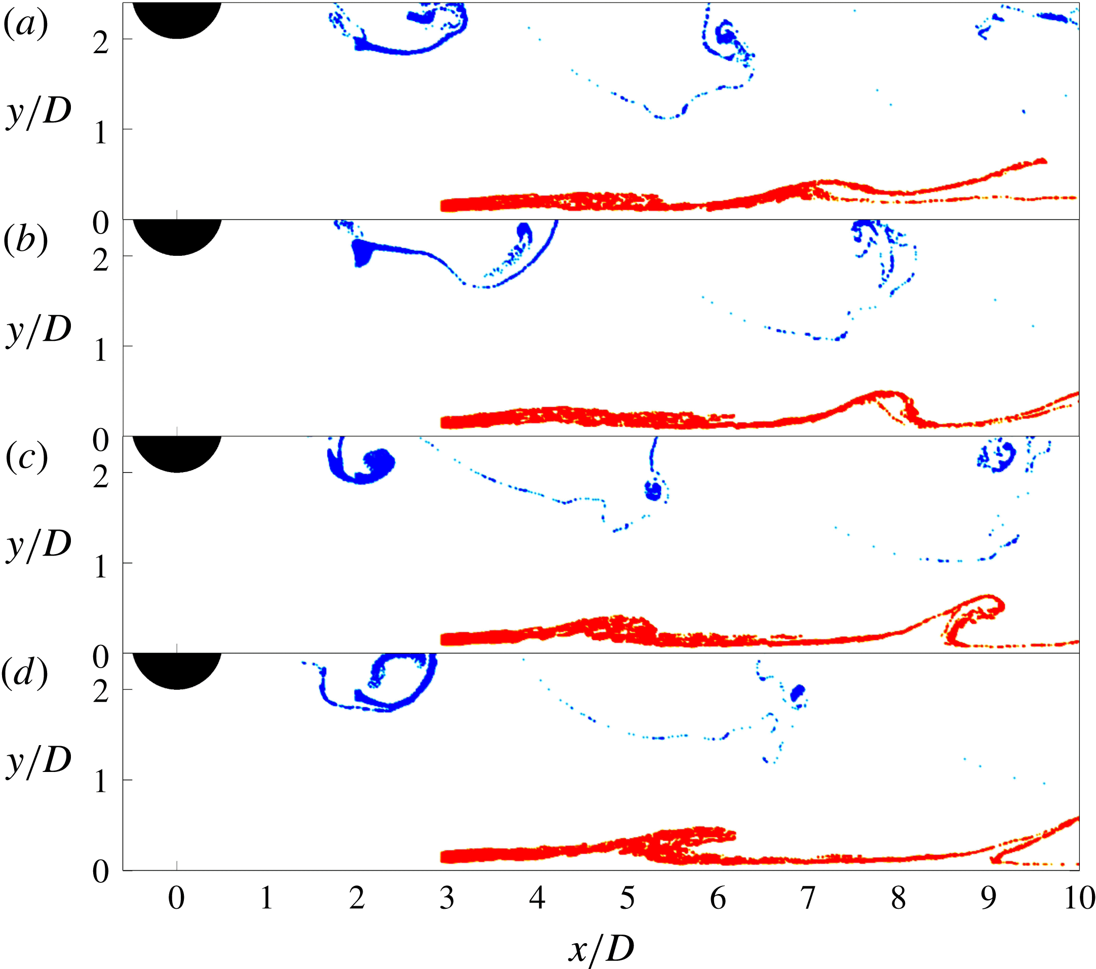
Instantaneous vortical structures,
 $G/D=2.0$
. (a)
 $t$
, (b)
 $t+\unicode[STIX]{x0394}t$
, (c)
 $t+2\unicode[STIX]{x0394}t$
, (d)
 $t+3\unicode[STIX]{x0394}t$
,
 $\unicode[STIX]{x0394}t/T_{2.0}=0.3$
, where
 $T_{2.0}$
is the vortex shedding period for
 $G/D=2.0$
. The lower wake vortex and the secondary vortex are tagged in blue and red colours, respectively. See supplementary movie 6.

At
 $G/D=1.0$
in figure 14, the lower wake vortex and the secondary vortex are not lifted up as high as that in
 $G/D=0.5$
, they keep a certain distance from the upper wake vortex. In this case the interaction is mainly between the opposite-signed lower wake vortex and the secondary vortex. As the lower wake vortex is stronger, a large portion of the secondary vortex is quickly stretched into a thin layer, and gets rolled up into the wake vortex as mentioned before. Dritschel (Reference Dritschel1995) theoretically investigated the two-dimensional vortex interactions and found the filamentation of vortices between both same-signed and opposite-signed vortices with equal vorticity but unequal sizes. The external flow perturbation to the vortices is assumed to be weak, so Dritschel (Reference Dritschel1995) invoked the principle of ‘adiabatic steadiness’ which requires that vortices evolve through a sequence of near-equilibrium states between inelastic interactions. This means that after one inelastic interaction the two vortices in question will return to a coherent quasi-steady state, in which the surrounding vortices modify the shape of a given vortex much slower than the intrinsic frequency of the vortex. The observed results in the present study have some discrepancies with the theoretical prediction of Dritschel (Reference Dritschel1995). In the present study, the filamentation is drawn from the smaller and weaker secondary vortex instead of the larger vortex as in the study of Dritschel (Reference Dritschel1995), and the present interaction is much fiercer, directly resulting in the breakdown of the secondary vortex. This is firstly because in the present study the vortices are unequal in strength. Secondly the upper wake vortex is not that far away, which can cause non-negligible strain to the secondary vortex and promotes its filamentation. Thirdly the vortices are in a turbulent separation flow which prohibits the existence of an equilibrium state after the inelastic interaction. Therefore, the vortex interaction in the present experiment seems to be more violent and complicated. The vortex interaction and final breakdown can increase the turbulence level, which is observed at the lower side of the cylinder (see figure 4
d). It should be pointed out that at this gap ratio, there is also the possibility of the secondary vortex being pushed down and breaking down close to the wall.
At
 $G/D=2.0$
in figure 15, the passing wake vortices can still induce secondary vortices periodically, but there is no longer direct interaction between the lower wake vortex and the secondary vortex because of the relatively large distance between them. It can be observed that despite of the transverse expansion of the wake, the lower wake vortex does not make contact with the vortex in the boundary layer up to
 $x/D=10$
. It should be noted that the visualized LCS are very similar to what has been shown by FTLE in He et al. (Reference He, Pan, Feng, Gao and Wang2016). However, in the present study only a small number of virtual tracers are used to reveal these attracting LCS, while the FTLE method requires tracers be released all over the field of view and takes significantly more computation time. As
 $G/D$
further increases, no secondary vortex can be observed in the boundary layer and the wake perturbations trigger the boundary layer transition in the form of a weak adverse pressure gradient.
Finally, we discuss the reason for the increase of
 $St$
at low gap ratios. It seems that the variation of
 $St$
is closely related to the interactions among the shear layers and the following vortices. Take the case of
 $G/D=0.5$
for example, the measured dominant frequency is the shedding frequency of the vortices, which is the same for those three vortices. In our view, the lower shear layer and the separated shear layer comprises the two sides of the gap flow, which can also be considered as a jet. At
 $G/D=0.5$
the jet flow is deflected away from the wall and is also strong enough to interact with the upper shear layer, the latter then provides strong disturbances that facilitates the destabilization of the two shear layers in the jet flow, which results in vortex shedding. On the other hand, the destabilized jet flow also has feedback effects on the upper shear layer, resulting in the latter shedding a vortex at the same frequency. So there are some coupling effects among the shear layers, and this coupled frequency is higher than the natural vortex shedding frequency determined by the two shear layers of a stand-alone circular cylinder, possibly due to stronger interactions in the former.
According to the above discussions, the deflection of the gap (jet) flow away from the wall and the following interaction with the upper shear layer are crucial for the increase of
 $St$
. This point is supported by the evidence that in the cases of
 $G/D=0.25$
or 0 where the gap flow is very weak or completely suppressed, the dominant frequency is no longer present on the spectra of velocity traces in the upper shear layer (see figure 5) and the following vortex shedding becomes erratic. It is also consistent with previous researches: Price et al. (Reference Price, Sumner, Smith, Leong and Paidoussis2002) and Sarkar & Sarkar (Reference Sarkar and Sarkar2010) who found the variation of
 $St$
at low Reynolds number (
 $Re_{D}$
of a few thousands) also observed the deflection of gap flow towards the upper shear layer, while this deflection was not evident in the smoke visualization of Bearman & Zdravkovich (Reference Bearman and Zdravkovich1978) and in the vorticity plot of Wang & Tan (Reference Wang and Tan2008) who reported constant
 $St$
at high Reynolds number (
 $Re_{D}>10^{4}$
).
5 Conclusions
Flow past a circular cylinder in the vicinity of a flat plate at
 $Re_{D}=1072$
is investigated using particle image velocimetry. The gap ratio varies from
 $G/D=0$
to 3.0. Flow statistics and the vortex dynamics are presented. The vortex formation, convection and interaction are investigated with vortex identification in the phase-averaged flow field and virtual dye visualization in the instantaneous flow field.
Based on the vortex dynamics presented in this low Reynolds number investigation, the gap ratio can be divided into five regions. (i)
 $0\leqslant G/D<0.25$
, the lower shear layer of the cylinder is extremely weak or completely suppressed (
 $G/D=0$
), vortices shed from the upper side of the cylinder and the flow is similar to that behind a backward facing step. (ii)
 $0.25\leqslant G/D\leqslant 0.5$
, the lower shear layer from the cylinder and the boundary layer deflect away from the wall together. They roll up into the lower wake vortex and a secondary vortex, respectively. These two vortices, which rotate in the opposite sense, can move high enough to interact with the upper wake vortex, resulting in a clockwise rotating vortex downstream. (iii)
 $0.5<G/D\leqslant 1.0$
, similar to the previous case, the lower wake vortex and secondary vortex move away from the wall, but they directly interact with each other instead of interacting with the upper wake vortex. (iv)
 $1.0<G/D\leqslant 2.0$
, the secondary vortex can still be induced, but it convects nearly parallel to the wall and makes no direct contact with the lower wake vortex. (v)
 $G/D>2.0$
, no secondary vortex can be induced near the wall, and the boundary layer undergoes transition under the influence of a weak adverse pressure gradient (at least below
 $G/D=3.0$
).
The virtual dye visualization turns out to be very effective in revealing the Lagrangian coherent structures. By tagging the LCS with different colours, the direct interaction of the vortices, which involves fluid entrainment and mixing, can be clearly visualized. The two-vortex interaction case at
 $G/D=1.0$
and three-vortex interaction case at
 $G/D=0.5$
are shown as well as the no-direct-interaction case of
 $G/D=2.0$
. The filamentation of weaker vortices, the cancelling of opposite-signed vortices and merging of same-signed vortices after they make direct contact are clearly revealed.
The investigation of vortex dynamics deepens the understanding of the flow physics, it can also provide explanations to the flow statistics. At
 $G/D=0.25$
and 0.5, the pairing between the lower shear layer and the separated boundary layer leads to the large separation bubble on the wall. The interaction of the three vortices in the wake region at
 $G/D=0.5$
explains the high turbulence level in the wake and the relatively calm near-wall region. At
 $G/D=1.0$
, the interaction between the lower wake vortex and secondary vortex results in the asymmetry of turbulence level in the wake. At
 $G/D=2.0$
, the absence of direct vortex interaction leaves a transitional boundary layer that can be separately identified. This transition is featured by the evolution of secondary vortices in the near-wall region. With the increase of
 $G/D$
, the disturbance growth in the transitional boundary layer becomes slower as a result of weaker perturbations from the wake.
The deflection of the gap flow away from the wall and the following interaction with the upper shear layer are the reason for the increase of
 $St$
at low gap ratios. At
 $G/D=0.5$
, the interaction is the strongest and the highest increase of
 $St$
is observed. With the increase of
 $G/D$
, the gap flow deflection is reduced, and this effect is weakened. On the other hand, if the gap is too small (
 $G/D<0.25$
), the gap flow would be too weak to reach the upper shear layer, and vortex shedding from the upper shear layer becomes erratic without a dominant frequency. Finally, it should be emphasized that the virtual dye visualization in the present study proves to be very effective in revealing the vortex interaction process, this method may be equally applicable to other flows involving vortex interactions, such as the colliding of two or more vortices.
Acknowledgements
This work has been supported by the National Natural Science Foundation of China (grant nos. 11502011 and 11490552). It is also funded by China Postdoctoral Science Foundation.
Supplementary movies
Supplementary movies are available at https://doi.org/10.1017/jfm.2016.812.