1 Introduction
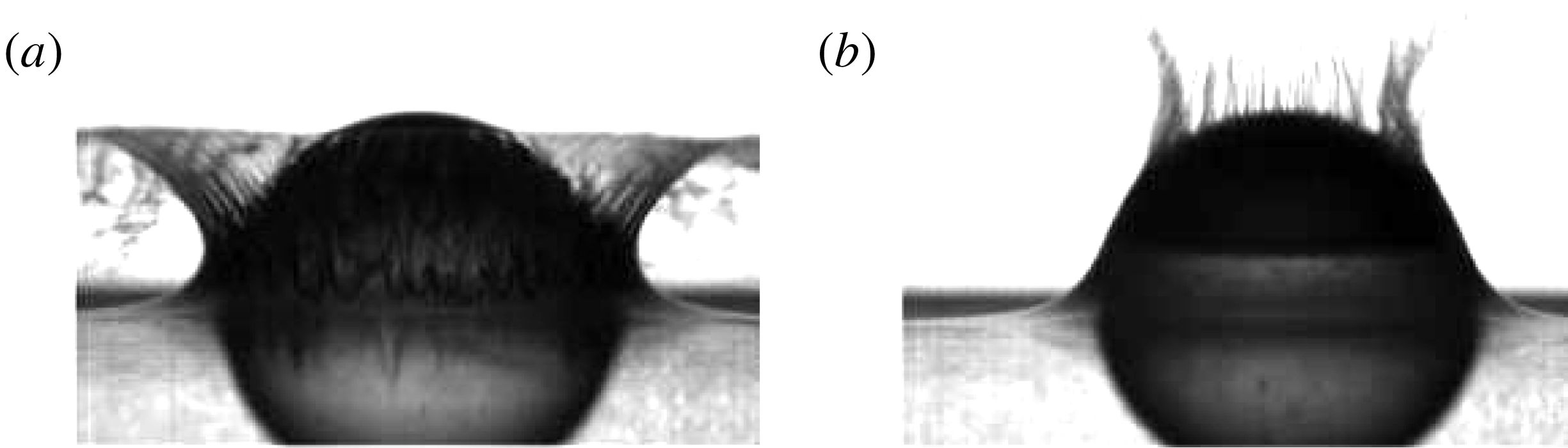
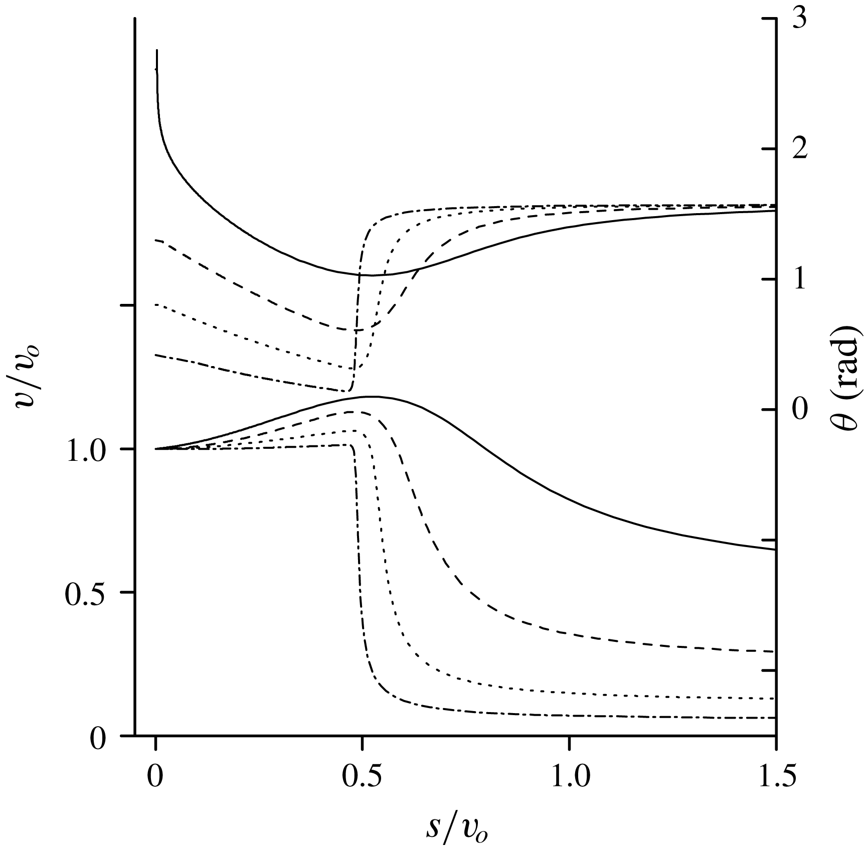
When a solid body penetrates through a liquid surface, it is common to see that the liquid will move along the body surface initially and then depart from the body surface, especially when the body surface has curvature and the entry speed is relatively large. However, it was found by Duez et al. (Reference Duez, Ybert, Clanet and Bocquet2007) that for two identical bodies, when a different nanometric coating leading a different wettability was applied on the body surface, different fluid flow behaviours could be observed (see figure 1).
For a hydrophobic body, flow would indeed depart from the body surface, while for a hydrophilic body, the fluid will keep moving along the body surface when the entry speed is below a critical speed. This presents a major challenge in mathematical modelling of the water entry problem. In fact, within the framework of inviscid flow, the impermeable condition is commonly used on a solid surface. This means that on the body surface, its normal velocity is the same as that of the fluid particle at the same point. In other words, the direction of fluid particle velocity will be tangential to the body surface. The challenge that it then presents to mathematical modelling and numerical simulations is that at each time step the fluid particle at the intersection of the free surface and the body surface can move at the next time step along the body surface or depart the body surface tangentially. In either case, the impermeable condition at the intersection point holds. However, in the former case, the flow remains attached to the body surface, while in the latter case, the flow becomes detached from the body surface. The subsequent flow configurations and pressure distribution in the two cases are expected to be different.
Impacting spheres with two different wettabilities at the same impact velocity:(a) hydrophobic sphere and (b) hydrophilic sphere. Adopted from Duez et al. (Reference Duez, Ybert, Clanet and Bocquet2007).

Much of the work on water entry has been focusing on the attached flow, especially for a body without curvature, namely a wedge. At the early stage of impact or when the gravity effect is ignored, the velocity potential flow problem for such a body geometry becomes self-similar. A complete nonlinear solution was obtained by Dobrovol’skaya (Reference Dobrovol’skaya1969) using the theory of complex functions and mapping technique for a symmetric wedge entry. Using an integral hodograph method, Semenov & Iafrati (Reference Semenov and Iafrati2006) and Semenov & Yoon (Reference Semenov and Yoon2009) solved the problem for water entry of an asymmetric wedge. This nonlinear water entry problem of a wedge was also solved through the boundary element method by Xu, Duan & Wu (Reference Xu, Duan and Wu2008). Another popular technique in the water entry problem is the Wagner method (Wagner Reference Wagner1932). He introduced a correction in the method of von Karman (Reference von Karman1929) who assumed that the free surface remained flat and the potential on the free surface was zero during impact, and the two-dimensional body below the free surface could be replaced by a flat plate with the length equal to the distance between the two intersections of the body surface and the undisturbed free surface. After Wagner’s correction, the length of the plate included the effect of the local free surface elevation, and therefore, the length itself was the part the solution. However, jet developed along the body surface during the impact was ignored. The Wagner theory was further improved and extended based on a matched asymptotic expansion method. In particular, the jets attached on the body were taken into consideration without flow detachment (Armand & Cointe Reference Armand and Cointe1987; Howison, Ockendon & Wilson Reference Howison, Ockendon and Wilson1991; Howison, Ockendon & Oliver Reference Howison, Ockendon and Oliver2002, Reference Howison, Ockendon and Oliver2004; Korobkin Reference Korobkin2004; Moore et al. Reference Moore, Ockendon, Ockendon and Oliver2015). Unlike the fully nonlinear theory for the self-similar flow, Wagner theory is not limited to a body with no curvature.
There has also been some work on water entry with flow detachment and splash jets for a body with a sharp corner. This includes a wedge of finite height, which was considered by Zhao, Faltinsen & Aarsnes (Reference Zhao, Faltinsen and Aarsnes1997). The fluid particle would depart the body surface when it reached the knuckle of the body. The work was extended by Sun & Faltinsen (Reference Sun and Faltinsen2007) to a planing vessel. Tassin, Korobkin, & Cooker (Reference Tassin, Korobkin and Cooker2014) used an analytical model based on the Logvinovich (Logvinovich Reference Logvinovich1969) model for water entry of a finite wedge with flow detachment. Sun & Faltinsen (Reference Sun and Faltinsen2009) simulated a finite bow-flare section with roll angle vertically entering the calm water. Bao, Wu & Xu (Reference Bao, Wu and Xu2016) considered water entry of a finite wedge with flow detachment at a prescribed velocity while Bao, Wu & Xu (Reference Bao, Wu and Xu2017) further considered free fall motion.
As the above work is noticeably about a body with a sharp corner, the point of detachment is assumed to be at the corner. To stay on the body surface, the flow would have to change direction sharply, leading to an infinite velocity and pressure gradient or acceleration. The determination of the detachment point for a curved body is obviously more complex, especially for what has been observed by Duez et al. (Reference Duez, Ybert, Clanet and Bocquet2007) for hydrophobic and hydrophilic bodes. In this study, we consider the nonlinear problem of the cylindrical curved body entering the undisturbed flat free surface. In order for the problem to be solved within the framework of self-similar flow, the cylinder is assumed to stretch at the same time it enters water. It should be noted that using an expanding body to undertake depth analysis for a water entry problem is not unusual. In fact, in Wagner’s theory, the width of the equivalent plate is continuously stretching. Wu & Sun (Reference Wu and Sun2014) investigated an attached flow for an expanding three-dimensional paraboloid. Semenov & Wu (Reference Semenov and Wu2016) considered a stretching finite wedge. In the latter work, at the moment of impact, the tip of the jet coincides with the wedge apex and then starts moving along the wedge surface. If its speed is larger than the stretching speed of the wedge, the flow will depart from the body and form the splash jet. In such a case, the distance between the tip of the splash jet and the knuckle of the wedge,
 $l_{jet}$
, can be considered as the parameter of the solution. Using this parameter, it is then obvious when
 $l_{jet}=0$
, the detached flow has become the attached one. We can then use this parameter for the current curved body. Within the framework of self-similar flow, for each case of water entry, we will seek both solutions corresponding to
 $l_{jet}>0$
and
 $l_{jet}=0$
, which correspond to hydrophobic and hydrophilic bodies, respectively. We shall then investigate the features in both detached and attached flows, including flow pattern, pressure distribution and free surface including splash jet. For the case of detached flow with
 $l_{jet}>0$
, the point of detachment will be determined by the requirement for continuity and finite spatial derivative of the velocity at the point. We also show that in such a case, the Brillouin–Villat condition (Villat Reference Villat1914) holds at the point of detachment, as in the similar steady flow problem (Semenov & Wu Reference Semenov and Wu2013).
The problem of the expanding body entering the free surface may look artificial. However, it does have some practical relevance. It can be applied to model a strong gas explosion occurring near the free surface at the initial time Sedov (Reference Sedov1993). The model of an expanding body may be also relevant to the hydrodynamic analysis of fast ships or dicing aircraft within the framework of the so-called
 $2D+t$
approach Faltinsen (Reference Faltinsen2005), Climent et al. (Reference Climent, Benitez, Rosich, Rueda and Pentecote2006), Tassin et al. (Reference Tassin, Korobkin and Cooker2014). There the ship is divided into many transverse sections along the longitudinal direction. The fluid flow problem is solved by a two-dimensional theory section by section from the bow. As the area of the cross section of the ship increases its size towards its middle part, it is equivalent to expansion in the
 $2D$
theory. When the shape of the section is the same and its typical length increases longitudinally, the flow in the
 $2D$
theory may become self similar when the gravity effect is ignored.
The solutions for both detached and attached flows will be found through the integral hodograph method (Semenov & Cummings Reference Semenov and Cummings2006). It is based on the implicit conformal mapping through the derivation of analytical expressions for the complex velocity potential, the conjugate of complex velocity and the mapping function in the first quadrant of a parameter plane. The original boundary value problem is converted to a system of integro-differential equations in terms of the velocity magnitude and the velocity angle relative to the liquid boundary. They are solved numerically using the method of successive approximations. The results are presented in terms of pressure distribution, free surface shape and streamlines and tip angle of the splash jet.
2 Formulation of the problem and the solution methodology
We consider an arbitrary shaped body, which expands with speed
 $U$
in time in a self-similar way and enters into the liquid of infinite depth such that velocity of the bottom point is
 $V$
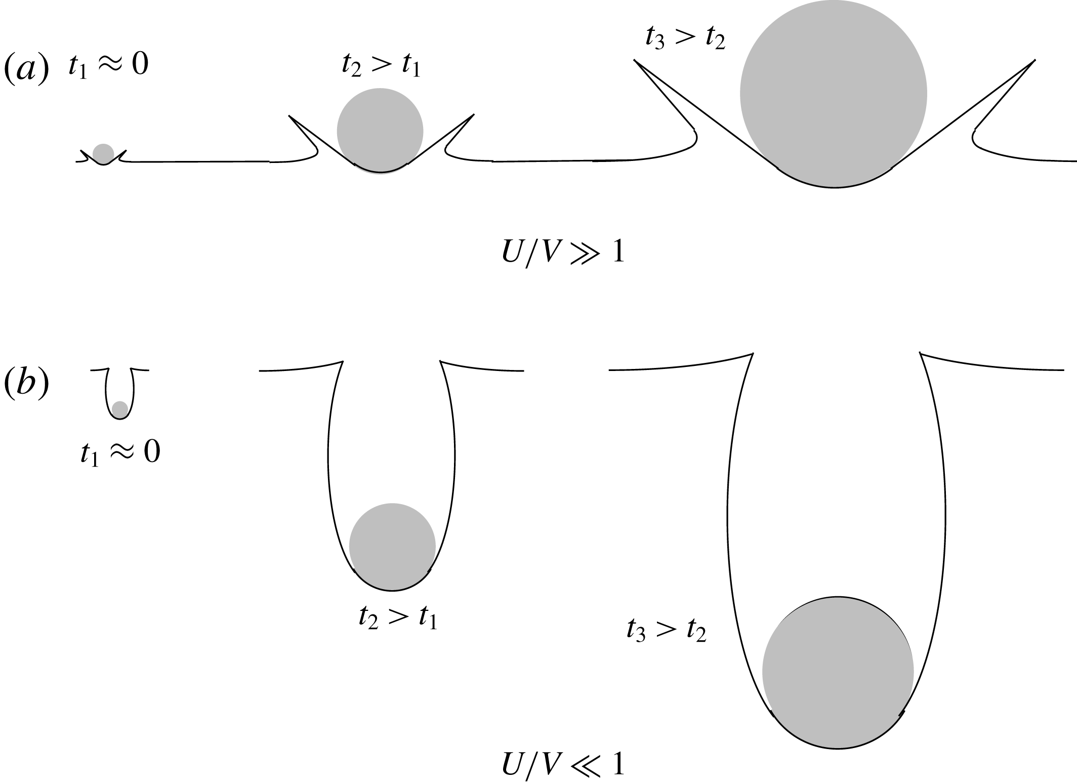
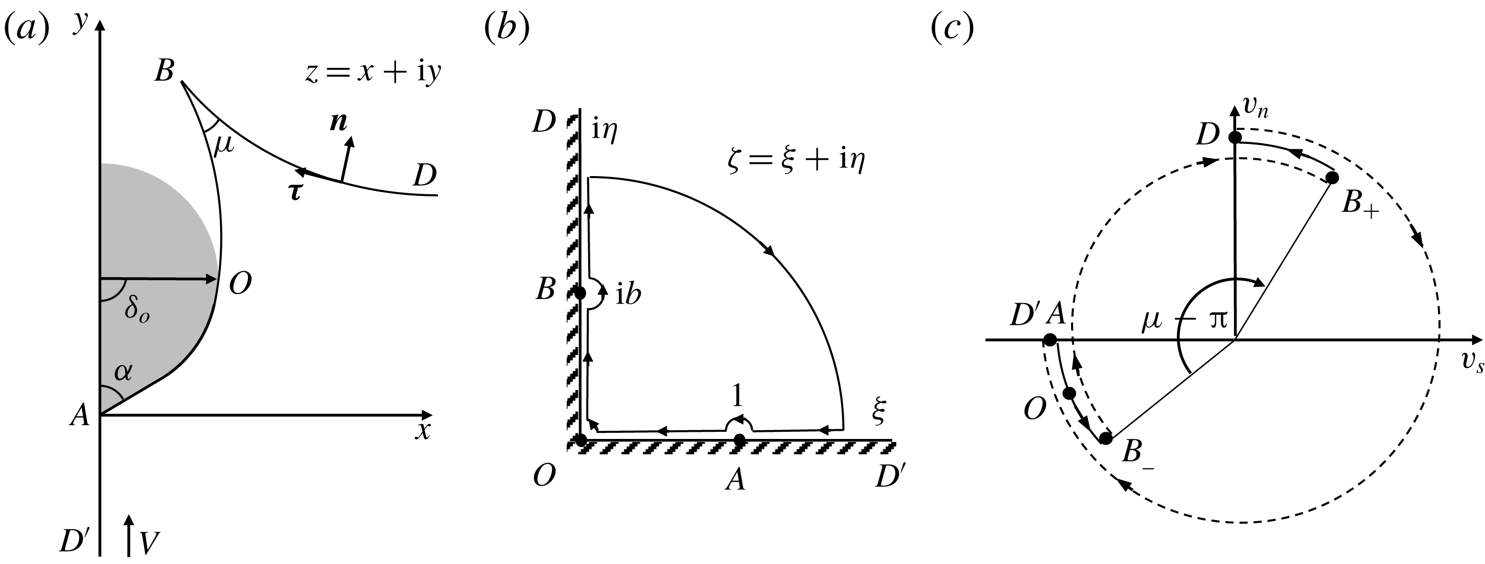
directed into the liquid. The body starts from a single point on the free surface and then its typical length expands linearly in time as shown in figure 2. Based on the dynamic equivalence, the formulation of the problem will be considered in the system of Cartesian coordinates
 $X,Y$
with the origin at the bottom point of the body, in which the flow comes from
 $Y=-\infty$
with velocity
 $V$
. The body shape is given as
 $Y_{b}(X,t)=Vty_{b}(x)$
, where
 $x=X/Vt$
and
 $y=Y/Vt$
are the self-similar variables.
The statement of the problem can be formulated as follows. We have to determine the complex potential of the flow,
 $W(Z,t)$
, which satisfies an impermeable boundary condition on the expanding body surface and the nonlinear dynamic boundary condition on the free surface.
Flow development as time in progress for (a) fast expansion and (b) slow expansion.

The complex plane
 $Z$
in the physical plane can be written in terms of the self-similar variables as
 $$\begin{eqnarray}\displaystyle Z=Vtz, & & \displaystyle\end{eqnarray}$$
with
 $z=x+\text{i}y$
. In this self-similar complex plane
 $z$
, the free surface and the shape of the body,
 $y_{b}=y_{b}(x)$
, are stationary. Correspondingly, the complex-velocity potential
 $W(Z,t)$
in the physical plane for the self-similar flow can be written as
 $$\begin{eqnarray}\displaystyle W(Z,t)=\unicode[STIX]{x1D6F7}(X,Y,t)+\text{i}\unicode[STIX]{x1D6F9}(X,Y,t)=V^{2}t[\unicode[STIX]{x1D719}(x,y)+\text{i}\unicode[STIX]{x1D713}(x,y)], & & \displaystyle\end{eqnarray}$$
where
 $\unicode[STIX]{x1D719}$
and
 $\unicode[STIX]{x1D713}$
are the velocity potential and the stream function, respectively.
The problem is to determine the function
 $w(z)$
, which conformally maps the self-similar or stationary plane
 $z$
, onto the complex-velocity potential region
 $w$
. We shall use the integral hodograph method (Semenov & Cummings Reference Semenov and Cummings2006). In the method, a parameter plane
 $\unicode[STIX]{x1D701}$
is introduced as suggested by Joukovskii (Reference Joukovskii1890) and Michell (Reference Michell1890). Instead of finding
 $w(z)$
directly, two complex functions,
 $\text{d}w/\text{d}z$
, which are the conjugate of the complex velocity and will be referred to as the complex velocity subsequently, and the function
 $\text{d}w/\text{d}\unicode[STIX]{x1D701}$
are both sought in the
 $\unicode[STIX]{x1D701}$
-plane in integral form. Once these two functions are found, the relation between the parameter and stationary planes can be determined as follows:
 $$\begin{eqnarray}\displaystyle z(\unicode[STIX]{x1D701})=z_{0}+\int _{0}^{\unicode[STIX]{x1D701}}\frac{\text{d}z}{\text{d}\unicode[STIX]{x1D701}}\,\text{d}\unicode[STIX]{x1D701}=\int _{0}^{\unicode[STIX]{x1D701}}\left.\frac{\text{d}w}{\text{d}\unicode[STIX]{x1D701}}\right/\frac{\text{d}w}{\text{d}z}\,\text{d}\unicode[STIX]{x1D701}, & & \displaystyle\end{eqnarray}$$
where
 $z_{0}=z(\unicode[STIX]{x1D701})_{\unicode[STIX]{x1D701}=0}$
.
(a) The similarity plane
 $z=x+\text{i}y$
for a flow with velocity
 $V$
impacting an expanding body. (b) The
 $\unicode[STIX]{x1D701}$
-plane where arrows in the closed line show the path of integration in (2.9), which is opposite to the direction of vector
 $\unicode[STIX]{x1D749}$
, the arc length coordinate
 $s$
and (c) variation of the velocity angle
 $\unicode[STIX]{x1D714}=\arg (v_{s}+\text{i}v_{n})$
to the whole boundary of the flow domain. Its continuous and step variations are shown by solid lines and dashed lines, respectively. Points
 $A,O,B_{-},B_{+}$
and
 $D$
are marked through solid points and the route follows
 $D^{\prime },A,O,B_{-},B_{+},D$
. When the body is smooth at point
 $A$
, the angle
 $\unicode[STIX]{x1D6FC}=\unicode[STIX]{x03C0}/2$
.

Based on the method of Chaplygin (see 5 of chap. 1 in Gurevich (Reference Gurevich1965)) we choose the first quadrant of the
 $\unicode[STIX]{x1D701}$
-plane shown in figure 3(b) as the parameter region, which corresponds to the flow region of
 $x\geqslant 0$
in the stationary plane in figure 3(a). The functions
 $\text{d}w/\text{d}z$
and
 $\text{d}w/\text{d}\unicode[STIX]{x1D701}$
conformally map the parameter region onto the regions of the complex velocity and the derivative of the complex potential. Based on the theorem of conformal mapping, three points in the parameter plane can be chosen, which are taken as
 $O$
(intersection point of the body surface and the free surface),
 $D$
(a point at infinity) and
 $A$
(stagnation point at the bottom of the body), as shown in figure 3(b). In the parameter plane, the interval
 $0\leqslant \unicode[STIX]{x1D702}\leqslant b$
of the imaginary axis corresponds to the free surface from the intersection point
 $O$
to the tip of the splash jet
 $B$
and the interval
 $b\leqslant \unicode[STIX]{x1D702}\leqslant \infty$
corresponds to the main free surface
 $BD$
. The interval
 $0\leqslant \unicode[STIX]{x1D709}\leqslant 1$
of the real axis corresponds to the wetted surface of the body, and the rest of the positive real axis (
 $1\leqslant \unicode[STIX]{x1D709}\leqslant \infty$
) corresponds to the symmetry line
 $AD^{\prime }$
. The parameter
 $b$
is unknown and will be discussed. In order to determine the functions
 $\text{d}w/\text{d}z$
and
 $\text{d}w/\text{d}\unicode[STIX]{x1D701}$
, we shall formulate appropriate boundary-value problems for each of these functions in the
 $\unicode[STIX]{x1D701}$
-plane.
2.1 Expression for the complex velocity,
 $\text{d}w/\text{d}z$

At this stage, we denote the angle of the velocity direction along the body as
 $\unicode[STIX]{x1D6FD}(\unicode[STIX]{x1D709})$
and the velocity magnitude on the free surface as
 $v(\unicode[STIX]{x1D702})$
. With these notations, we have the following boundary conditions for the function
 $\text{d}w/\text{d}z$
in the first quadrant of the
 $\unicode[STIX]{x1D701}$
-plane:
 $$\begin{eqnarray}\displaystyle & \displaystyle \unicode[STIX]{x1D712}(\unicode[STIX]{x1D709})=\arg \left(\frac{\text{d}w}{\text{d}z}\right)=\left\{\begin{array}{@{}ll@{}}-\unicode[STIX]{x1D6FD}(\unicode[STIX]{x1D709}), & 0\leqslant \unicode[STIX]{x1D709}\leqslant 1,\\ -\unicode[STIX]{x03C0}/2, & 1\leqslant \unicode[STIX]{x1D709}<\infty ,\end{array}\right. & \displaystyle\end{eqnarray}$$
 $$\begin{eqnarray}\displaystyle & \displaystyle v(\unicode[STIX]{x1D702})=\left|\frac{\text{d}w}{\text{d}z}\right|_{\unicode[STIX]{x1D701}=i\unicode[STIX]{x1D702}},\quad 0\leqslant \unicode[STIX]{x1D702}<\infty . & \displaystyle\end{eqnarray}$$
The complex velocity can be written in the following integral formula (Semenov & Cummings Reference Semenov and Cummings2006; Semenov & Iafrati Reference Semenov and Iafrati2006):
 $$\begin{eqnarray}\displaystyle \frac{\text{d}w}{\text{d}z}=v_{\infty }\exp \left[\frac{1}{\unicode[STIX]{x03C0}}\int _{0}^{\infty }\frac{\text{d}\unicode[STIX]{x1D712}}{\text{d}\unicode[STIX]{x1D709}}\ln \left(\frac{\unicode[STIX]{x1D701}+\unicode[STIX]{x1D709}}{\unicode[STIX]{x1D701}-\unicode[STIX]{x1D709}}\right)\text{d}\unicode[STIX]{x1D709}-\frac{\text{i}}{\unicode[STIX]{x03C0}}\int _{0}^{\infty }\frac{\text{d}\ln v}{\text{d}\unicode[STIX]{x1D702}}\ln \left(\frac{\unicode[STIX]{x1D701}-\text{i}\unicode[STIX]{x1D702}}{\unicode[STIX]{x1D701}+\text{i}\unicode[STIX]{x1D702}}\right)\text{d}\unicode[STIX]{x1D702}+\text{i}\unicode[STIX]{x1D712}_{\infty }\right]. & & \displaystyle \nonumber\\ \displaystyle & & \displaystyle\end{eqnarray}$$
In (2.6), the velocity at point
 $D$
or
 $\unicode[STIX]{x1D701}\rightarrow \infty$
,
 $v_{\infty }=1$
, as
 $V$
, the incoming velocity at infinity has been chosen as the reference velocity, and
 $\unicode[STIX]{x1D712}_{\infty }=-\unicode[STIX]{x03C0}/2$
as
 $D^{\prime }$
on the symmetry line
 $AD^{\prime }$
. The function
 $\unicode[STIX]{x1D712}(\unicode[STIX]{x1D709})$
, which is related to the velocity direction, has a jump of
 $\unicode[STIX]{x0394}\unicode[STIX]{x1D712}_{A}=\unicode[STIX]{x1D6FC}$
when passing point
 $A$
from
 $D^{\prime }A$
line to
 $AO$
line, since it is equal to
 $-\unicode[STIX]{x03C0}/2$
on
 $D^{\prime }A$
and
 $\unicode[STIX]{x1D6FD}(\unicode[STIX]{x1D709})\rightarrow \unicode[STIX]{x03C0}/2-\unicode[STIX]{x1D6FC}$
as
 $\unicode[STIX]{x1D709}\rightarrow 1-\unicode[STIX]{x1D716}$
, where
 $\unicode[STIX]{x1D716}\rightarrow 0$
. Using (2.4) and evaluating the integral of the function
 $\unicode[STIX]{x1D712}(\unicode[STIX]{x1D709})$
over the jump, equation (2.6) becomes
 $$\begin{eqnarray}\displaystyle \frac{\text{d}w}{\text{d}z} & = & \displaystyle v_{0}\left(\frac{\unicode[STIX]{x1D701}-1}{\unicode[STIX]{x1D701}+1}\right)^{\unicode[STIX]{x1D6FC}/\unicode[STIX]{x03C0}}\exp \left[\frac{1}{\unicode[STIX]{x03C0}}\int _{0}^{1}\frac{\text{d}\unicode[STIX]{x1D6FD}}{\text{d}\unicode[STIX]{x1D709}}\ln \left(\frac{\unicode[STIX]{x1D709}-\unicode[STIX]{x1D701}}{\unicode[STIX]{x1D709}+\unicode[STIX]{x1D701}}\right)\text{d}\unicode[STIX]{x1D709}\right.\nonumber\\ \displaystyle & & \displaystyle -\left.\frac{\text{i}}{\unicode[STIX]{x03C0}}\int _{0}^{\infty }\frac{\text{d}\ln v}{\text{d}\unicode[STIX]{x1D702}}\ln \left(\frac{\text{i}\unicode[STIX]{x1D702}-\unicode[STIX]{x1D701}}{\text{i}\unicode[STIX]{x1D702}+\unicode[STIX]{x1D701}}\right)\text{d}\unicode[STIX]{x1D702}-\text{i}(\unicode[STIX]{x1D6FD}_{0}+\unicode[STIX]{x1D6FC})\right],\end{eqnarray}$$
where
 $\unicode[STIX]{x1D6FD}_{0}=\unicode[STIX]{x1D6FD}(\unicode[STIX]{x1D709})_{\unicode[STIX]{x1D709}=0}$
and
 $v_{0}=v(\unicode[STIX]{x1D702})_{\unicode[STIX]{x1D702}=0}$
are their corresponding values at point
 $O$
. The functions
 $\unicode[STIX]{x1D6FD}(\unicode[STIX]{x1D709})$
and
 $v(\unicode[STIX]{x1D702})$
will be determined later from the kinematic and dynamic boundary conditions. When the body is smooth at point
 $A$
, the angle
 $\unicode[STIX]{x1D6FC}=\unicode[STIX]{x03C0}/2$
.
2.2 Expression for the derivative of the complex potential,
$\text{d}w/\text{d}\unicode[STIX]{x1D701}$

In order to obtain the expression for the derivative of the complex potential, it is useful to introduce the unit vectors
 $\boldsymbol{n}$
and
 $\unicode[STIX]{x1D749}$
on the fluid boundary, which are normal and tangential to the boundary, respectively. The former is directed outwards from the liquid region, and while one moves in the latter direction along the boundary, the arc length coordinate
 $s$
increases and the liquid region is on the left hand side (see figure 3
a). With these notations, we have
 $$\begin{eqnarray}\displaystyle \text{d}w=(v_{s}+\text{i}v_{n})\,\text{d}s=v\text{e}^{\text{i}\unicode[STIX]{x1D714}}\,\text{d}s, & & \displaystyle\end{eqnarray}$$
where
 $\unicode[STIX]{x1D714}(\unicode[STIX]{x1D701})=\arg (v_{s}+\text{i}v_{n})$
,
 $v_{n}$
and
 $v_{s}$
are the normal and tangential velocity components, respectively. Variation of the function
 $\unicode[STIX]{x1D714}(\unicode[STIX]{x1D701})$
along the entire boundary of the flow region is shown in figure 3(c). The arrows in figure 3(b) show the clockwise direction of the boundary. Along this direction
 $\unicode[STIX]{x1D714}(\unicode[STIX]{x1D701})_{\unicode[STIX]{x1D701}=\unicode[STIX]{x1D709}}=-\unicode[STIX]{x03C0}$
from
 $\unicode[STIX]{x1D709}\rightarrow \infty$
to
 $\unicode[STIX]{x1D709}=1$
or from
 $D^{\prime }$
to
 $A$
, since
 $v_{n}=0$
and
 $v_{s}<0$
, and
 $\unicode[STIX]{x1D714}(\unicode[STIX]{x1D701})_{\unicode[STIX]{x1D701}=\unicode[STIX]{x1D709}}=\unicode[STIX]{x1D6FE}(\unicode[STIX]{x1D709})$
from
 $\unicode[STIX]{x1D709}=1$
to
 $\unicode[STIX]{x1D709}=0$
, or from
 $A$
to
 $O$
corresponding to the wetted surface of the body.
 $\unicode[STIX]{x1D714}(\unicode[STIX]{x1D701})_{\unicode[STIX]{x1D701}=\text{i}\unicode[STIX]{x1D702}}=\unicode[STIX]{x1D703}(\unicode[STIX]{x1D702})$
on the free surface changes continuously along
 $OB$
and
 $BD$
, or in the intervals
 $(0,b)$
and
 $(b,\infty )$
on the
 $\unicode[STIX]{x1D702}$
-axis. At point
 $B$
 $\unicode[STIX]{x1D703}(\unicode[STIX]{x1D702})$
has a jump of
 $\unicode[STIX]{x1D6E5}_{B}=-\unicode[STIX]{x03C0}+\unicode[STIX]{x1D707}$
from
 $B_{-}$
to
 $B_{+}$
, where
 $\unicode[STIX]{x1D707}$
is the angle of the jet tip at point
 $B$
, as defined previously. Based on the above analysis, we can write the function
 $\unicode[STIX]{x1D714}(\unicode[STIX]{x1D701})$
as follows
 $$\begin{eqnarray}\displaystyle \unicode[STIX]{x1D714}(\unicode[STIX]{x1D701})=\arg \left(\frac{\text{d}w}{\text{d}s}\right)=\left\{\begin{array}{@{}ll@{}}-\unicode[STIX]{x03C0}, & 1\leqslant \unicode[STIX]{x1D709}<\infty ,\quad \unicode[STIX]{x1D702}=0,\\ \unicode[STIX]{x1D6FE}, & 0\leqslant \unicode[STIX]{x1D709}\leqslant 1,\quad \unicode[STIX]{x1D702}=0,\\ \unicode[STIX]{x1D706}(\unicode[STIX]{x1D702}), & \unicode[STIX]{x1D709}=0,0\leqslant \unicode[STIX]{x1D702}\leqslant b,\\ \unicode[STIX]{x1D706}(\unicode[STIX]{x1D702})+\unicode[STIX]{x1D6E5}_{B}, & \unicode[STIX]{x1D709}=0,b\leqslant \unicode[STIX]{x1D702}<\infty ,\end{array}\right. & & \displaystyle\end{eqnarray}$$
where
 $\unicode[STIX]{x1D706}(\unicode[STIX]{x1D702})$
is a continuous function. Equation (2.9) allows us to determine the argument of the derivative of the complex potential
 $$\begin{eqnarray}\displaystyle \unicode[STIX]{x1D717}(\unicode[STIX]{x1D701})=\arg \left(\frac{\text{d}w}{\text{d}\unicode[STIX]{x1D701}}\right)=\arg \left(\frac{\text{d}w}{\text{d}s}\right)+\arg \left(\frac{\text{d}s}{\text{d}\unicode[STIX]{x1D701}}\right)=\unicode[STIX]{x1D714}(\unicode[STIX]{x1D701})+\left\{\begin{array}{@{}ll@{}}0, & 0<\unicode[STIX]{x1D709}<\infty ,\quad \unicode[STIX]{x1D702}=0,\\ \unicode[STIX]{x03C0}/2, & \unicode[STIX]{x1D709}=0,0<\unicode[STIX]{x1D702}<\infty .\end{array}\right. & & \displaystyle \nonumber\\ \displaystyle & & \displaystyle\end{eqnarray}$$
The function
 $\unicode[STIX]{x1D706}(\unicode[STIX]{x1D702})$
varies from
 $\unicode[STIX]{x1D706}_{0}=\unicode[STIX]{x1D703}(\unicode[STIX]{x1D702})_{\unicode[STIX]{x1D702}=0}=\unicode[STIX]{x1D6FE}(\unicode[STIX]{x1D709})_{\unicode[STIX]{x1D709}=0}$
at point
 $O$
to
 $\unicode[STIX]{x1D706}_{\infty }=\unicode[STIX]{x1D706}(\unicode[STIX]{x1D702})_{\unicode[STIX]{x1D702}\rightarrow \infty }=\unicode[STIX]{x1D703}_{\infty }+\unicode[STIX]{x03C0}-\unicode[STIX]{x1D707}$
at point
 $D$
. Since
 $\unicode[STIX]{x1D703}_{\infty }=\unicode[STIX]{x1D703}_{D}=\unicode[STIX]{x03C0}/2$
, because the velocity direction at infinity is perpendicular to the free surface, the angle
 $\unicode[STIX]{x1D707}$
can be determined from
 $\unicode[STIX]{x1D707}=(3/2)\unicode[STIX]{x03C0}-\unicode[STIX]{x1D706}_{\infty }$
.
The derivative of the potential can be written in the following integral formula (Semenov & Cummings Reference Semenov and Cummings2006; Semenov & Iafrati Reference Semenov and Iafrati2006):
 $$\begin{eqnarray}\displaystyle \frac{\text{d}w}{\text{d}\unicode[STIX]{x1D701}}=K\exp \left[\frac{1}{\unicode[STIX]{x03C0}}\int _{\infty }^{0}\frac{\text{d}\unicode[STIX]{x1D717}}{\text{d}\unicode[STIX]{x1D709}}\ln (\unicode[STIX]{x1D701}^{2}-\unicode[STIX]{x1D709}^{2})\,\text{d}\unicode[STIX]{x1D709}+\frac{1}{\unicode[STIX]{x03C0}}\int _{0}^{\infty }\frac{\text{d}\unicode[STIX]{x1D717}}{\text{d}\unicode[STIX]{x1D702}}\ln (\unicode[STIX]{x1D701}^{2}+\unicode[STIX]{x1D702}^{2})\,\text{d}\unicode[STIX]{x1D702}+\text{i}\unicode[STIX]{x1D717}_{\infty }\right], & & \displaystyle\end{eqnarray}$$
where
 $K$
is a real factor and
 $\unicode[STIX]{x1D717}_{\infty }=\unicode[STIX]{x1D717}(\unicode[STIX]{x1D701})_{|\unicode[STIX]{x1D701}|\rightarrow \infty }$
. By substituting (2.9) and (2.10) into (2.11) and evaluating the integrals over each step change of the function
 $\unicode[STIX]{x1D717}(\unicode[STIX]{x1D701})$
, we obtain
 $$\begin{eqnarray}\displaystyle \frac{\text{d}w}{\text{d}\unicode[STIX]{x1D701}} & = & \displaystyle K\unicode[STIX]{x1D701}(b^{2}+\unicode[STIX]{x1D701}^{2})^{\unicode[STIX]{x1D707}/\unicode[STIX]{x03C0}-1}\exp \left[-\frac{1}{\unicode[STIX]{x03C0}}\int _{0}^{1}\frac{\text{d}\unicode[STIX]{x1D6FE}}{\text{d}\unicode[STIX]{x1D709}}\ln (\unicode[STIX]{x1D709}^{2}-\unicode[STIX]{x1D701}^{2})\,\text{d}\unicode[STIX]{x1D709}\right.\nonumber\\ \displaystyle & & \displaystyle +\left.\frac{1}{\unicode[STIX]{x03C0}}\int _{0}^{\infty }\frac{\text{d}\unicode[STIX]{x1D706}}{\text{d}\unicode[STIX]{x1D702}}\ln (\unicode[STIX]{x1D701}^{2}+\unicode[STIX]{x1D702}^{2})\,\text{d}\unicode[STIX]{x1D702}+\text{i}\unicode[STIX]{x1D6FE}_{0}\right].\end{eqnarray}$$
The integration of this equation with respect to
 $\unicode[STIX]{x1D701}$
gives the complex potential
 $w(\unicode[STIX]{x1D701})$
as
 $$\begin{eqnarray}\displaystyle w(\unicode[STIX]{x1D701}) & = & \displaystyle w_{A}+K\int _{1}^{\unicode[STIX]{x1D701}}\unicode[STIX]{x1D701}^{\prime }(\unicode[STIX]{x1D701}^{\prime ^{2}}+b^{2})^{\unicode[STIX]{x1D707}/\unicode[STIX]{x03C0}-1}\exp \left[-\frac{1}{\unicode[STIX]{x03C0}}\int _{0}^{1}\frac{\text{d}\unicode[STIX]{x1D6FE}}{\text{d}\unicode[STIX]{x1D709}}\ln (\unicode[STIX]{x1D709}^{2}-\unicode[STIX]{x1D701}^{\prime ^{2}})\,\text{d}\unicode[STIX]{x1D709}\right.\nonumber\\ \displaystyle & & \displaystyle +\left.\frac{1}{\unicode[STIX]{x03C0}}\int _{0}^{\infty }\frac{\text{d}\unicode[STIX]{x1D706}}{\text{d}\unicode[STIX]{x1D702}}\ln (\unicode[STIX]{x1D701}^{\prime ^{2}}+\unicode[STIX]{x1D702}^{2})\,\text{d}\unicode[STIX]{x1D702}+\text{i}\unicode[STIX]{x1D6FE}_{0}\right]\text{d}\unicode[STIX]{x1D701}^{\prime },\end{eqnarray}$$
where
 $w_{A}=w(\unicode[STIX]{x1D701})_{\unicode[STIX]{x1D701}=1}$
. From (2.7) and (2.12), the derivative of the mapping function from the parameter plane to the similarity plane can be obtained as
 $$\begin{eqnarray}\displaystyle \frac{\text{d}z}{\text{d}\unicode[STIX]{x1D701}} & = & \displaystyle \frac{K\unicode[STIX]{x1D701}}{v_{0}}(\unicode[STIX]{x1D701}^{2}+b^{2})^{\unicode[STIX]{x1D707}/\unicode[STIX]{x03C0}-1}\left(\frac{\unicode[STIX]{x1D701}+1}{\unicode[STIX]{x1D701}-1}\right)^{\unicode[STIX]{x1D6FC}/\unicode[STIX]{x03C0}}\nonumber\\ \displaystyle & & \displaystyle \times \exp \left[-\frac{1}{\unicode[STIX]{x03C0}}\int _{0}^{1}\frac{\text{d}\unicode[STIX]{x1D6FE}}{\text{d}\unicode[STIX]{x1D709}}\ln (\unicode[STIX]{x1D709}^{2}-\unicode[STIX]{x1D701}^{2})\,\text{d}\unicode[STIX]{x1D709}+\frac{1}{\unicode[STIX]{x03C0}}\int _{0}^{\infty }\frac{\text{d}\unicode[STIX]{x1D706}}{\text{d}\unicode[STIX]{x1D702}}\ln (\unicode[STIX]{x1D702}^{2}+\unicode[STIX]{x1D701}^{2})\,\text{d}\unicode[STIX]{x1D702}\right.\nonumber\\ \displaystyle & & \displaystyle -\,\frac{1}{\unicode[STIX]{x03C0}}\int _{0}^{1}\frac{\text{d}\unicode[STIX]{x1D6FD}}{\text{d}\unicode[STIX]{x1D709}}\ln \left(\frac{\unicode[STIX]{x1D709}-\unicode[STIX]{x1D701}}{\unicode[STIX]{x1D709}+\unicode[STIX]{x1D701}}\right)\text{d}\unicode[STIX]{x1D709}\nonumber\\ \displaystyle & & \displaystyle +\left.\frac{\text{i}}{\unicode[STIX]{x03C0}}\int _{0}^{\infty }\frac{\text{d}\ln v}{\text{d}\unicode[STIX]{x1D702}}\ln \left(\frac{\text{i}\unicode[STIX]{x1D702}-\unicode[STIX]{x1D701}}{\text{i}\unicode[STIX]{x1D702}+\unicode[STIX]{x1D701}}\right)\text{d}\unicode[STIX]{x1D702}+\text{i}(\unicode[STIX]{x1D6FD}_{0}+\unicode[STIX]{x1D6FE}_{0}+\unicode[STIX]{x1D6FC})\right].\end{eqnarray}$$
Integration of the above equation with respect to
 $\unicode[STIX]{x1D701}$
yields the mapping function
 $z=z(\unicode[STIX]{x1D701})$
.
We notice that point
 $B$
is initiated from point
 $A$
at time
 $t=0$
. For the self-similar flow, the velocity of point
 $B$
will be always
 $Vv_{B}\text{e}^{\text{i}\unicode[STIX]{x1D6FD}_{B}}$
and its position in the physical plane will be
 $Z_{B}=Vtv_{B}\text{e}^{\text{i}\unicode[STIX]{x1D6FD}_{B}}$
, which gives
 $z_{B}=v_{B}\text{e}^{\text{i}\unicode[STIX]{x1D6FD}_{B}}$
based on (2.1). Thus we have
 $$\begin{eqnarray}\displaystyle |z_{B}|=v_{B}, & & \displaystyle\end{eqnarray}$$
from which the parameter
 $K$
is determined. Here,
 $z_{B}$
is obtained by integration of the derivative of the mapping function (2.14) along the imaginary axis of the parameter plane in the interval (
 $0\leqslant \unicode[STIX]{x1D702}\leqslant b$
), and the velocity at the tip of the splash jet is
 $v_{B}=v(\unicode[STIX]{x1D702})_{\unicode[STIX]{x1D702}=b}$
. When (2.15) is satisfied,
 $\arg z_{B}=\unicode[STIX]{x1D6FD}_{B}$
can be automatically satisfied through the free surface boundary conditions.
For the detached flow,
 $b$
will depend on the expansion speed of the cylinder relative to the speed of the incoming flow. In the present formulation,
 $b$
is used as a free parameter of the solution. Once it is chosen, it determines the expansion speed of the cylinder and the jet length
 $OB$
. For the steady Helmholtz flow (Milne-Thomson Reference Milne-Thomson1968) point
 $B$
approaches point
 $D$
or
 $b\rightarrow \infty$
as can be seen from figure 3(b). The velocity magnitude on the free surface is constant for the steady flow with
 $v(\unicode[STIX]{x1D702})\equiv v_{\infty }$
, or
 $\text{d}\ln v/\text{d}\unicode[STIX]{x1D702}\equiv 0$
and the normal component of the velocity on the free surface is zero, which means
 $\unicode[STIX]{x1D706}\equiv \unicode[STIX]{x1D703}\equiv 0$
and
 $\unicode[STIX]{x1D6FE}\equiv 0$
. Then, the angle at point
 $B$
becomes
 $\unicode[STIX]{x1D707}=3\unicode[STIX]{x03C0}/2-\unicode[STIX]{x1D706}_{\infty }=\unicode[STIX]{x03C0}/2$
. By substituting these results into (2.7) and (2.12) we obtain
 $$\begin{eqnarray}\displaystyle \frac{\text{d}w}{\text{d}z}=v_{0}\left(\frac{\unicode[STIX]{x1D701}-1}{\unicode[STIX]{x1D701}+1}\right)^{\unicode[STIX]{x1D6FC}/\unicode[STIX]{x03C0}}\exp \left[\frac{1}{\unicode[STIX]{x03C0}}\int _{0}^{1}\frac{\text{d}\unicode[STIX]{x1D6FD}}{\text{d}\unicode[STIX]{x1D709}}\ln \left(\frac{\unicode[STIX]{x1D709}-\unicode[STIX]{x1D701}}{\unicode[STIX]{x1D709}+\unicode[STIX]{x1D701}}\right)\text{d}\unicode[STIX]{x1D709}-\text{i}(\unicode[STIX]{x1D6FD}_{0}+\unicode[STIX]{x1D6FC})\right],\quad \frac{\text{d}w}{\text{d}\unicode[STIX]{x1D701}}=K\unicode[STIX]{x1D701}, & & \displaystyle \nonumber\\ \displaystyle & & \displaystyle\end{eqnarray}$$
which is the expression for a steady Helmholtz flow past a fixed or non-expanding body.
In general cases, equations (2.7) and (2.12)–(2.14) contain the functions
 $\unicode[STIX]{x1D6FD}(\unicode[STIX]{x1D709})$
,
 $\unicode[STIX]{x1D6FE}(\unicode[STIX]{x1D709})$
,
 $v(\unicode[STIX]{x1D702})$
and
 $\unicode[STIX]{x1D706}(\unicode[STIX]{x1D702})$
, which have to be determined from the dynamic and kinematic boundary conditions on the free surface and the impermeable condition on the wetted surface of the body.
2.3 Dynamic and kinematic boundary conditions on the free surface
By exploiting the Bernoulli equation and taking advantage of the flow self-similarity, the dynamic boundary conditions on the free surface
 $OBD$
can be derived in the following form (Semenov & Iafrati Reference Semenov and Iafrati2006):
 $$\begin{eqnarray}\displaystyle \frac{\text{d}\unicode[STIX]{x1D706}}{\text{d}\unicode[STIX]{x1D702}}=\frac{v+s\cos \unicode[STIX]{x1D703}}{s\sin \unicode[STIX]{x1D703}}\frac{\text{d}\ln v}{\text{d}\unicode[STIX]{x1D702}}, & & \displaystyle\end{eqnarray}$$
where
 $\text{d}\unicode[STIX]{x1D706}/\text{d}\unicode[STIX]{x1D702}\equiv \text{d}\unicode[STIX]{x1D703}/\text{d}\unicode[STIX]{x1D702}$
from (2.9) is used. The arc length coordinate along the free surface with its origin at point
 $B$
is determined as
 $$\begin{eqnarray}\displaystyle s(\unicode[STIX]{x1D702})=-\!\int _{b}^{\unicode[STIX]{x1D702}}\left|\frac{\text{d}z}{\text{d}\unicode[STIX]{x1D701}}\right|_{\unicode[STIX]{x1D701}=\text{i}\unicode[STIX]{x1D702}^{\prime }}\text{d}\unicode[STIX]{x1D702}^{\prime }=-\!\int _{b}^{\unicode[STIX]{x1D702}}\left|\frac{\text{d}w}{\text{d}\unicode[STIX]{x1D701}}\right|_{\unicode[STIX]{x1D701}=\text{i}\unicode[STIX]{x1D702}^{\prime }}/\left|\frac{\text{d}w}{\text{d}z}\right|_{\unicode[STIX]{x1D701}=\text{i}\unicode[STIX]{x1D702}^{\prime }}\text{d}\unicode[STIX]{x1D702}^{\prime }=-\int _{b}^{\unicode[STIX]{x1D702}}\frac{1}{v(\unicode[STIX]{x1D702})}\left|\frac{\text{d}w}{\text{d}\unicode[STIX]{x1D701}}\right|_{\unicode[STIX]{x1D701}=\text{i}\unicode[STIX]{x1D702}^{\prime }}\text{d}\unicode[STIX]{x1D702}^{\prime }, & & \displaystyle \nonumber\\ \displaystyle & & \displaystyle\end{eqnarray}$$
where
 $\text{d}w/\text{d}\unicode[STIX]{x1D701}$
can be obtained from (2.12). By exploiting the fact that the acceleration of a liquid particle on the free surface is orthogonal to the free surface along which the pressure is constant, the kinematic boundary is obtained in the following form (Semenov & Iafrati Reference Semenov and Iafrati2006):
 $$\begin{eqnarray}\displaystyle \frac{1}{\tan \unicode[STIX]{x1D703}}\frac{\text{d}\ln v}{\text{d}\unicode[STIX]{x1D702}}=\frac{\text{d}}{\text{d}\unicode[STIX]{x1D702}}\left[\arg \left(\frac{\text{d}w}{\text{d}z}\right)_{\unicode[STIX]{x1D701}=\text{i}\unicode[STIX]{x1D702}}\right]. & & \displaystyle\end{eqnarray}$$
Determining the argument of the complex velocity from (2.7) and substituting the result into (2.19), the following integral equation for the function
 $\text{d}\ln v/\text{d}\unicode[STIX]{x1D702}$
is obtained:
 $$\begin{eqnarray}\displaystyle -\!\frac{1}{\tan \unicode[STIX]{x1D703}}\frac{\text{d}\ln v}{\text{d}\unicode[STIX]{x1D702}}+\frac{1}{\unicode[STIX]{x03C0}}\unicode[STIX]{x2A0D}_{0}^{\infty }\frac{\text{d}\ln v}{\text{d}\unicode[STIX]{x1D702}^{\prime }}\frac{2\unicode[STIX]{x1D702}^{\prime }}{\unicode[STIX]{x1D702}^{\prime 2}-\unicode[STIX]{x1D702}^{2}}\,\text{d}\unicode[STIX]{x1D702}^{\prime }=\frac{2\unicode[STIX]{x1D6FC}}{\unicode[STIX]{x03C0}}\frac{1}{1+\unicode[STIX]{x1D702}^{2}}+\frac{1}{\unicode[STIX]{x03C0}}\int _{0}^{1}\frac{\text{d}\unicode[STIX]{x1D6FD}}{\text{d}\unicode[STIX]{x1D709}}\frac{2\unicode[STIX]{x1D709}}{\unicode[STIX]{x1D709}^{2}+\unicode[STIX]{x1D702}^{2}}\,\text{d}\unicode[STIX]{x1D709}.\qquad & & \displaystyle\end{eqnarray}$$
The system of equations (2.17) and (2.20) enables us to determine the functions
 $\unicode[STIX]{x1D703}(\unicode[STIX]{x1D702})$
and
 $\text{d}\ln v(\unicode[STIX]{x1D702})/\text{d}\unicode[STIX]{x1D702}$
along the imaginary axis of the parameter plane if the functions
 $\unicode[STIX]{x1D6FD}(\unicode[STIX]{x1D709})$
and
 $\unicode[STIX]{x1D6FE}(\unicode[STIX]{x1D709})$
are given. Then, the velocity magnitude on the free surface and the function
 $\unicode[STIX]{x1D706}(\unicode[STIX]{x1D702})$
can be obtained from
 $$\begin{eqnarray}\displaystyle v(\unicode[STIX]{x1D702})=\exp \left(-\int _{\unicode[STIX]{x1D702}}^{\infty }\frac{\text{d}\ln v}{\text{d}\unicode[STIX]{x1D702}^{\prime }}\,\text{d}\unicode[STIX]{x1D702}^{\prime }\right),\quad \unicode[STIX]{x1D706}(\unicode[STIX]{x1D702})=\unicode[STIX]{x1D6FE}_{0}+\int _{0}^{\unicode[STIX]{x1D702}}\frac{\text{d}\unicode[STIX]{x1D706}}{\text{d}\unicode[STIX]{x1D702}^{\prime }}\,\text{d}\unicode[STIX]{x1D702}^{\prime }. & & \displaystyle\end{eqnarray}$$
This gives the velocity
 $v_{0}=v(\unicode[STIX]{x1D702})_{\unicode[STIX]{x1D702}=0}$
and the jet tip angle
 $\unicode[STIX]{x1D707}=3\unicode[STIX]{x03C0}/2-\unicode[STIX]{x1D706}_{\infty }$
, where
 $\unicode[STIX]{x1D706}_{\infty }=\unicode[STIX]{x1D706}(\unicode[STIX]{x1D702})_{\unicode[STIX]{x1D702}\rightarrow \infty }$
.
2.4 Kinematic boundary condition on the body surface
The normal component of the velocity on the expanding body can be determined by exploiting the fact that its surface
 $Z_{b}=Z_{b}(S,t)$
is self-similar, where
 $S_{b}$
is the arc length measured from point
 $A$
. By using the self-similar variable
 $Z=Z/(Vt)$
, we can write
 $Z_{b}=Vtz_{b}(s_{b})$
and the slope of the body
 $\unicode[STIX]{x1D6FF}_{b}(S_{b},t)=\unicode[STIX]{x1D6FF}_{b}(s_{b})=\arg (\text{d}z_{b}/\text{d}s_{b})$
. With the notation in (2.8) we can write
 $$\begin{eqnarray}\displaystyle \text{Im}(\text{d}W)=Vtv_{n}\,\text{d}s_{b}. & & \displaystyle\end{eqnarray}$$
On the other hand, from the impermeable condition on the body surface
 $$\begin{eqnarray}\displaystyle \text{Im}(\text{d}W)=\text{Im}\left(\frac{\overline{\text{d}Z}_{b}}{\text{d}t}\,\text{d}Z_{b}\right)=\text{Im}\left(Vt\frac{\overline{\text{d}Z}_{b}}{\text{d}t}\frac{\text{d}z_{b}}{\text{d}s_{b}}\,\text{d}s_{b}\right)=\text{Im}[V^{2}t(\overline{z}_{b}-\text{e}^{-\text{i}\unicode[STIX]{x1D6FF}_{b}}s_{b})\,\text{d}s_{b}], & & \displaystyle\end{eqnarray}$$
where
 $\text{d}z_{b}/\text{d}s_{b}=\text{e}^{\text{i}\unicode[STIX]{x1D6FF}_{b}}$
and
 $\overline{\text{d}Z}_{b}/\text{d}t=V(\overline{z}_{b}-\text{e}^{-\text{i}\unicode[STIX]{x1D6FF}_{b}}s_{b})$
are used. From the above two equations, the normal component of the velocity of the fluid on the body surface is obtained as
 $$\begin{eqnarray}\displaystyle v_{n}(\unicode[STIX]{x1D709})=\text{Im}(\overline{z}_{b}\text{e}^{\text{i}\unicode[STIX]{x1D6FF}[s_{b}(\unicode[STIX]{x1D709})]}). & & \displaystyle\end{eqnarray}$$
The tangential component of the velocity on the body surface can be determined as
 $$\begin{eqnarray}\displaystyle v_{s}(\unicode[STIX]{x1D709})=Re\left(\frac{\text{d}w}{\text{d}z}\frac{\text{d}z}{\text{d}s_{b}}\right)=Re\left(\left.\frac{\text{d}w}{\text{d}z}\right|_{\unicode[STIX]{x1D701}=\unicode[STIX]{x1D709}}\text{e}^{\text{i}\unicode[STIX]{x1D6FF}_{b}[s_{b}(\unicode[STIX]{x1D709})]}\right). & & \displaystyle\end{eqnarray}$$
Here, the arc length
 $s_{b}$
in the above equations can be obtained from
 $$\begin{eqnarray}\displaystyle s_{b}(\unicode[STIX]{x1D709})=\int _{\unicode[STIX]{x1D709}}^{1}\frac{\text{d}s_{b}}{\text{d}\unicode[STIX]{x1D709}^{\prime }}\,\text{d}\unicode[STIX]{x1D709}^{\prime }=\int _{\unicode[STIX]{x1D709}}^{1}\left|\frac{\text{d}z}{\text{d}\unicode[STIX]{x1D701}}\right|_{\unicode[STIX]{x1D701}=\unicode[STIX]{x1D709}^{\prime }}\,\text{d}\unicode[STIX]{x1D709}^{\prime } & & \displaystyle\end{eqnarray}$$
in which
 $\text{d}z/\text{d}\unicode[STIX]{x1D701}$
can be obtained from (2.14).
By using (2.24), (2.25) and the definition of the function
 $\unicode[STIX]{x1D6FE}(\unicode[STIX]{x1D709})$
, we can obtain
 $$\begin{eqnarray}\displaystyle \unicode[STIX]{x1D6FE}(\unicode[STIX]{x1D709})=\tan ^{-1}\left\{\frac{\text{Im}[\overline{z}_{b}[s_{b}(\unicode[STIX]{x1D709})]\text{e}^{\text{i}\unicode[STIX]{x1D6FF}[s_{b}(\unicode[STIX]{x1D709})]}]}{Re[(\text{d}w/\text{d}z)_{\unicode[STIX]{x1D701}=\unicode[STIX]{x1D709}}\text{e}^{\text{i}\unicode[STIX]{x1D6FF}_{b}[s_{b}(\unicode[STIX]{x1D709})]}]}\right\}. & & \displaystyle\end{eqnarray}$$
The angle
 $\unicode[STIX]{x1D6FF}_{b}$
between
 $\unicode[STIX]{x1D749}$
and the
 $x$
-axis can be determined by the known shape of the body, which can be expressed through the angles
 $\unicode[STIX]{x1D6FD}$
and
 $\unicode[STIX]{x1D6FE}$
. Taking the argument of (2.14) and recalling that
 $\unicode[STIX]{x1D6FD}(\unicode[STIX]{x1D709})=-\text{arg}[(\text{d}w/\text{d}z)_{\unicode[STIX]{x1D701}=\unicode[STIX]{x1D709}}]$
and
 $\unicode[STIX]{x1D706}(\unicode[STIX]{x1D709})\equiv \unicode[STIX]{x1D714}(\unicode[STIX]{x1D701})_{\unicode[STIX]{x1D701}=\unicode[STIX]{x1D709}}=\arg (\text{d}w/ds_{b})$
, we obtain
 $\unicode[STIX]{x1D6FF}_{b}=\unicode[STIX]{x1D6FD}+\unicode[STIX]{x1D6FE}$
, from which the function
 $\unicode[STIX]{x1D6FD}(\unicode[STIX]{x1D709})$
can be obtained from
 $$\begin{eqnarray}\displaystyle \unicode[STIX]{x1D6FD}(\unicode[STIX]{x1D709})=\unicode[STIX]{x1D6FF}_{b}[s_{b}(\unicode[STIX]{x1D709})]-\unicode[STIX]{x1D6FE}(\unicode[STIX]{x1D709}). & & \displaystyle\end{eqnarray}$$
Equations (2.27) and (2.28) allow us to determine the functions
 $\unicode[STIX]{x1D6FE}(\unicode[STIX]{x1D709})$
and
 $\unicode[STIX]{x1D6FD}(\unicode[STIX]{x1D709})$
. Equations (2.27) and (2.28) together with equations (2.17) and (2.20) form the closed systems of integral equations from which the functions
 $\unicode[STIX]{x1D6FE}(\unicode[STIX]{x1D709})$
,
 $\unicode[STIX]{x1D6FD}(\unicode[STIX]{x1D709})$
,
 $v(\unicode[STIX]{x1D702})$
and
 $\unicode[STIX]{x1D706}(\unicode[STIX]{x1D702})$
can be determined.
The pressure coefficient
 $c_{p}$
based on the ambient pressure,
 $P_{a}$
, and normalized by
 $\unicode[STIX]{x1D70C}V^{2}/2$
where
 $\unicode[STIX]{x1D70C}$
is the liquid density, can be evaluated in the same way as for the self-similar problem of impact between two liquid wedges (Semenov, Wu & Oliver Reference Semenov, Wu and Oliver2013). By choosing the reference point in the Bernoulli equation at the stagnation point
 $A$
and taking advantage of self-similarity, we can determine the pressure coefficient at any point of the flow region though
 $$\begin{eqnarray}\displaystyle c_{p}^{\ast }=\frac{2(P-P_{A})}{\unicode[STIX]{x1D70C}V^{2}}=Re\left(-2(w-w_{A})+2z\frac{\text{d}w}{\text{d}z}\right)-\left|\frac{\text{d}w}{\text{d}z}\right|^{2}. & & \displaystyle\end{eqnarray}$$
Then, the pressure coefficient based on the ambient pressure,
 $P_{a}$
, is determined as follows
 $$\begin{eqnarray}\displaystyle c_{p}(\unicode[STIX]{x1D709})=\frac{2(P-P_{a})}{\unicode[STIX]{x1D70C}V^{2}}=c_{p}^{\ast }(\unicode[STIX]{x1D709})_{\unicode[STIX]{x1D709}=0}. & & \displaystyle\end{eqnarray}$$
2.5 The condition of flow detachment
When the flow detaches from the body surface at point
 $O$
, we consider it as
 $O_{-}$
and
 $O_{+}$
, respectively, when it is approached from the body surface and free surface, respectively. We shall assume the velocity to be continuous at this point and not to be zero or infinite. To achieve that, we can impose the condition that the derivative of the velocity at
 $O$
exists, and it is finite and continuous. We will show that this is equivalent to the condition that the curvatures of the free surface and body surface are the same at the detachment point. This is the well known Brillouin–Villat criterion (Brillouin Reference Brillouin1911; Villat Reference Villat1914). This means that this criterion is also valid for the type of self-similar flow under consideration.
We consider the complex function
 $$\begin{eqnarray}\displaystyle \frac{\text{d}^{2}w}{\text{d}z^{2}}=\frac{\text{d}}{\text{d}\unicode[STIX]{x1D701}}\left(\frac{\text{d}w}{\text{d}z}\right)/\frac{\text{d}z}{\text{d}\unicode[STIX]{x1D701}}. & & \displaystyle\end{eqnarray}$$
From (2.7), we have
 $$\begin{eqnarray}\displaystyle \frac{\text{d}^{2}w}{\text{d}z^{2}}=\frac{\text{d}w}{\text{d}z}\left[\frac{\unicode[STIX]{x1D6FC}}{\unicode[STIX]{x03C0}}\frac{2}{\unicode[STIX]{x1D701}^{2}-1}-\frac{1}{\unicode[STIX]{x03C0}}\int _{0}^{1}\frac{\text{d}\unicode[STIX]{x1D6FD}}{\text{d}\unicode[STIX]{x1D709}}\frac{2\unicode[STIX]{x1D709}}{\unicode[STIX]{x1D709}^{2}-\unicode[STIX]{x1D701}^{2}}\,\text{d}\unicode[STIX]{x1D709}-\frac{\text{i}}{\unicode[STIX]{x03C0}}\int _{0}^{\infty }\frac{\text{d}\ln v}{\text{d}\unicode[STIX]{x1D702}}\left.\frac{2\text{i}\unicode[STIX]{x1D702}}{\unicode[STIX]{x1D702}^{2}+\unicode[STIX]{x1D701}^{2}}\text{d}\unicode[STIX]{x1D702}\right]\right/\frac{\text{d}z}{\text{d}\unicode[STIX]{x1D701}}.\qquad & & \displaystyle\end{eqnarray}$$
Here,
 $$\begin{eqnarray}\displaystyle \frac{\text{d}z}{\text{d}\unicode[STIX]{x1D701}}=K_{1}\text{e}^{\text{i}(\unicode[STIX]{x1D6FD}_{0}+\unicode[STIX]{x1D6FE}_{0})}\unicode[STIX]{x1D701},\quad \unicode[STIX]{x1D702}\rightarrow 0, & & \displaystyle\end{eqnarray}$$
and
 $$\begin{eqnarray}\displaystyle K_{1}=\frac{K}{v_{0}}b^{2\unicode[STIX]{x1D707}/\unicode[STIX]{x03C0}-2}\exp \left(-\frac{2}{\unicode[STIX]{x03C0}}\int _{0}^{1}\frac{\text{d}\unicode[STIX]{x1D6FE}}{\text{d}\unicode[STIX]{x1D709}}\ln \unicode[STIX]{x1D709}\,\text{d}\unicode[STIX]{x1D709}+\frac{2}{\unicode[STIX]{x03C0}}\int _{0}^{\infty }\frac{\text{d}\unicode[STIX]{x1D706}}{\text{d}\unicode[STIX]{x1D702}}\ln \unicode[STIX]{x1D702}\,\text{d}\unicode[STIX]{x1D702}\right), & & \displaystyle\end{eqnarray}$$
which can be obtained from (2.14). In (2.32),
 $\text{d}w/\text{d}z$
is finite at
 $\unicode[STIX]{x1D701}=0$
, as can be seen from (2.7).
 $\text{d}^{2}w/\text{d}z^{2}$
will then be singular at
 $\unicode[STIX]{x1D701}=0$
unless the term in the square brackets is zero, or
 $$\begin{eqnarray}\displaystyle \frac{1}{\unicode[STIX]{x03C0}}\int _{0}^{1}\frac{\text{d}\unicode[STIX]{x1D6FD}}{\text{d}\unicode[STIX]{x1D709}}\frac{\text{d}\unicode[STIX]{x1D709}}{\unicode[STIX]{x1D709}}-\frac{1}{\unicode[STIX]{x03C0}}\int _{0}^{\infty }\frac{\text{d}\ln v}{\text{d}\unicode[STIX]{x1D702}}\frac{\text{d}\unicode[STIX]{x1D702}}{\unicode[STIX]{x1D702}}+\frac{\unicode[STIX]{x1D6FC}}{\unicode[STIX]{x03C0}}=0. & & \displaystyle\end{eqnarray}$$
This is, in fact, a condition to determine the location of the point of flow detachment.
We then consider the function
 $\unicode[STIX]{x1D6FF}(\unicode[STIX]{x1D702})=\overline{\unicode[STIX]{x1D6FD}}(\unicode[STIX]{x1D702})+\unicode[STIX]{x1D703}(\unicode[STIX]{x1D702})$
, which is the slope of the free surface. Here,
 $\overline{\unicode[STIX]{x1D6FD}}(\unicode[STIX]{x1D702})$
is the velocity direction on the free surface and the overbar is used to distinguish it from
 $\unicode[STIX]{x1D6FD}(\unicode[STIX]{x1D709})$
defined on the body surface in (2.4). The curvature of the free surface can be determined from
 $\unicode[STIX]{x1D705}=\text{d}\unicode[STIX]{x1D6FF}/\text{d}s$
, and it can be expressed using the Levi-Civita function
 $\unicode[STIX]{x1D6FA}=\text{i}\ln (\text{d}w/\text{d}z)=\overline{\unicode[STIX]{x1D6FD}}+\text{i}\ln v$
as follows:
 $$\begin{eqnarray}\displaystyle \unicode[STIX]{x1D705}=\frac{\text{d}\overline{\unicode[STIX]{x1D6FD}}}{\text{d}s}+\frac{\text{d}\unicode[STIX]{x1D703}}{\text{d}s} & = & \displaystyle Re\left(\frac{\text{d}\unicode[STIX]{x1D6FA}}{\text{d}s}\right)+\frac{\text{d}\unicode[STIX]{x1D703}}{\text{d}s}=Re\left[\frac{\text{d}z}{\text{d}s}\frac{\text{d}}{\text{d}z}\left(\text{i}\ln \frac{\text{d}w}{\text{d}z}\right)\right]+\frac{\text{d}\unicode[STIX]{x1D703}}{\text{d}s}\nonumber\\ \displaystyle & = & \displaystyle Re\left[\text{i}\text{e}^{\text{i}\unicode[STIX]{x1D6FF}}\frac{1}{\displaystyle \frac{\text{d}w}{\text{d}z}}\frac{\text{d}^{2}w}{\text{d}z^{2}}\right]+\frac{\text{d}\unicode[STIX]{x1D703}}{\text{d}s}.\end{eqnarray}$$
The curvature of the free surface at the detachment point
 $O$
is
 $$\begin{eqnarray}\displaystyle \unicode[STIX]{x1D705}_{O}=\lim _{s\rightarrow 0}\left(\frac{\text{d}\overline{\unicode[STIX]{x1D6FD}}}{\text{d}s}+\frac{\text{d}\unicode[STIX]{x1D703}}{\text{d}s}\right)=\lim _{\unicode[STIX]{x1D702}\rightarrow 0}\left(\frac{\text{d}\overline{\unicode[STIX]{x1D6FD}}}{\text{d}\unicode[STIX]{x1D702}}/\frac{\text{d}s}{\text{d}\unicode[STIX]{x1D702}}\right)+\lim _{s\rightarrow 0}\frac{\text{d}\unicode[STIX]{x1D703}}{\text{d}s}. & & \displaystyle\end{eqnarray}$$
The function
 $\overline{\unicode[STIX]{x1D6FD}}(\unicode[STIX]{x1D702})$
can be obtained from (2.7) at
 $\unicode[STIX]{x1D701}=\text{i}\unicode[STIX]{x1D702}$
as
 $$\begin{eqnarray}\displaystyle \overline{\unicode[STIX]{x1D6FD}}(\unicode[STIX]{x1D702})=-\text{Im}\left[\ln \left(\left.\frac{\text{d}w}{\text{d}z}\right|_{\unicode[STIX]{x1D701}=\text{i}\unicode[STIX]{x1D702}}\right)\right] & = & \displaystyle \frac{2\unicode[STIX]{x1D6FC}}{\unicode[STIX]{x03C0}}\tan ^{-1}\unicode[STIX]{x1D702}+\int _{0}^{1}\frac{\text{d}\unicode[STIX]{x1D6FD}}{\text{d}\unicode[STIX]{x1D709}}\tan ^{-1}\frac{\unicode[STIX]{x1D702}}{\unicode[STIX]{x1D709}}\,\text{d}\unicode[STIX]{x1D709}\nonumber\\ \displaystyle & & \displaystyle +\,\frac{1}{\unicode[STIX]{x03C0}}\unicode[STIX]{x2A0D}_{0}^{\infty }\frac{\text{d}\ln v}{\text{d}\unicode[STIX]{x1D702}^{\prime }}\ln \left|\frac{\unicode[STIX]{x1D702}^{\prime }-\unicode[STIX]{x1D702}}{\unicode[STIX]{x1D702}^{\prime }+\unicode[STIX]{x1D702}}\right|\text{d}\unicode[STIX]{x1D702}^{\prime }+\unicode[STIX]{x1D6FD}_{0}.\end{eqnarray}$$
Differentiating (2.38) with respect to
 $\unicode[STIX]{x1D702}$
and taking into account that the leading order of
 $\text{d}s/\text{d}\unicode[STIX]{x1D702}=|\text{d}z/\text{d}\unicode[STIX]{x1D701}|_{\unicode[STIX]{x1D701}=\text{i}\unicode[STIX]{x1D702}}$
at point
 $O$
(
 $\unicode[STIX]{x1D702}=0$
) is
 $$\begin{eqnarray}\displaystyle \frac{\text{d}s}{\text{d}\unicode[STIX]{x1D702}}=K_{1}\unicode[STIX]{x1D702}, & & \displaystyle\end{eqnarray}$$
we obtain
 $$\begin{eqnarray}\displaystyle \unicode[STIX]{x1D705}_{O}=\lim _{\unicode[STIX]{x1D702}\rightarrow 0}\left[-\frac{1}{K_{1}\unicode[STIX]{x1D702}}\left(\frac{2\unicode[STIX]{x1D6FC}}{\unicode[STIX]{x03C0}}\frac{1}{1+\unicode[STIX]{x1D702}^{2}}+\frac{2}{\unicode[STIX]{x03C0}}\int _{0}^{1}\frac{\text{d}\unicode[STIX]{x1D6FD}}{\text{d}\unicode[STIX]{x1D709}}\frac{\unicode[STIX]{x1D709}\text{d}\unicode[STIX]{x1D709}}{\unicode[STIX]{x1D709}^{2}+\unicode[STIX]{x1D702}^{2}}-\frac{2}{\unicode[STIX]{x03C0}}\unicode[STIX]{x2A0D}_{0}^{\infty }\frac{\text{d}\ln v}{\text{d}\unicode[STIX]{x1D702}^{\prime }}\frac{\unicode[STIX]{x1D702}^{\prime }\,\text{d}\unicode[STIX]{x1D702}^{\prime }}{\unicode[STIX]{x1D702}^{\prime ^{2}}-\unicode[STIX]{x1D702}^{2}}\right)\right]+\lim _{s\rightarrow 0}\frac{\text{d}\unicode[STIX]{x1D703}}{\text{d}s}. & & \displaystyle \nonumber\\ \displaystyle & & \displaystyle\end{eqnarray}$$
We notice that the term in the brackets is zero at
 $\unicode[STIX]{x1D702}=0$
because of (2.35). In order to evaluate the curvature of the free surface at point
 $O$
, we use L’Hospital’s rule and then obtain
 $$\begin{eqnarray}\displaystyle \unicode[STIX]{x1D705}_{O} & = & \displaystyle \lim _{\unicode[STIX]{x1D702}\rightarrow 0}\left[\frac{2\unicode[STIX]{x1D702}}{K_{1}}\left(\frac{2\unicode[STIX]{x1D6FC}}{\unicode[STIX]{x03C0}}\frac{1}{(1+\unicode[STIX]{x1D702}^{2})^{2}}+\frac{1}{\unicode[STIX]{x03C0}}\int _{0}^{1}\frac{\text{d}\unicode[STIX]{x1D6FD}}{\text{d}\unicode[STIX]{x1D709}}\frac{2\unicode[STIX]{x1D709}\,\text{d}\unicode[STIX]{x1D709}}{(\unicode[STIX]{x1D709}^{2}+\unicode[STIX]{x1D702}^{2})^{2}}-\frac{1}{\unicode[STIX]{x03C0}}\unicode[STIX]{x2A0E}_{0}^{\infty }\frac{\text{d}\ln v}{\text{d}\unicode[STIX]{x1D702}^{\prime }}\frac{2\unicode[STIX]{x1D702}^{\prime }\,\text{d}\unicode[STIX]{x1D702}^{\prime }}{(\unicode[STIX]{x1D702}^{\prime ^{2}}-\unicode[STIX]{x1D702}^{2})^{2}}\right)\right]\nonumber\\ \displaystyle & & \displaystyle +\,\lim _{s\rightarrow 0}\frac{\text{d}\unicode[STIX]{x1D703}}{\text{d}s},\end{eqnarray}$$
where the hyper-singular integral is treated based on the principle of Hadamard integration. In order to evaluate the square brackets containing the singular integrals, we estimate the leading order of the functions
 $\text{d}\ln v/\text{d}\unicode[STIX]{x1D702}$
at
 $\unicode[STIX]{x1D702}\rightarrow 0$
and
 $\text{d}\unicode[STIX]{x1D6FD}/\text{d}\unicode[STIX]{x1D709}$
at
 $\unicode[STIX]{x1D709}\rightarrow 0$
. By using equation (2.39) we can find
 $$\begin{eqnarray}\displaystyle & \displaystyle \left.\frac{\text{d}\ln v}{\text{d}\unicode[STIX]{x1D702}}\right|_{\unicode[STIX]{x1D702}\rightarrow 0}=\left.\frac{\text{d}\ln v}{\text{d}s}\right|_{s\rightarrow 0}\left.\frac{\text{d}s}{\text{d}\unicode[STIX]{x1D702}}\right|_{\unicode[STIX]{x1D702}\rightarrow 0}\sim \unicode[STIX]{x1D702}^{1+\unicode[STIX]{x1D700}},\quad \unicode[STIX]{x1D700}>0, & \displaystyle\end{eqnarray}$$
 $$\begin{eqnarray}\displaystyle & \displaystyle \!\!\!\frac{\text{d}\unicode[STIX]{x1D6FD}}{\text{d}\unicode[STIX]{x1D709}}_{\unicode[STIX]{x1D709}\rightarrow 0}=\left.\frac{\text{d}\unicode[STIX]{x1D6FD}}{\text{d}s_{b}}\right|_{s_{b}\rightarrow s_{O}}\left.\frac{\text{d}s_{b}}{\text{d}\unicode[STIX]{x1D709}}\right|_{\unicode[STIX]{x1D709}\rightarrow 0}=\left.\left(\!\frac{\text{d}\unicode[STIX]{x1D6FF}}{\text{d}s_{b}}-\frac{\text{d}\unicode[STIX]{x1D6FE}}{\text{d}s_{b}}\right)\right|_{s_{b}\rightarrow s_{O}}\left.\frac{\text{d}s_{b}}{\text{d}\unicode[STIX]{x1D709}}\right|_{\unicode[STIX]{x1D709}\rightarrow 0}\sim \left(\!\unicode[STIX]{x1D705}_{b}-\left.\frac{\text{d}\unicode[STIX]{x1D6FE}}{\text{d}s_{b}}\right|_{s_{b}\rightarrow s_{O}}\right)\!,\qquad & \displaystyle\end{eqnarray}$$
where
 $\unicode[STIX]{x1D705}_{b}=-\text{d}\unicode[STIX]{x1D6FF}_{b}/\text{d}s_{b}|_{s_{b}=s_{O}}$
is the curvature of the body at the point of flow detachment. By substituting the leading terms of
 $\text{d}\ln v/\text{d}\unicode[STIX]{x1D702}$
and
 $\text{d}\unicode[STIX]{x1D6FD}/\text{d}\unicode[STIX]{x1D709}$
in (2.42) and (2.43) into the corresponding integrals in (2.41) and taking into account that
 $$\begin{eqnarray}\displaystyle \lim _{\unicode[STIX]{x1D702}\rightarrow 0}\unicode[STIX]{x1D702}\unicode[STIX]{x2A0E}_{0}^{\infty }\frac{\unicode[STIX]{x1D702}^{\prime ^{2+\unicode[STIX]{x1D700}}}\,\text{d}\unicode[STIX]{x1D702}^{\prime }}{(\unicode[STIX]{x1D702}^{\prime ^{2}}-\unicode[STIX]{x1D702}^{2})^{2}}=0,\quad \lim _{\unicode[STIX]{x1D702}\rightarrow 0}\unicode[STIX]{x1D702}\int _{0}^{1}\frac{\unicode[STIX]{x1D709}^{2}\,\text{d}\unicode[STIX]{x1D709}}{(\unicode[STIX]{x1D709}^{2}+\unicode[STIX]{x1D702}^{2})^{2}}=\frac{\unicode[STIX]{x03C0}}{4} & & \displaystyle\end{eqnarray}$$
we can find that
 $$\begin{eqnarray}\displaystyle \unicode[STIX]{x1D705}_{O}=\unicode[STIX]{x1D705}_{b}-\left.\frac{\text{d}\unicode[STIX]{x1D6FE}}{\text{d}s_{b}}\right|_{s_{b}\rightarrow s_{O}}+\left.\frac{\text{d}\unicode[STIX]{x1D703}}{\text{d}s}\right|_{s\rightarrow s_{O}}, & & \displaystyle\end{eqnarray}$$
where
 $(\text{d}\unicode[STIX]{x1D6FE}/\text{d}s_{b})_{s_{b}=s_{O}}=(\text{d}\unicode[STIX]{x1D703}/\text{d}s)_{s=s_{O}}$
, which follows from the definition of functions
 $\unicode[STIX]{x1D6FE}(\unicode[STIX]{x1D709})\equiv \unicode[STIX]{x1D714}(\unicode[STIX]{x1D701})_{\unicode[STIX]{x1D701}=\unicode[STIX]{x1D709}}$
and
 $\unicode[STIX]{x1D703}(\unicode[STIX]{x1D702})\equiv \unicode[STIX]{x1D714}(\unicode[STIX]{x1D701})_{\unicode[STIX]{x1D701}=\text{i}\unicode[STIX]{x1D702}}$
. This equation shows that the curvature of the free surface shape at the point of flow detachment is equal to the curvature of the body, which is the same as in steady flows.
The system of integral equations (2.17), (2.20), (2.27) and (2.28) allows us to determine the unknown functions
 $\unicode[STIX]{x1D703}(\unicode[STIX]{x1D702})$
,
 $v(\unicode[STIX]{x1D702})$
,
 $\unicode[STIX]{x1D6FE}(\unicode[STIX]{x1D709})$
and
 $\unicode[STIX]{x1D6FD}(\unicode[STIX]{x1D709})$
. Equation (2.35) determines the position of flow detachment. Once these functions are found, the free surface and the velocity field are determined from the governing expressions (2.7), (2.12)–(2.14).
2.6 Water entry of an expanding body without flow detachment
For the case
 $b=0$
, points
 $O$
and
 $B$
in figure 3(b) become the same one. Equation (2.15) is used at the intersection point
 $O$
to obtain
 $K$
, and
 $s=0$
now also refers to the intersection point. Equation (2.35) is no longer needed. The angle of
 $\unicode[STIX]{x1D707}$
becomes that between the free surface and the body surface at their contact point, or the tip of the jet attached to the body. The derivative of the complex potential in (2.12) and the derivative of the mapping function in (2.14) take, respectively, the following forms:
 $$\begin{eqnarray}\displaystyle \frac{\text{d}w}{\text{d}\unicode[STIX]{x1D701}}=K\unicode[STIX]{x1D701}^{2\unicode[STIX]{x1D707}/\unicode[STIX]{x03C0}-1}\exp \left[-\frac{1}{\unicode[STIX]{x03C0}}\int _{0}^{1}\frac{\text{d}\unicode[STIX]{x1D6FE}}{\text{d}\unicode[STIX]{x1D709}}\ln (\unicode[STIX]{x1D709}^{2}-\unicode[STIX]{x1D701}^{2})\,\text{d}\unicode[STIX]{x1D709}+\frac{1}{\unicode[STIX]{x03C0}}\int _{0}^{\infty }\frac{\text{d}\unicode[STIX]{x1D706}}{\text{d}\unicode[STIX]{x1D702}}\ln (\unicode[STIX]{x1D701}^{2}+\unicode[STIX]{x1D702}^{2})\,\text{d}\unicode[STIX]{x1D702}+\text{i}\unicode[STIX]{x1D6FE}_{0}\right], & & \displaystyle \nonumber\\ \displaystyle & & \displaystyle\end{eqnarray}$$
 $$\begin{eqnarray}\displaystyle \frac{\text{d}z}{\text{d}\unicode[STIX]{x1D701}} & = & \displaystyle \frac{K}{v_{0}}\unicode[STIX]{x1D701}^{2(\unicode[STIX]{x1D707}/\unicode[STIX]{x03C0})-1}\left(\frac{\unicode[STIX]{x1D701}+1}{\unicode[STIX]{x1D701}-1}\right)^{\unicode[STIX]{x1D6FC}/\unicode[STIX]{x03C0}}\nonumber\\ \displaystyle & & \displaystyle \times \exp \left[-\frac{1}{\unicode[STIX]{x03C0}}\int _{0}^{1}\frac{\text{d}\unicode[STIX]{x1D6FE}}{\text{d}\unicode[STIX]{x1D709}}\ln (\unicode[STIX]{x1D709}^{2}-\unicode[STIX]{x1D701}^{2})\,\text{d}\unicode[STIX]{x1D709}+\frac{1}{\unicode[STIX]{x03C0}}\int _{0}^{\infty }\frac{\text{d}\unicode[STIX]{x1D706}}{\text{d}\unicode[STIX]{x1D702}}\ln (\unicode[STIX]{x1D702}^{2}+\unicode[STIX]{x1D701}^{2})\,\text{d}\unicode[STIX]{x1D702}\right.\nonumber\\ \displaystyle & & \displaystyle -\left.\frac{1}{\unicode[STIX]{x03C0}}\int _{0}^{1}\frac{\text{d}\unicode[STIX]{x1D6FD}}{\text{d}\unicode[STIX]{x1D709}}\ln \left(\frac{\unicode[STIX]{x1D709}-\unicode[STIX]{x1D701}}{\unicode[STIX]{x1D709}+\unicode[STIX]{x1D701}}\right)\,\text{d}\unicode[STIX]{x1D709}+\frac{\text{i}}{\unicode[STIX]{x03C0}}\int _{0}^{\infty }\frac{\text{d}\ln v}{\text{d}\unicode[STIX]{x1D702}}\ln \left(\frac{\text{i}\unicode[STIX]{x1D702}-\unicode[STIX]{x1D701}}{\text{i}\unicode[STIX]{x1D702}+\unicode[STIX]{x1D701}}\right)\text{d}\unicode[STIX]{x1D702}+\text{i}(\unicode[STIX]{x1D6FD}_{0}+\unicode[STIX]{x1D6FE}_{0}+\unicode[STIX]{x1D6FC})\right].\nonumber\\ \displaystyle & & \displaystyle\end{eqnarray}$$
The expression for the complex velocity (2.7) and the free surface boundary conditions in §§ 2.3 and 2.4 retain their corresponding forms.
3 Results and discussion
The formulation of the problem and its solution derived in § 2 make it possible to consider arbitrarily shaped bodies, and a wedge without curvature, which was studied by Semenov & Wu (Reference Semenov and Wu2016) becomes a special case. In this section, we use a circular cylinder for the case study. Its radius
 $R$
expands in time at constant speed
 $U$
, or
 $R=Ut$
, when the body is in the flow described in figure 3(a). At each
 $u=U/V$
, which is the radius in the similarity plane, the body shape becomes
 $y_{b}=u-\sqrt{u^{2}-x_{b}^{2}}$
. The normal velocity of the body into the fluid at point (
 $x_{b},y_{b}$
) is equal to
 $y_{b}$
, which can be verified through (2.24). This means that for cylinders of different radii
 $u$
, at the same height from the bottom or the points with the same
 $y_{b}$
, the normal velocity is the same. However, it should be noted that the
 $x_{b}$
is different.
 $x_{b}$
at the intersection point of the body with the free surface is commonly used in the Wagner theory as the half width of the equivalent plate, which is, therefore, also different. We shall demonstrate below that both the detached flow with
 $b\neq 0$
and the attached flow with
 $b=0$
may be mathematically possible. Results are provided for both cases and we discuss flow features in both cases.
3.1 An expanding circular cylinder with detached flow
The solution procedure of the system of integral equations is similar to that in Semenov, Wu & Korobkin (Reference Semenov, Wu and Korobkin2015), and it is based on the method of successive approximations. There is a flexibility in the choice of initial solution for the contact angle
 $\unicode[STIX]{x1D707}$
and the functions
 $v(\unicode[STIX]{x1D702})$
,
 $\unicode[STIX]{x1D703}(\unicode[STIX]{x1D702})$
,
 $\unicode[STIX]{x1D6FD}\unicode[STIX]{x1D709}$
and
 $\unicode[STIX]{x1D6FE}(\unicode[STIX]{x1D709})$
. We use the following guess:
 $\unicode[STIX]{x1D707}/\unicode[STIX]{x03C0}=0.1$
,
 $v(\unicode[STIX]{x1D702})\equiv 1$
,
 $\unicode[STIX]{x1D6FE}(\unicode[STIX]{x1D709})\equiv \unicode[STIX]{x03C0}$
,
 $$\begin{eqnarray}\displaystyle \unicode[STIX]{x1D703}(\unicode[STIX]{x1D702})=\left\{\begin{array}{@{}ll@{}}\unicode[STIX]{x1D707}, & 0\leqslant \unicode[STIX]{x1D702}\leqslant 1,\\ \unicode[STIX]{x1D707}+(\unicode[STIX]{x03C0}/2-\unicode[STIX]{x1D707})(\unicode[STIX]{x1D702}-1), & 1\leqslant \unicode[STIX]{x1D702}\leqslant 2,\\ \unicode[STIX]{x03C0}/2, & 2\leqslant \unicode[STIX]{x1D702}<\infty ,\end{array}\right. & & \displaystyle\end{eqnarray}$$
and
 $$\begin{eqnarray}\displaystyle \unicode[STIX]{x1D6FD}(\unicode[STIX]{x1D709})=\left\{\begin{array}{@{}ll@{}}\unicode[STIX]{x03C0}/4, & 0\leqslant \unicode[STIX]{x1D709}\leqslant 0.5,\\ 0, & 0.5\leqslant \unicode[STIX]{x1D709}<\infty .\end{array}\right. & & \displaystyle\end{eqnarray}$$
In discrete form, the solution is sought on a fixed set of points
 $\unicode[STIX]{x1D709}_{j}$
,
 $j=1,\ldots ,M$
distributed along the real axis of the parameter region and on a fixed set of points
 $\unicode[STIX]{x1D702}_{j}$
,
 $j=1,\ldots N$
distributed along the imaginary axis. The intervals (
 $\unicode[STIX]{x1D702}_{1},\unicode[STIX]{x1D702}_{N_{b}}$
) and (
 $\unicode[STIX]{x1D702}_{N_{b}},\unicode[STIX]{x1D702}_{N}$
) correspond to the segments
 $OB$
and
 $BD$
, respectively. The nodes
 $\unicode[STIX]{x1D702}_{j}$
are distributed as a geometric series with higher density near the singular point
 $\unicode[STIX]{x1D702}_{N_{b}}=b$
corresponding to the tip of the splash jet. The integrand of (2.18) determining the arc length coordinate has a singularity
 $|\unicode[STIX]{x1D702}-b|^{\unicode[STIX]{x1D707}/\unicode[STIX]{x03C0}-1}$
, which can be resolved through evaluating integrations within (
 $\unicode[STIX]{x1D702}_{N_{b}-1},\unicode[STIX]{x1D702}_{N_{b}}$
) and (
 $\unicode[STIX]{x1D702}_{N_{b}},\unicode[STIX]{x1D702}_{N_{b}+1}$
) analytically. By using (2.18) we obtain
 $$\begin{eqnarray}\displaystyle s_{N_{b}-1}=\unicode[STIX]{x03C0}K_{b}b^{\unicode[STIX]{x1D707}/\unicode[STIX]{x03C0}}\frac{(b-\unicode[STIX]{x1D702}_{N_{b}-1})^{\unicode[STIX]{x1D707}/\unicode[STIX]{x03C0}}}{\unicode[STIX]{x1D707}},\quad s_{N_{b}+1}=-\unicode[STIX]{x03C0}K_{b}b^{\unicode[STIX]{x1D707}/\unicode[STIX]{x03C0}}\frac{(\unicode[STIX]{x1D702}_{N_{b}+1}-b)^{\unicode[STIX]{x1D707}/\unicode[STIX]{x03C0}}}{\unicode[STIX]{x1D707}}, & & \displaystyle\end{eqnarray}$$
where
 $$\begin{eqnarray}\displaystyle K_{b}=\frac{K}{v_{B}2^{1-\unicode[STIX]{x1D707}/\unicode[STIX]{x03C0}}}\exp \left[-\frac{1}{\unicode[STIX]{x03C0}}\int _{0}^{1}\frac{\text{d}\unicode[STIX]{x1D6FE}}{\text{d}\unicode[STIX]{x1D709}}\ln (\unicode[STIX]{x1D709}^{2}+b^{2})\,\text{d}\unicode[STIX]{x1D709}+\frac{1}{\unicode[STIX]{x03C0}}\int _{0}^{\infty }\frac{\text{d}\unicode[STIX]{x1D703}}{\text{d}\unicode[STIX]{x1D702}}\ln |\unicode[STIX]{x1D702}^{2}-b^{2}|\,\text{d}\unicode[STIX]{x1D702}\right]. & & \displaystyle\end{eqnarray}$$
It can be seen that the smaller contact angle
 $\unicode[STIX]{x1D707}$
is, the larger the arc lengths of the nodes
 $s_{N_{b}-1}$
and
 $s_{N_{b}+1}$
nearest to the tip of the splash jet.
The accuracy of the tip angle of the splash jet in the numerical solution is important because the spatial arc length coordinate starting at the tip of the jet is sensitive to the angle. To achieve high accuracy for
 $\unicode[STIX]{x1D707}$
is computationally challenging especially at small
 $b$
. A convergence study has been undertaken by varying the number of nodes, the smallest intervals
 $b-\unicode[STIX]{x1D702}_{N_{b}-1}$
,
 $\unicode[STIX]{x1D702}_{N_{b}+1}-b$
and the truncations are taken on the imaginary axis at
 $\unicode[STIX]{x1D702}_{N}=10^{4}$
and on the real axis at
 $\unicode[STIX]{x1D709}_{M}=10^{4}$
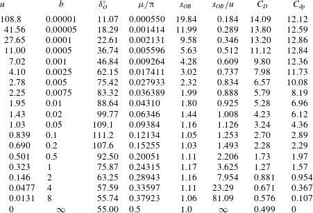
. Table 1 shows the splash jet tip angle
 $\unicode[STIX]{x1D707}$
and the ratio of the arc length of
 $s_{N_{b}-1}$
to
 $s_{OB}$
, which is the length of the splash jet between points
 $O$
and
 $B$
, for the case of
 $b=10^{-5}$
, at different
 $\unicode[STIX]{x1D6E5}=b-\unicode[STIX]{x1D702}_{N_{b}-1}=\unicode[STIX]{x1D702}_{N_{b}+1}-b$
and
 $N$
with
 $N_{b}=N/5$
. It can be seen that when
 $\unicode[STIX]{x1D6E5}=10^{-6}$
, the results have converged very well. The effects of truncations on the imaginary axis,
 $\unicode[STIX]{x1D702}_{N}$
, and on the real axis,
 $\unicode[STIX]{x1D709}_{M}$
, have also been studied, which have been found negligible when
 $\unicode[STIX]{x1D702}_{N}=\unicode[STIX]{x1D709}_{M}>10^{4}$
. In most calculations below,
 $\unicode[STIX]{x1D6E5}=10^{-6}$
,
 $N=400$
,
 $M=200$
and
 $\unicode[STIX]{x1D702}_{N}=\unicode[STIX]{x1D709}_{M}=10^{4}$
are used. It is also interesting to see from table 1 that even when
 $\unicode[STIX]{x1D6E5}=10^{-8}$
, or it is only
 $0.1\,\%$
of
 $b$
, the arc length
 $s_{N_{b}-1}$
is about
 $99\,\%$
of the total length of the splash jet
 $OB$
.
Tip angle
 $\unicode[STIX]{x1D707}/\unicode[STIX]{x03C0}$
of the splash jet and the ratio of arc length
 $s_{N_{b}-1}$
between the tip of the jet and its neighbouring node to arc length
 $OB$
.

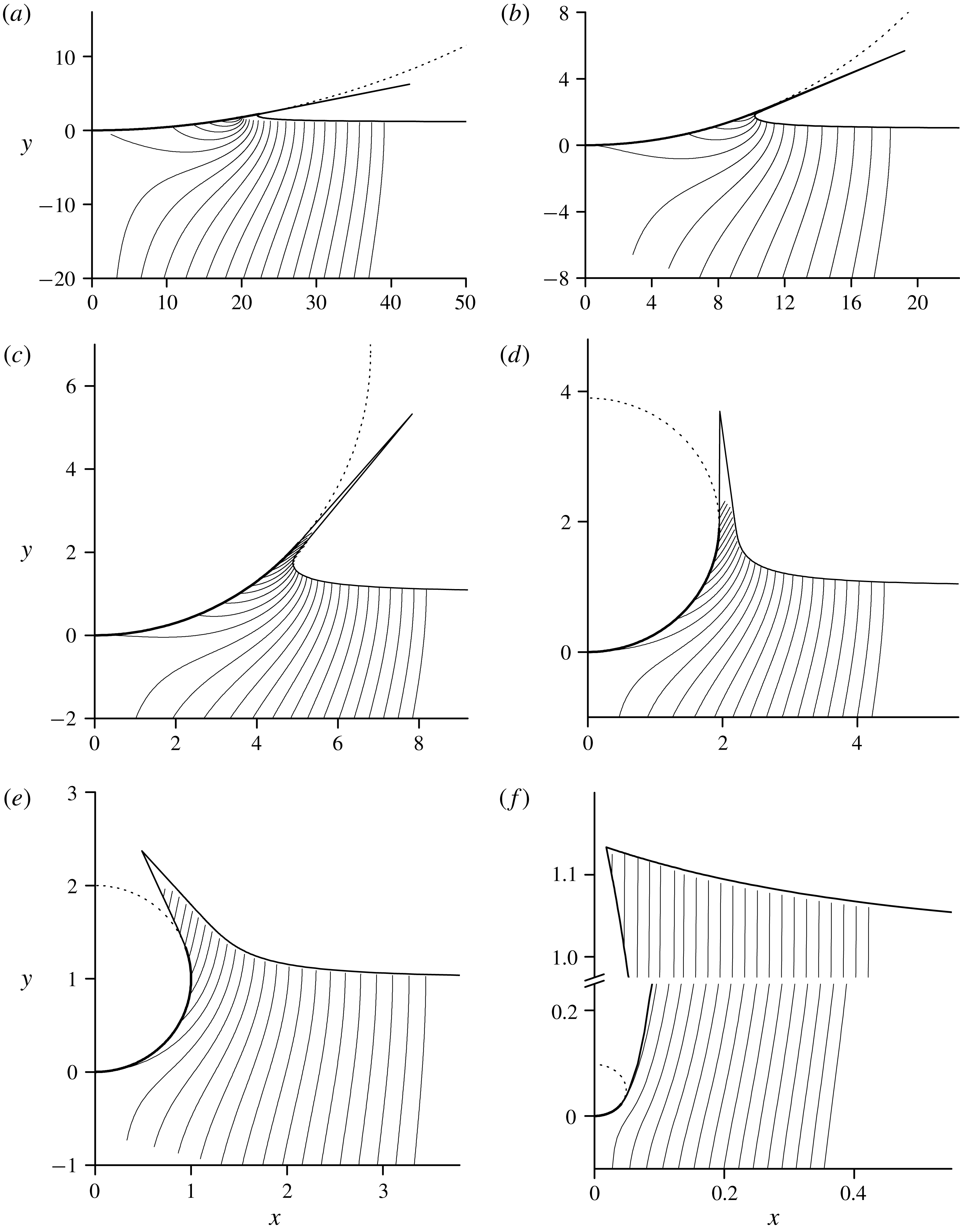
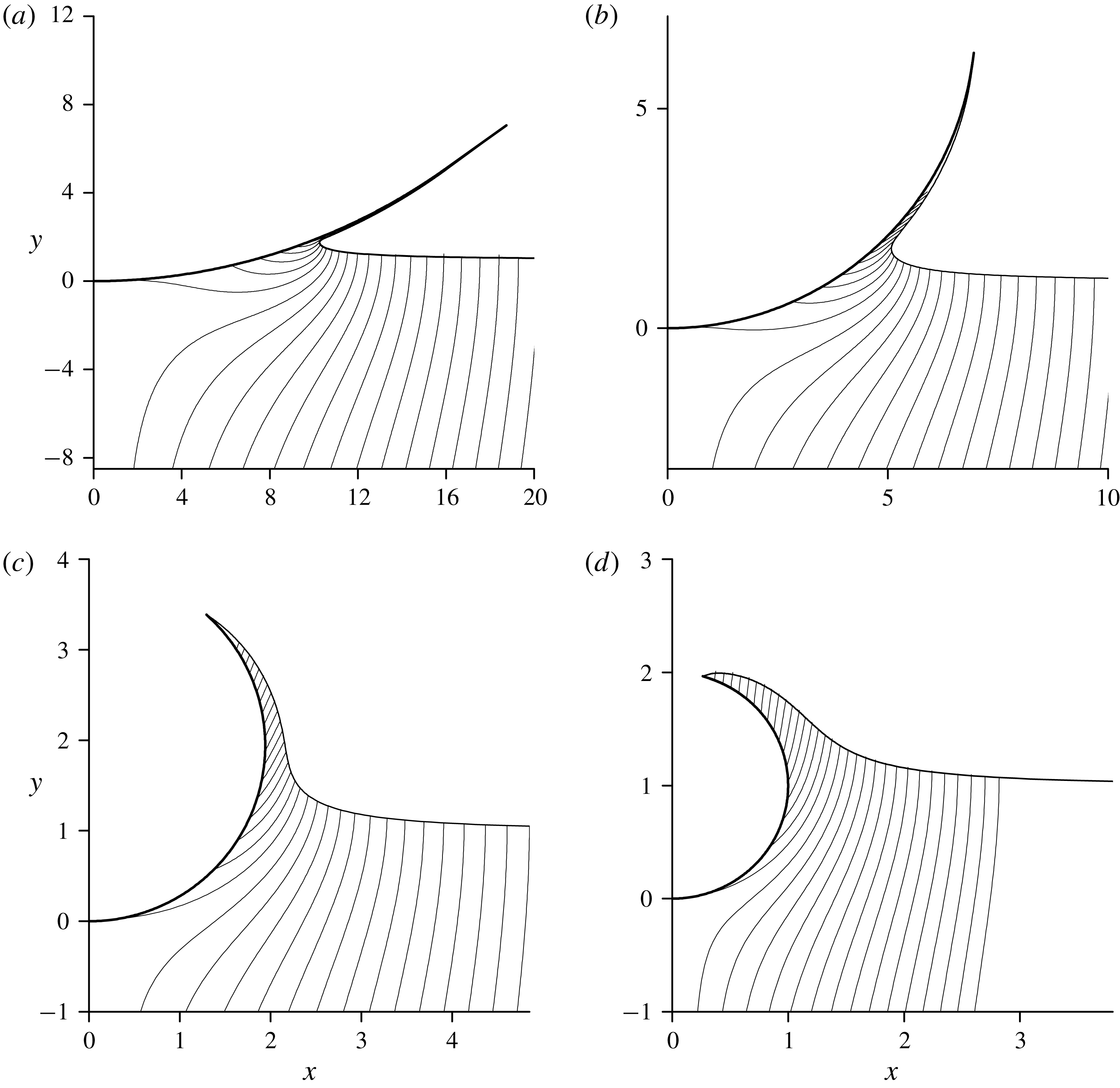
The free surface shape and streamlines for different expansion speeds of a circular cylinder: (a)
 $u=109$
,
 $b=10^{-5}$
; (b)
 $u=27.6$
,
 $b=10^{-4}$
; (c)
 $u=6.98$
,
 $b=10^{-3}$
; (d)
 $u=1.94$
,
 $b=10^{-2}$
; (e)
 $u=1.0$
,
 $b=0.052$
; (f)
 $u=0.0487$
,
 $b=4.0$
.

The streamline patterns at different expansion speeds
 $u$
, corresponding to different values of
 $b$
, are shown in figure 4. The wetted surface of the cylinder is shown by the thick line and the non-wetted surface is shown by the dashed line. The slopes of the streamlines show the flow velocity direction in the self-similar plane, and their density shows the velocity magnitude, since the flowrate between the streamlines is constant. The higher density of the streamlines occurs near the root of the splash jet. The tip angle of the splash jet is so small that lines corresponding to the two sides of the jet are very close. The zero streamline starting at the origin divides the inflow liquid coming from infinity and the liquid displaced by the volume of the cylinder and its expansion. In figure 4, it is also seen that the larger the expansion speed, the larger length of the splash jet, while its inclination to the
 $x$
-axis becomes smaller. At large expansion speeds, the length of the splash jet becomes close to the length of the wetted part of the cylinder.
The impact force coefficient
 $C_{D}$
is obtained by integration of the pressure along the wetted part of the cylinder
 $$\begin{eqnarray}\displaystyle C_{D}=\frac{2}{\unicode[STIX]{x1D70C}V^{2}R}\int _{0}^{S_{O}}(P-P_{a})\cos \unicode[STIX]{x1D6FF}_{b}\,\text{d}S_{b}=\frac{1}{u}\int _{1}^{0}c_{p}\cos \unicode[STIX]{x1D6FF}_{b}\frac{\text{d}s_{b}}{\text{d}\unicode[STIX]{x1D709}}\,\text{d}\unicode[STIX]{x1D709}. & & \displaystyle\end{eqnarray}$$
Here, the expansion speed
 $u$
, the wetted length
 $s_{O}$
of the body and the angle
 $\unicode[STIX]{x1D6FF}_{O}$
at the contact point are related through
 $u=s_{O}/\unicode[STIX]{x1D6FF}_{O}$
.
For comparison purposes, we may also compute the impact force using Wagner’s method, which is based on the approximation that the body at each stage is replaced by an equivalent horizontal plate suddenly hitting on a flat free surface. The length of the plate
 $2L$
is the horizontal distances of the two intersection points between the body surface and the free surface, and therefore, it changes with time. The force predicted by Wagner’s model for the case of the constant entry speed can be expressed as (Faltinsen Reference Faltinsen2005)
 $$\begin{eqnarray}\displaystyle F=\unicode[STIX]{x1D70C}\unicode[STIX]{x03C0}VL\frac{\text{d}L}{\text{d}t}=\unicode[STIX]{x1D70C}V^{2}RC_{dp}, & & \displaystyle\end{eqnarray}$$
where
 $C_{dp}$
is the force coefficient, similar to that in (3.5). This equation is obtained assuming that the local fluid acceleration term is much larger than that convection term in the Euler equation, or the term
 $V^{2}/2$
in the Bernoulli equation can be neglected. In the case of the expanding circular cylinder, the half length of the equivalent flat plate is chosen as
 $L=R\sin \unicode[STIX]{x1D6FF}_{O}=Vtu\sin \unicode[STIX]{x1D6FF}_{O}$
(see figure 3
a), and the angle at the flow detachment point
 $\unicode[STIX]{x1D6FF}_{O}$
is constant at a given expansion speed
 $u$
. Strictly speaking,
 $L$
here is not the same as that used in the classic Wagner theory. The contact point here is obtained from the fully nonlinear theory while in the classic Wagner theory,
 $L$
is obtained from a correction based on the solution for a flat surface. By substituting
 $L$
into (3.6), we obtain the impact force coefficient as
 $$\begin{eqnarray}\displaystyle C_{dp}=\unicode[STIX]{x03C0}u\sin \unicode[STIX]{x1D6FF}_{O}. & & \displaystyle\end{eqnarray}$$
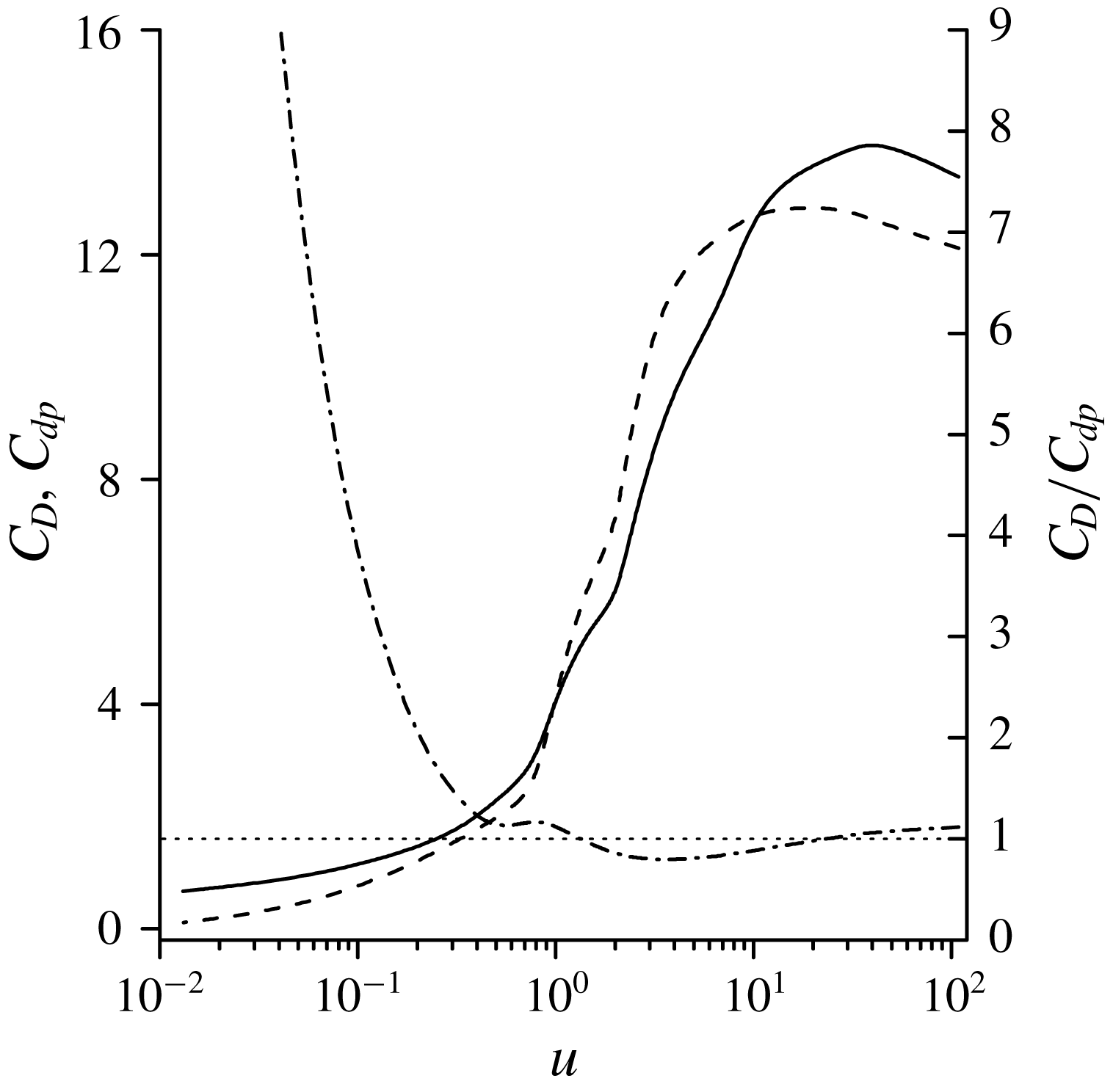
The impact force coefficient on an expanding circular cylinder entering water with constant velocity:
 $C_{D}$
in (46) (solid line);
 $C_{dp}$
in (46) (dashed line); the ratio
 $C_{D}/C_{dp}$
(dash-dotted line).

A comparison between the force coefficients predicted by (3.5) and (3.7), respectively, is shown in figure 5. As can be seen, the agreement between these models is quite good. This ratio of
 $C_{D}$
to
 $C_{dp}$
changes between
 $0.8$
and
 $1.1$
in the range of
 $0.5<u<100$
. For smaller expansion speeds,
 $C_{D}$
becomes visibly larger than
 $C_{dp}$
. This is due to the fact that the problem tends to a steady one as
 $u\rightarrow 0$
, in which the local acceleration term in the Euler equation is zero. As
 $C_{dp}$
in (3.7) is due to only local acceleration term and has ignored the convection term,
 $C_{dp}\rightarrow 0$
. Such an approximation is obviously invalid for the steady flow.
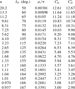
Main reference parameters for water entry of an expanding circular cylinder with detached splash jet. In the last line are shown the values corresponding to the steady flow past a circular cylinder (Gurevich Reference Gurevich1965).

The expansion velocity
 $u$
, the angle of flow detachment,
 $\unicode[STIX]{x1D6FF}_{O}^{\circ }$
, in which the superscript indicates that the angle is given in terms of degrees, the tip angle of the splash jet,
 $\unicode[STIX]{x1D707}/\unicode[STIX]{x03C0}$
, and the impact force coefficients,
 $C_{D}$
and
 $C_{dp}$
, for various values of the parameter
 $b$
are shown in table 2. It can be seen that the angle
 $\unicode[STIX]{x1D6FF}_{O}$
between the line linking body centre and its bottom
 $A$
, and the line linking its centre and the flow detachment point increases as the expansion speed decreases when it is in the range
 $0.8<u<\infty$
. The angle then starts to decrease for further decrease of the expansion speed in the range
 $0<u<0.8$
. For the very small expansion speed, the angle approaches the value
 $\unicode[STIX]{x1D6FF}_{O}\approx 55^{\circ }$
, which is the angle at the flow detachment point for the steady flow past a fixed circular cylinder (Gurevich Reference Gurevich1965). In this case, the length of the free surface
 $OB$
tends to infinity and becomes one side of an open cavity. It is known that the half width of the steady cavity,
 $X_{c}$
, tends to infinity at a rate of
 $X_{c}\sim \ln Y_{c}$
(Gurevich Reference Gurevich1965). However, in the similarity plane, the coordinate
 $x_{c}=X_{c}/(Vt)\sim \ln (Vt)/(Vt)\rightarrow 0$
as can be seen in figure 4(f).
The results in table 2 show that for
 $b\rightarrow 0$
the angle of the splash jet,
 $\unicode[STIX]{x1D707}$
, tends to zero. For this reason, the length
 $s_{OB}$
does not tend to zero. In fact, when
 $b\rightarrow 0$
, (3.3a
) gives
 $s_{OB}$
if
 $\unicode[STIX]{x1D702}_{Nb-1}$
is taken as
 $0$
. Thus
 $$\begin{eqnarray}\displaystyle s_{OB}=\frac{\unicode[STIX]{x03C0}K_{b}}{\unicode[STIX]{x1D707}}b^{2\unicode[STIX]{x1D707}/\unicode[STIX]{x03C0}}. & & \displaystyle\end{eqnarray}$$
Therefore, it seems that the result for
 $b\rightarrow 0$
is different from that for
 $b=0$
. However, in reality, when
 $\unicode[STIX]{x1D707}\rightarrow 0$
and if the jet thickness tends to zero, the existence of such a jet does not affect the main flow, as the integrations along the both sides of the jet virtually cancel each other. Thus, removal of such a jet would not be expected to make a real difference to the solution. In such a case, the flow is virtually the same as the attached flow, where
 $O$
is the contact point or the root of the attached jet, which will be discussed further later. It should also be noted that although
 $s_{OB}$
increases as
 $b$
decreases in table 2,
 $s_{OB}/u$
decreases. In other words, relative to the size of the cylinder, the effect of
 $s_{OB}$
on the global flow decreases as
 $b\rightarrow 0$
.
3.2 An expanding circular cylinder with attached flow
The computation for an expanding cylinder with attached flow is also a challenging task, especially at small
 $\unicode[STIX]{x1D707}$
as the singularity of order
 $2\unicode[STIX]{x1D707}/\unicode[STIX]{x03C0}-1$
in (2.46) tends to
 $\unicode[STIX]{x1D701}^{-1}$
as
 $\unicode[STIX]{x1D707}\rightarrow 0$
. Although the nodes
 $\unicode[STIX]{x1D702}_{j}$
and
 $\unicode[STIX]{x1D709}_{j}$
are distributed as a geometric series, it is found that even when
 $\unicode[STIX]{x1D702}_{1}=\unicode[STIX]{x1D709}_{1}=10^{-6}$
are used next to the origin
 $\unicode[STIX]{x1D701}=0$
the arc length
 $s_{\unicode[STIX]{x1D702}_{1}}$
and
 $s_{\unicode[STIX]{x1D709}_{1}}$
from the nearest nodes to the intersection point
 $O$
, on the free surface and the body surface, respectively, are still not sufficiently small. As shown in table 1 for the detached flow, the arc length from the nearest node to the tip of the jet is about
 $99\,\%$
of the total length of the jet. Such a large percentage arc length taken by a single element does not cause a major problem for the case of the detached flow, because boundaries of the jet are nearly straight lines and the velocity field in the jet is almost uniform in the same direction. However, for the jet attached on a curved surface, the length of the element
 $S_{\unicode[STIX]{x1D709}_{1}}$
should be small enough to account for the shape of the cylinder and its effect on the flow in the jet. This difficulty can be resolved by introducing the following variables:
 $$\begin{eqnarray}\displaystyle \ln \unicode[STIX]{x1D701}=\ln |\unicode[STIX]{x1D701}|+\arg \unicode[STIX]{x1D701}=\left\{\begin{array}{@{}ll@{}}\unicode[STIX]{x1D711}_{\unicode[STIX]{x1D709}}, & \unicode[STIX]{x1D701}=\unicode[STIX]{x1D709},\\ \unicode[STIX]{x1D711}_{\unicode[STIX]{x1D702}}+\text{i}\unicode[STIX]{x03C0}/2, & \unicode[STIX]{x1D701}=\text{i}\unicode[STIX]{x1D702},\end{array}\right. & & \displaystyle\end{eqnarray}$$
where the subscript refers to the axis on which the corresponding variable is defined. We then rewrite the system of integro-differential equations (2.17), (2.20), (2.27) and (2.28) based on variables
 $\unicode[STIX]{x1D711}_{\unicode[STIX]{x1D709}}$
and
 $\unicode[STIX]{x1D711}_{\unicode[STIX]{x1D702}}$
. It can be seen that using
 $$\begin{eqnarray}\displaystyle \frac{\text{d}}{\text{d}\unicode[STIX]{x1D711}_{\unicode[STIX]{x1D709}}}-\left(\unicode[STIX]{x1D701}\frac{\text{d}}{\text{d}\unicode[STIX]{x1D701}}\right)_{\unicode[STIX]{x1D701}=\unicode[STIX]{x1D709}} & & \displaystyle\end{eqnarray}$$
the singularity at
 $\unicode[STIX]{x1D701}=0$
in (2.46) and (2.47) disappears, and we can determine the arc length coordinate along the free surface,
 $s(\unicode[STIX]{x1D711}_{\unicode[STIX]{x1D702}})$
, and along the body,
 $s(\unicode[STIX]{x1D711}_{\unicode[STIX]{x1D709}})$
, as follows:
 $$\begin{eqnarray}\displaystyle s(\unicode[STIX]{x1D711}_{\unicode[STIX]{x1D702}})=-\int _{-\infty }^{\unicode[STIX]{x1D711}_{\unicode[STIX]{x1D702}}}\frac{1}{v(\unicode[STIX]{x1D711}_{\unicode[STIX]{x1D702}})}\left|\frac{\text{d}w}{\text{d}\unicode[STIX]{x1D711}_{\unicode[STIX]{x1D702}}}\right|\text{d}\unicode[STIX]{x1D711}_{\unicode[STIX]{x1D702}},\quad s(\unicode[STIX]{x1D711}_{\unicode[STIX]{x1D709}})=\int _{-\infty }^{\unicode[STIX]{x1D711}_{\unicode[STIX]{x1D709}}}\frac{1}{v(\unicode[STIX]{x1D711}_{\unicode[STIX]{x1D709}})}\left|\frac{\text{d}w}{\text{d}\unicode[STIX]{x1D711}_{\unicode[STIX]{x1D709}}}\right|\text{d}\unicode[STIX]{x1D711}_{\unicode[STIX]{x1D709}} & & \displaystyle\end{eqnarray}$$
similar to the way of determining
 $s(\unicode[STIX]{x1D702})$
and
 $s_{b}(\unicode[STIX]{x1D709})$
in (2.18) and (2.26), respectively. Then equation (3.3) for the arc lengths of the nodes nearest to the tip takes the form
 $$\begin{eqnarray}\displaystyle \{s_{\unicode[STIX]{x1D709}_{1}},-s_{\unicode[STIX]{x1D702}_{1}}\}=\frac{\unicode[STIX]{x03C0}K}{2\unicode[STIX]{x1D707}v_{0}}\exp \left[-\frac{1}{\unicode[STIX]{x03C0}}\int _{0}^{\infty }\frac{\text{d}\unicode[STIX]{x1D6FE}}{\text{d}\unicode[STIX]{x1D711}_{\unicode[STIX]{x1D709}}}\unicode[STIX]{x1D711}_{\unicode[STIX]{x1D709}}\,\text{d}\unicode[STIX]{x1D711}_{\unicode[STIX]{x1D709}}+\frac{1}{\unicode[STIX]{x03C0}}\int _{0}^{\infty }\frac{\text{d}\unicode[STIX]{x1D706}}{\text{d}\unicode[STIX]{x1D711}_{\unicode[STIX]{x1D702}}}\unicode[STIX]{x1D711}_{\unicode[STIX]{x1D702}}\,\text{d}\unicode[STIX]{x1D711}_{\unicode[STIX]{x1D702}}+\frac{2\unicode[STIX]{x1D707}}{\unicode[STIX]{x03C0}}\{\unicode[STIX]{x1D711}_{\unicode[STIX]{x1D709}},\unicode[STIX]{x1D711}_{\unicode[STIX]{x1D702}}\}\right]. & & \displaystyle \nonumber\\ \displaystyle & & \displaystyle\end{eqnarray}$$
In the discrete form, the solution is sought on two sets of points,
 $\unicode[STIX]{x1D711}_{min}<\unicode[STIX]{x1D711}_{\unicode[STIX]{x1D709}_{j}}<\unicode[STIX]{x1D711}_{max}$
,
 $j=1,\ldots ,M$
and
 $\unicode[STIX]{x1D711}_{min}<\unicode[STIX]{x1D711}_{\unicode[STIX]{x1D702}_{j}}<\unicode[STIX]{x1D711}_{max}$
,
 $j=1,\ldots ,N$
, corresponding to the real and imaginary axes. Based on the computational studies, the range of the interval,
 $\unicode[STIX]{x1D711}_{min}=-200$
and
 $\unicode[STIX]{x1D711}_{max}=30$
is chosen to capture the flow details near the tip of the jet. These values correspond to
 $\unicode[STIX]{x1D702}_{min}=10^{-87}$
and
 $\unicode[STIX]{x1D702}_{max}=10^{4}$
in the
 $\unicode[STIX]{x1D701}$
-plane. The total number of points is chosen with
 $N=600$
and
 $M=600$
based on the study of convergence and the accuracy of the solution procedure.
The flow configuration at the different expansion speeds: (a)
 $u=27.6$
; (b)
 $u=6.98$
; (c)
 $u=1.94$
; (d)
 $u=1.0$
.

The streamline patterns for the different expansion speeds together with the free surface shape are shown in figure 6. It can be seen within the range calculated that the larger the expansion speed is, the smaller angle
 $\unicode[STIX]{x1D6FF}_{O}$
and the thinner the jet will be, which is similar to those observed in figure 4 for the detached flow configuration. However, in contrast to the detached flow, for which a solution can be obtained in the whole range of expansion speeds, from zero to infinity, for the attached flow there is a minimal expansion speed, or maximal angle
 $\unicode[STIX]{x1D6FF}_{O}$
, for which the solution with a free surface can be obtained. For expansion speeds smaller than that no converged solution can be obtained from the numerical procedure.
Relative to the bottom of the body
 $A$
, the top of the body moves in the
 $y$
direction with speed
 $2u$
. Noticing the velocity of the incoming flow is
 $1$
, if
 $1>2u$
, or
 $u<0.5$
, the top of the cylinder will be below the undisturbed free surface. In such a case, the cylinder becomes fully enclosed by the liquid, and the solution with a contact point
 $O$
between the body surface and the free surface no longer exists. Due to the attached jet, its tip
 $O$
may reach the top of the cylinder and the cylinder becomes fully enclosed by the liquid at
 $u$
larger than
 $0.5$
. In such a case, a solution for a contact point
 $O$
is possible only for the detached flow.
(a) The free surface shapes and the streamlines near the jet tip at the different angles of the wetted part of the cylinder
 $\unicode[STIX]{x1D6FF}_{O}$
, and (b) free surface shape and velocity magnitude along the free surface at
 $\unicode[STIX]{x1D6FF}_{O}=167^{\circ }$
for
 $u=0.9365$
.

The streamlines inside jets attached on the body at
 $u=1.069,1.005,0.937$
with the corresponding angles
 $\unicode[STIX]{x1D6FF}_{O}=163^{\circ },165^{\circ }$
and
 $\unicode[STIX]{x1D6FF}_{O}=167^{\circ }$
, the last of which is the largest angle that could be obtained computationally, are shown in figure 7(a). It is seen that the angle between the streamlines and the cylinder surface increases for larger angle
 $\unicode[STIX]{x1D6FF}_{O}$
and the streamlines become almost perpendicular to the cylinder near the tip of the jet as is seen in figure 7(a). Therefore, the tangential component velocity on the cylinder surface gradually decreases along the body surface toward to the tip.
The velocity magnitude distribution along the free surface is shown in figure 7(b) for
 $\unicode[STIX]{x1D6FF}_{O}=167^{\circ }$
that corresponds to the expansion speed
 $u=0.8365$
. It is seen that there is a maximum of the magnitude, whose position is around the point of inflection of the free surface. The magnitude of the velocity decreases towards the contact point. Such a behaviour of the velocity is different from that observed for wedges entering the liquid, for which the velocity along the free surface reaches its maximal value at the jet tip (Dobrovol’skaya Reference Dobrovol’skaya1969; Zhao & Faltinsen Reference Zhao and Faltinsen1993).
(a) Velocity magnitude along the free surface relative to the velocity at the jet tip,
 $v/v_{0}$
, (lower set of the curves) and the angle of the velocity to the free surface,
 $\unicode[STIX]{x1D703}$
, (upper set of the curves) for different expansion speeds:
 $u=20.2$
,
 $\unicode[STIX]{x1D6FF}_{O}=50^{\circ }$
(dashed-dot lines);
 $u=5.62$
,
 $\unicode[STIX]{x1D6FF}_{O}=90^{\circ }$
(dotted line);
 $u=2.09$
,
 $\unicode[STIX]{x1D6FF}_{O}=135^{\circ }$
(dashed line);
 $u=0.937$
,
 $\unicode[STIX]{x1D6FF}_{O}=167^{\circ }$
(solid line).

The velocity magnitude along the free surface relative to that at the tip of the jet, and the angle of the velocity to the free surface against
 $s/v_{0}$
are shown in figure 8 for the different expansion speeds. It is clearly seen that the maximum of the velocity magnitude occurs at
 $s/v_{0}$
from
 $0.5$
to
 $0.6$
, and within this range, both sets of results change rapidly apart from that at the critical case of
 $u=0.937$
. Rapid variation near the jet root is a typical behaviour of the velocity in water entry of blunt bodies/wedges (Howison et al.
Reference Howison, Ockendon and Wilson1991; Zhao & Faltinsen Reference Zhao and Faltinsen1993). Along the jet towards its tip, the velocity magnitude decreases while the angle of the velocity to the free surface slightly increases. This is due to the effect of the curvature of the body surface along which the jet is running.


The pressure coefficient on the cylinder surface is shown in figure 9 for different expansion speeds. Results from detached flow at the same expanding speed are also provided. It is seen that for both attached and detached flow configurations, the pressure distributions along the cylinder are almost the same in the wide range of expansion speeds, including the pressure peaks near the jet root. This means that the pressure distribution on the body is not very much affected by the flow detachment. A small difference between pressures in the detached and attached flows occurs beyond the jet root. In the former, the pressure drops rapidly to zero at the detachment point
 $O$
(
 $x_{O},y_{O}$
). In the latter case, the pressure will also drop rapidly from the jet root near point (
 $x_{O},y_{O}$
). However, because the flow is attached on the body beyond this point, the pressure on the body surface is not the ambient one. In fact, it will keep decreasing and become smaller than the ambient pressure, leading to a negative
 $c_{p}$
. The pressure coefficient in the attached flow returns to zero at its own contact point. For the lower expansion speeds shown in figure 9(c,d), the corresponding jets become thicker, as can be seen in figure 6. However, the magnitude of the negative pressure coefficients become smaller than those for larger expansion speeds in figure 9(a,b).
Main reference parameters for water entry of an expanding circular cylinder with attached flow.

The main flow characteristics for different expansion speeds are shown in table 3. The angle at the contact point and the angle at the jet tip both monotonically increase as the expansion speed decreases. At the lowest possible expansion speed
 $u=0.937$
for the attached flow they become
 $\unicode[STIX]{x1D6FF}_{O}=167^{\circ }$
and
 $\unicode[STIX]{x1D707}=61^{\circ }$
, respectively. In table 3, the force coefficients for the attached (
 $C_{D}^{\prime }$
) and detached (
 $C_{D}^{\prime \prime }$
) flows are also shown. As expected from the previous discussion, for the same expansion speed of the cylinder they are very close to each other.
We may relate what has been found in the present study on an expanding body to that on a body of fixed size entering water. For the latter, in the case of a circular cylinder, its radius
 $R=R_{0}$
will be a constant. Based on the present notation,
 $u=R_{0}/(Vt)$
will then change with time. The problem of a cylinder with constant
 $R_{0}$
is obviously fully transient. The problem was considered by Greenhow (Reference Greenhow1988) who adopted the numerical method of Vinje & Brevig (Reference Vinje and Brevig1981). The calculations started from a moment at which the body already had some finite depth of penetration into the liquid. Here, we may assume that at each given time, the self-similar solution can still shed some light. In fact, this practice has been used by Semenov & Wu (Reference Semenov and Wu2016) for an expanding wedge and expanding plate, and close correlation between the results of the transient flow and self-similar flow has been found. Here, at early stage of water entry of a fixed cylinder,
 $u$
is very large. Although both detached flow and the attached flow are possible, the thickness of the detached jet in the former and that of the attached jet in the latter are both extremely small. The jets in both cases hardly affect the main physical parameters, such as the pressure distribution on the body surface. In other words, when jets are removed, both flows can be treated as attached with the intersection point near the jet root. When
 $t$
increases,
 $u$
will decrease. Although the jets in both flows are no longer very thin, the above practice at small
 $t$
or large
 $u$
still works very well and the pressure distributions on the body surface up to the jet root are nearly the same. This suggests that no matter whether the detached flow or attached model is used, the pressure distribution is not very different. As
 $t$
further increases, the detached flow will eventually tend to the steady Helmholtz flow. For the attached flow, the solution with an intersection point between the free surface and the body surface is no longer possible, as the body will be fully enclosed by the fluid. Thus, the present self-similar solutions for detached and attached flows closely reflect what has been observed by Duez et al. (Reference Duez, Ybert, Clanet and Bocquet2007) for hydrophobic and hydrophilic bodies, respectively.
4 Conclusions
Self-similar solutions for water entry of an arbitrarily shaped body in expansion have been obtained based on the velocity potential theory, with gravity and surface tension effects being ignored. Both cases with flow detached from a hydrophobic body and flow attached on a hydrophilic body have been considered. The integral hodograph method has been employed in the parameter plane in which the derivative of the complex potential is expressed together with the complex velocity. Through the method, the original problem in the whole fluid domain was reduced to a system of integral and integro-differential equations in which the dynamic and kinematic boundary conditions on the free surface and the impermeable condition on the body surface are imposed.
For the detached flow, the condition of velocity continuity and the boundedness of the spatial derivative of the velocity was imposed at the point of the detachment, which was used to locate the position of the detachment point. It was then found that the curvature of the free surface is equal to that of the body surface at the detachment point in this self-similar flow, which means that the Brillouin–Villat condition for the steady flow also holds in the present problem.
The solution of the problem very much depends on the ratio of the expansion speed to the entry speed
 $u$
. At large
 $u$
, which corresponds to the early stage of a fixed cylinder or small
 $t$
, both detached and attached flows are mathematically possible. However, the main results, such as pressure distributions on the body up to the point near the jet root are nearly the same, suggesting that either model could be used. As
 $u$
decreases, or the corresponding
 $t$
increases for a fixed cylinder, the thicknesses of the jets in the two flows are no longer small. Their shapes are quite different. However, the pressure distributions on the body surface in both cases are still very close to each other. A difference is that in the attached flow, the pressure in the jet region becomes smaller than the ambient pressure. As
 $u$
further decreases, or
 $t$
further increases for a fixed cylinder, the solution for the detached flow can still be found. As
 $u\rightarrow 0$
, the solution approaches the steady free-streamline Helmholtz flow past the curved body with an infinitely long cavity. For the attached flow, there is a minimal value of
 $u$
, below which no solution can be found. It has been found through numerical computation that the minimal value is
 $u\approx 0.93$
for a circular cylinder. For a fixed cylinder, very small
 $u$
corresponds to very large
 $t$
. In such a case, the body will be fully enclosed by the fluid. The attached flow with a contact point between the body surface and the free surface is no longer possible and the attached flow means that the whole body surface becomes the wetted surface.
It has also been found that the Wagner theory gives good results when
 $u>0.5$
for the expanding circular cylinder. For smaller
 $u$
, the results from the Wagner theory become inaccurate. This reflects the fact that in the Wagner theory, the velocity product term is ignored and only the temporal derivative is kept in the Bernoulli equation, based on the assumption that the former is much smaller than the latter. Such an assumption becomes invalid at small
 $u$
, as the problem tends to steady and the temporal derivative tends to zero.
Acknowledgements
This work is supported by Lloyd’s Register Foundation (LRF) through the joint centre involving University College London, Shanghai Jiaotong University and Harbin Engineering University, to which the authors are most grateful. LRF supports the advancement of engineering-related education, and funds research and development that enhances the safety of life at sea, on land and in the air.