2.1. Hypotheses of Interest

Suppose g(I_t−1,θ) is a parametric model for the conditional mean E(Y_t|I_t−1) of a stochastic time series process {Y_t}, where I_t−1 is an information set at time t − 1, which may contain lagged dependent variables {Y_t−j,j > 0} and current and lagged exogenous variables {Z_t−j,j ≥ 0}, and θ ∈ Θ is a finite-dimensional parameter. Examples of g(I_t−1,θ) include linear time series regression (static or dynamic) models, autoregressive moving average (ARMA) models, ARMA with exogenous variables (ARMAX) models, regime-switching autoregressive models (Hamilton, 1989), parametric state-space models (Priestley, 1988), smooth transition autoregressive models (Teräsvirta, 1994), Poisson jump autoregressive models, and threshold autoregressive models with known thresholds (e.g., Potter, 1995).¹

We say that the model g(I_t−1,θ) is correctly specified for E(Y_t|I_t−1) if

Alternatively, the model g(I_t−1,θ) is misspecified for E(Y_t|I_t−1) if

Conditional mean modeling has been a primary interest in time series analysis, because E(Y_t|I_t−1) is the optimal predictor for Y_t using I_t−1 in terms of the mean squared error criterion. In addition, most dynamic economic theories have implications on and only on the conditional mean dynamics of economic processes, as pointed out earlier.

2.2. Generalized Spectral Derivative Tests

In time series modeling, I_t−1 is possibly infinite-dimensional (i.e., dating back to the infinite past), as is the case for non-Markovian processes. This poses a challenge in testing the adequacy of the model g(I_t−1,θ), due to the curse of dimensionality. Hong and Lee (2005) proposed a nonparametric test of

using a suitable partial derivative of the Hong (1999) generalized spectrum, which avoids the curse of dimensionality. Define the model error

Then

holds if and only if E [ε_t(θ₀)|I_t−1] = 0 a.s. for some θ₀ ∈ Θ. The null hypothesis

thus implies E [ε_t(θ₀)|I_t−1^ε] = 0 a.s., where I_t−1^ε ≡ {ε_t−1(θ₀),ε_t−2(θ₀),…}. This forms a basis for testing

.

For notational economy, we put ε_t ≡ ε_t(θ₀), where

and

is a parameter estimator. Suppose {ε_t} is a strictly stationary process with marginal characteristic function φ(u) ≡ E(e^iuε_t) and pairwise joint characteristic function φ_j(u,v) ≡ E(e^{iuε_t+ivε_{t−| j|}}), where

,

, and j = 0,±1,… The basic idea of the generalized spectrum in Hong (1999) is to consider the spectrum of the transformed series {e^iuε_t}. It is defined as

where ω is the frequency and σ_j(u,v) ≡ cov(e^iuε_t,e^{ivε_{t−| j|}}) is the covariance function of the transformed series. The function f (ω,u,v) can capture any type of pairwise serial dependence in {ε_t}, i.e., dependence between ε_t and ε_t−j for any j ≠ 0, including nonlinear serial dependence with zero autocorrelation. This is analogous to the higher order spectra (Brillinger, 1965; Brillinger and Rosenblatt, 1967a, 1967b). Unlike the higher order spectra, however, f (ω,u,v) does not require the existence of any moment of {ε_t}. Nevertheless, when E(ε_t²) exists, we can obtain the power spectrum as a partial derivative of f (ω,u,v) at (u,v) = (0,0):

For this reason, we call f (ω,u,v) the generalized spectrum of {ε_t}.

As is well known, the interpretation of spectral analysis is more difficult for nonlinear time series than for linear time series. For example, the bispectrum (e.g., Subba Rao and Gabr, 1984) has no physical (i.e., energy decomposition over frequencies) interpretation, unlike the power spectrum. This is also true of f (ω,u,v). However, the basic idea of characterizing cyclical dynamics still applies: f (ω,u,v) is useful when searching for linear or nonlinear cyclical movements. A strong cyclicity of data can be linked with a strong serial dependence in {ε_t} that may not be captured by the autocorrelation function. The generalized spectrum f (ω,u,v) can capture such nonlinear cyclical patterns by displaying distinct spectral peaks. This can be seen from the Taylor series expansion of f (ω,·,·) around the origin (0,0):

assuming all moments of {ε_t} exist. Now suppose an asset series is a white noise (cov(ε_t,ε_t−j) = 0 for all j ≠ 0) but has a stochastic cyclical dynamics in volatility clustering, which may be linked to business cycles (e.g., Schwert, 1989; Hamilton and Lin, 1996). Then the power spectrum will miss these volatility cycles, but f (ω,u,v) can effectively capture them. More generally, f (ω,u,v) can capture cyclical dynamics in the conditional distribution of {ε_t}, including those in volatility, skewness, and kurtosis.²

The generalized spectrum f (ω,u,v) itself is not suitable for testing

, because it can capture serial dependence not only in mean but also in higher order moments.

The generalized spectrum f (ω,u,v) is suitable for testing the i.i.d. hypothesis for {ε_t} as is considered in Hong and Lee (2003). It is not suitable for testing

, because {ε_t} can be an m.d.s. but not an i.i.d. sequence.

where

The measure σ_j⁽¹⁰⁾(0,v) checks whether the autoregression function E(ε_t|ε_t−j) at lag j is zero. Under appropriate regularity conditions, σ_j⁽¹⁰⁾(0,v) = 0 for all

if and only if E(ε_t|ε_t−j) = 0 a.s.

The use of E(ε_t|ε_t−j) or σ_j^(1,0)(0,v) for testing

is analogous in spirit to the nonparametric additive models in the nonparametric estimation literature (e.g., Kim and Linton, 2004).

Although E(ε_t|ε_t−j) and σ_j⁽¹⁰⁾(0,v) are equivalent measures, the use of σ_j⁽¹⁰⁾(0,v) avoids smoothed nonparametric estimation. Moreover,

can be viewed as an operational measure of the maximum mean correlation, max_{f (·)}|corr[ε_t,f (ε_t−j)]|, which was proposed by Granger and Teräsvirta (1993, p. 23) as a measure for nonlinearity in mean. Similarly, the generalized spectral derivative modulus

can be viewed as the maximum dependence in mean at frequency ω. It can be used to search cycles in mean that are caused by linear or nonlinear serial dependence in mean (e.g., ARCH-in-mean effect; see Engle, Lilien, and Robins, 1987).⁶

Because ε_t is not observed, we need to use an estimated model residual

where I_t−1^[dagger] is the information set observed at time t − 1 that may involve some assumed initial values.

For example, consider an MA(1) model:

. Here, the infeasible information set I_t−1 = {Y_t−1,Y_t−2,…,Y₁,Y₀,…} contains the entire past history {Y_s,s < t} dating back to the infinite past. On the other hand, I_t−1^[dagger] = {Y_t−1,Y_t−2,…,Y₁,ε₀}, where ε₀ is an assumed initial value for ε₀.

-consistent parameter estimator

can be used. Examples of

are the conditional least squares and quasi–maximum likelihood estimators. With

, one can consistently estimate f⁽⁰¹⁰⁾(ω,0,v) by a smoothed kernel estimator

where

, and

. Here, p ≡ p(T) is a bandwidth, and

is a symmetric kernel. Examples of k(·) include the Bartlett, Daniell, Parzen, and quadratic spectral kernels (e.g., Priestley, 1981, p. 442). The factor (1 − | j|/T)^1/2 is a finite-sample correction. It could be replaced by unity.

Under

, the generalized spectral derivative f⁽⁰¹⁰⁾(ω,0,v) is a “flat” spectrum:

which can be consistently estimated by

To test

, Hong and Lee (2005) compared

and

via an L₂-norm. Their test statistic is

where

is a nondecreasing function that weighs sets symmetric about zero equally,

Throughout, all unspecified integrals are taken on the support of W(·). An example of W(·) is the N(1,0) cumulative distribution function (c.d.f.), which is commonly used in the characteristic function literature. The factors

and

are the approximate mean and variance of the quadratic form

. They have taken into account the impact of conditional heteroskedasticity and time-varying higher order conditional moments. As a result,

is robust to conditional heteroskedasticity and time-varying higher order conditional moments of unknown form.

Hong and Lee (2005) also considered two other classes of generalized spectral tests, derived under conditional homoskedasticity and i.i.d. regression errors, respectively. These tests can also be modified in the same way as we do for

to remove the impact of parameter estimation uncertainty.

and

grow to infinity at a rate of p as p → ∞, p/T → 0.

Hong and Lee (2005) showed that

under

. Because the parametric estimator

converges to θ₀ faster than the rate at which the nonparametric kernel estimator

converges to f⁽⁰¹⁰⁾(ω,0,v), the asymptotic normal distribution of

is solely determined by

. Attractively,

can be any

-consistent estimator of θ₀, and parameter estimation uncertainty has no impact on the asymptotic distribution of

. In other words, the asymptotic distribution of

is unchanged when

is replaced by its probability limit θ₀. This results in significant simplification of some otherwise difficult contexts. In particular, only estimated model residuals are needed to compute the test statistics.

However, the convenient asymptotic nuisance parameter–free property is not without cost for

. Although parameter estimation uncertainty has no impact on the asymptotic distribution of

, it has an impact on the finite-sample distribution. Because g(I_t−1,θ) is a parametric model,

can result in at most an adjustment of a finite number of degrees of freedom to the distribution of

. When the lag order p → ∞ as T → ∞, the impact of

becomes negligible when normalized by the standard deviation estimator

, which grows to infinity at the rate of p^1/2. However, asymptotic analysis reveals that the asymptotically negligible higher order terms in

that are associated with parameter estimation uncertainty vanish to zero in probability rather slowly, as will be seen subsequently. Therefore,

may significantly distort the size of

in small and finite samples. This is particularly the case when there are relatively many parameters but the sample size T is not large, as is typically encountered for macroeconomic time series data and low-frequency financial time series data.

2.3. Wooldridge's Device

In a series of important works, Wooldridge (1990a, 1990b, 1991) proposed a unified approach to robust, regression-based parametric specification tests for possibly dynamic time series models, including time series conditional mean models. Wooldridge (1990a) considered the null hypothesis

where φ_t(θ) is a measurable, possibly vector-valued function. In the present context, φ_t(θ) = iε_t(θ) in (2.1). Wooldridge (1990a) used a test function Λ_t(θ) ∈ I_t−1 and checked if E [Λ_t(θ₀)φ_t(θ₀)] = 0 by using the sample moment

where

,

, and

is a

-consistent estimator of θ₀. Straightforward algebra shows that

where Φ_t(θ₀) ≡ E [(∂/∂θ)φ_t(θ₀)|I_t−1]. Thus, the asymptotic distribution of

is jointly determined by

and

, unless Φ_t(θ₀) = 0 under the null hypothesis.

To remove the impact of parameter estimation uncertainty of

on the asymptotic distribution of

, Wooldridge (1990a) first purged from

its linear projection onto

, a consistent estimator for Φ_t(θ₀), and then considered the modified test statistic

where

is the ordinary least squares (OLS) estimator of regressing

on

. It can be shown that for any

-consistent estimator

,

where

. Thus, the asymptotic distribution of

is robust to parameter estimation uncertainty because it is not affected by any

-consistent estimator

up to O_P(T^−1/2). An asymptotic χ² test can be obtained by forming a suitable quadratic form in

. We note that the Wooldridge (1990a) device does not imply that

has a better asymptotic approximation than

in finite samples or vice versa. However, it nicely generates a new set of moment conditions

that is robust to parameter estimation uncertainty up to O_P(T^−1/2). Consequently, its asymptotic distribution does not depend on any

-consistent estimator

. This makes the test based on

rather convenient in practice.

Although the Wooldridge (1990a) device may not deliver a better asymptotic distribution approximation for

, it ideally suits our purpose of improving the finite-sample performance of the generalized spectral derivative test

in (2.6), because with a new set of moment conditions, it can make the asymptotically negligible higher order terms in

that are associated with

vanish faster to 0. Subsequently, we first describe how the Wooldridge (1990a) device can be adapted to

and then explain why it can improve the asymptotic normal approximation for

.

Although

is more complicated than the Wooldridge (1990a) test statistic, the Wooldridge (1990a) device can be applied to each generalized covariance derivative

, which has a similar structure to

, with

and

. Based on this observation, we introduce a modified generalized covariance

where

,

, and

The modified generalized spectral derivative estimators can then be defined as follows:

and

Comparing

and

via an L₂-norm, we obtain the modified test statistic

where the centering and scaling factors

To gain insight into why the Wooldridge (1990a) device can improve the finite-sample performance of

, we now provide heuristics. Put ψ_t(v) = e^ivε_t − φ(v), G_t = (∂/∂θ)g(I_t−1,θ₀), ξ_t−j(v) = ivG_t−j e^ivε_t−j, and η_j(v) = E [G_tψ_t−j(v)] for j > 0 and let

be defined in the same way as

with {ε_t}_t=1^T replacing

. Then, by a Taylor series expansion around θ₀, we have for each j > 0,

where the remainder O_P [(T − j)⁻¹] term in the first equality comes from the higher order terms of the Taylor series expansion, including the effect of replacing the information set I_t−1^[dagger] with I_t−1. The last equality follows from

, Chebyshev's inequality,

under the m.d.s. property of {ε_t} as implied by

, and

under suitable mixing conditions on the time series process {ε_t,G_t′}′.

For static conditional mean models where g(I_t−1,θ₀) is only a function of strictly exogenous variables independent of innovations {ε_t}, we have η_j(v) = 0 for all j > 0. For dynamic conditional mean models where g(I_t−1,θ₀) is a function of lagged dependent variables and/or lagged innovations, η_j(v) is generally nonzero at least for some j > 0. To examine the impact of η_j(v) on

, we use (2.11) and obtain

where the second term in the first equality is O_P(1) given

and

by the dominated convergence theorem, where the limit is nonzero when g(I_t−1,θ₀) is a dynamic conditional mean model. Similarly, the third term in the first equality is also O_P(1) given

and Chebyshev's inequality.

Using analogous reasoning, we can also obtain that, for the mean and variance estimators

and

in

,

where

and

are defined in the same way as

and

with {ε_t}_t=1^T replacing

. Recalling that

grows at a rate of p, we then obtain

where

is an infeasible test statistic that is defined in the same way as

with {ε_t}_t=1^T replacing

. In (2.13), the O_P(p^−1/2) term arises because of the effect of

and the fact that

in probability. This term vanishes to 0 in probability given p → ∞. On the other hand, the O_P(p^1/2/T^1/2) term also vanishes to 0 in probability given p/T → 0. As a result, the asymptotic distribution of

is determined by the infeasible test statistic

, which is evaluated at θ₀ and is asymptotically N(0,1) under

.

In practice, the lag order p usually grows to infinity at a slow rate. For example, when the Bartlett and Parzen kernels are used, the optimal rates for p in terms of the mean squared error criterion are p ∝ T^1/3 and p ∝ T^1/5, respectively. In these cases we have p^−1/2 ∝ T^−1/6 and p^−1/2 ∝ T^−1/10, respectively. The slow convergence of the O_P(p^−1/2) term implies that the asymptotic normal approximation for

may be inadequate in finite samples and may become worse when one has to estimate more parameters.

The slowly vanishing O_P(p^−1/2) term in

is thus troublesome in finite samples. The ability to remove it is highly desirable. This will improve the asymptotic N(0,1) approximation for

in finite samples. As we illustrate subsequently, the Wooldridge (1990a) device ideally suits this purpose, although it does not necessarily improve the size performance of the Wooldridge (1990a) modified parametric m-tests in finite samples. Let

be defined in the same way as

with {ε_t}_t=1^T replacing

. Then, by taking a Taylor series expansion and using reasoning analogous to that of (2.11), we have for j > 0,

where h_t−j(v) = ψ_t−j(v) − G_t′ β_j(v), β_j(v) = [E(G_t G_t′)]⁻¹E [G_tψ_t−j(v)], δ_t−j(v) = ξ_t−j(v) − G_t′τ_j(v), τ_j(v) = [E(G_t G_t′)]⁻¹E [G_tξ_t−j(v)], and ς_j(v) = E [G_t h_t−j(v)]. Unlike the function η_j(v) = E [G_tψ_t−j(v)] that is associated with

in (2.11), we always have ς_j(v) = 0 for all j > 0 in (2.14), no matter whether g(I_t−1,θ₀) is a static or dynamic conditional mean model. It follows that

, and consequently,

Therefore, we have

where

is an infeasible test statistic that is defined in the same way as

with {ε_t}_t=1^T replacing

. Under

, we have

. The Wooldridge (1990a) device does not imply that

has a better normal approximation than

in finite samples or vice versa.

As one referee points out, the asymptotic N(0,1) distribution of

or

can be viewed as the normal approximation for a chi-square distribution with the degree of freedom growing to infinity. Because the chi-square distribution is skewed to the right, the normal approximation may be not accurate unless the degree of freedom is sufficiently large. To improve the finite-sample performance of

or

, one may consider (e.g.) the Chen and Deo (2004) power transformation, which can alleviate the skewness problem. We leave this possibility to future work.

, because its asymptotically negligible higher order terms vanish to 0 in probability faster than the higher order terms in

. We emphasize that the finite-sample improvement is achieved by combining Wooldridge's device and the nonparametric testing approach. As pointed out earlier, Wooldridge's device alone does not necessarily improve the finite-sample performance. Intuitively, for each

, there is an impact of parameter estimation uncertainty. In particular, a Taylor series expansion of

around θ₀ reveals that replacing

for θ₀ affects the asymptotic distribution, although the cumulative effect of replacing

for θ₀ becomes asymptotically negligible when we employ an increasing number of lags, making

robust to parameter estimation uncertainty (this differs from the parametric m-tests based on

). In contrast, a Taylor series expansion of

around θ₀ reveals that the asymptotic distribution of

is the same as that of

. By applying the Wooldridge (1990) device to each

and using

instead, we can effectively reduce the impact of parameter estimation uncertainty to a higher order. Thus, we expect more robustness of

to parameter estimation uncertainty in finite samples.

One important difference between the Wooldridge (1990a) test and

is that Wooldridge (1990a) checks a fixed number of moment conditions whereas

checks an increasing number of moment conditions as T → ∞. In fact, a plausible alternative approach that is closer in spirit to the Wooldridge (1990a) test is to consider the following sample moment condition:

where

,

,

is the OLS coefficient of regressing

on

, and p is a fixed lag order. Straightforward algebra shows that

where Λ_t(v) = Ψ_t(v) − G_t′B(v), where Ψ_t(v) = [ψ_t−1(v),…, ψ_t−p(v)]′ and B(v) = [E(G_t G_t′)]⁻¹E [G_tΨ_t(v)]. It follows that

on every compact set on

, where ⇒ denotes weak convergence, and Z(v) is a complex-valued Gaussian process with mean 0 and variance-covariance kernel cov[Z(v₁),Z(v₂)] = E [ε_t²Λ_t(v₁)Λ_t*(v₂)′] for

. To construct a test statistic, we can define a quadratic form

where

. Under suitable regularity conditions and using the continuous mapping theorem, we expect that under

,

where χ_p²(v) ≡ Z(v)′V⁻¹(v)Z*(v) may be called a chi-squared process (see Hansen, 1996, p. 417), with V(v) = E [ε_t²Λ_t(v)Λ_t*(v)′]. This test is also robust to conditional heteroskedasticity of unknown form. Unfortunately, the asymptotic distribution of ∫χ_p²(v) dW(v) is not distribution free; it depends on the data generating process (DGP) and cannot be tabulated. This asymptotic distribution, however, can be consistently approximated using the Hansen (1996) resampling method. Because the asymptotic analysis is rather involved and the simulation study is computationally intensive, we defer the investigation of this approach to future research.

5.1. Simulation Design

5.1.1. Size.

To examine the sizes of the tests under

, we consider the following AR(d) processes:

where (i) ε_t = z_t or (ii) ε_t = h_t^1/2z_t, h_t = 0.43 + 0.57ε_t−1², where {z_t} ∼ i.i.d.N(0,1).¹³

We do not include exogenous variables as regressors, which is common in practice, because the inclusion of exogenous variables will not have much adverse impact on the size even for the

test. This is because the estimated parameters corresponding to exogenous variables do not have significant impact on the distribution of the

test. In contrast, the lagged dependent variables have significant impact on the size of the original test M₁(p), on which we focus in this simulation study.

Under (i), {ε_t} ∼ i.i.d., whereas under (ii), {ε_t} is an ARCH(1) process.

The null conditional mean model for Y_t is an AR(d) model with intercept:

To examine the impact of increasing the number of estimated autoregressive parameters, we consider d = 1,2,3,4, respectively. The OLS estimator

is consistent for parameter θ₀ ≡ (θ₁,…, θ_d+1)′. The model error {ε_t(θ₀)} is conditionally homoskedastic under the i.i.d. innovations and is conditionally heteroskedastic under the ARCH innovations. This allows us to examine the robustness of the tests to conditional heteroskedasticity. We have chosen ARCH parameter values such that E(ε_t⁴) < ∞, thus satisfying Assumption A.5.

¹⁴

We also consider a generalized autoregressive conditionally heteroskedastic (GARCH) process with an infinite unconditional fourth-order moment. The size performance of the generalized spectral derivative tests is similar.

To examine the size, we consider three sample sizes: T = 100, 250, and 500. For each T, we generate 1,000 data sets using a GAUSS Windows version 5.0 random number generator on a personal computer. For each iteration, we first generate T + 100 observations and then discard the first 100 to reduce the impact of some initial values.

5.1.2. Power.

Next, we examine the power of the tests for neglected nonlinearity or dynamic misspecification, i.e., lag order misspecification in mean. Following Hong and Lee (2005), we consider the following data DGPs:

where {ε_t} is i.i.d.N(0,1). These DGPs are discussed in Hong and Lee (2005). We will examine the power of the modified test

relative to the unmodified test

for two sample sizes: T = 100 and 250. For each T, we generate 500 data sets.

To compute

and

, we use the N(1,0) c.d.f. truncated on [−3,3] for the weighting function W(·), and we use the Parzen kernel

which has a bounded support and is computationally efficient. For the choice of lag order p, we use a data-driven lag order

via the plug-in method described in Hong and Lee (2005, Sect. 6), with the Bartlett kernel k(z) = (1 − |z|)1(|z| ≤ 1) used in the preliminary generalized spectral derivative estimators. To certain extent, the data-driven lag order

lets data tell an appropriate lag order, but it still involves the choice of the preliminary bandwidth p, which is somewhat arbitrary. To examine the impact of the choice of the preliminary bandwidth p, we consider p = 10, 15, 20, 25, 30, which cover a sufficiently wide range of preliminary lag orders.

5.2. Monte Carlo Evidence

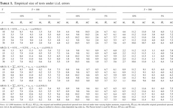
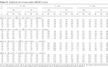
Tables 1 and 2 report the empirical rejection rates of the tests under

at the 10% and 5% significance levels, using the asymptotic theory. We first consider the unmodified test

. When the DGP is an AR(d) process with i.i.d. errors,

underrejects

severely at both the 10% and 5% levels (particularly for larger d), even when T = 500. When the DGP is an AR(d) process with ARCH errors,

also shows underrejection (particularly when T = 100), but the sizes are better than under DGPs with i.i.d. errors when T ≥ 250, and they improve as T increases. Overall, as the lag order d of the AR model increases,

displays more severe underrejection (except for the case at the 5% level and when T = 500), thus confirming our conjecture.

Empirical size of tests under i.i.d. errors

Empirical size of tests under ARCH(1) errors

To investigate whether the underrejection of

is due to the impact of parameter estimation uncertainty, we also report the rejection rates of the infeasible test statistic

of (2.13) that uses the true errors {ε_t} rather than the estimated model residuals

. When {ε_t} is i.i.d.,

outperforms

for all sample sizes T, and its sizes are reasonable and are robust to the choice of the preliminary lag order p. Note that the rejection rates of

remain unchanged when the order of the AR(d) model increases, because

does not use the estimated model residuals

. When {ε_t} is ARCH(1),

shows some underrejections when T = 100, but its sizes become reasonable when T ≥ 250. For all sample sizes T,

outperforms

. These results confirm our theory that parameter estimation uncertainty has nontrivial impact on

in finite samples. In particular, parameter estimation is like a calibration that makes the estimated model residuals look more like an m.d.s., leading to underrejection of the test.

For each sample size T and each preliminary lag order p, the means of the data-driven lag

are the same or very similar for all

,

, and

, regardless of the order of the AR(d) model and the types (i.i.d. or ARCH(1)) of the errors. When the preliminary lag p changes from 10 to 30, the means of

range from 4.6 to 7.2 for T = 100, from 5.5 to 7.2 for T = 250, and from 6.2 to 7.3 for T = 500. These results indicate relative robustness of

to the choice of p.

For the Bartlett kernel, the range of the means of

is wider, from 6.3 to 17.5 when T = 100, from 6.4 to 17.8 for T = 250, and from 6.6 to 18.0 when T = 500. This is apparently due to different bandwidth rules: for the Bartlett kernel,

, and for the Parzen kernel,

. Nevertheless, the sizes of the tests using the Bartlett kernel are similar to the sizes of the tests using the Parzen kernel. These results are available from the authors upon request.

We now turn to the modified test

to examine whether the Wooldridge (1990a) device can effectively reduce the impact of parameter estimation uncertainty on the sizes of the test. For T = 100,

shows some overrejections when the order d of the AR(d) model is relatively large. However, it has reasonable sizes under all DGPs for T ≥ 250. The

test performs more similarly to the infeasible test

than

when T = 100, and when T ≥ 250,

and

perform more or less similarly. These results indicate the relative robustness of the modified test

to parameter estimation uncertainty, illustrating the merits of applying the Wooldridge (1990a) device to the generalized spectral tests.

Next, we turn to the power of the tests

and

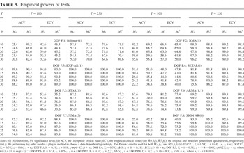
. Table 3 reports the empirical rejection rates of the tests at the 5% significance level under DGPs P.1–P.8 using asymptotic and empirical critical values, respectively. For the power using asymptotic critical values,

is more powerful than or equally powerful to

under all scenarios, which is not surprising at all given the fact that

tends to underreject under

. Under DGPs P.1 (bilinear(1)), P.2 (NMA(1)), P.4 (SETAR(1)) and P.8 (SIGN AR(6)),

has substantially lower power than

when T = 100, although its power increases as the sample size T increases and catches up with that of

when T = 250. This is consistent with the substantial underrejection of

due to the impact of parameter estimation uncertainty. Under DGPs P.2 (NMA(1)), P.3 (EXP-AR(1)), P.6 (ARMA(1,1)), P.7 (NMA(5)), and P.8 (SIGN AR(6)), both

and

have unit power except for one scenario when T = 250.

Empirical powers of tests

We now compare the powers of the tests using empirical critical values, which provide fair comparison of different tests on an equal ground. The empirical critical values are obtained under AR(1)-i.i.d. Under DGP P.1 (bilinear(1)),

is a bit more powerful than

when T = 100. They have equal or similar power when T = 250. The power of

is relatively more robust to the choice of the preliminary lag order p than that of

. Under DGP P.2 (NMA(1)),

and

have roughly equal power. The power of

and

is rather robust to the choice of the preliminary lag order p when T = 250.

Under DGP P.3 (EXP-AR(1)),

is slightly less powerful than

when T = 100. When T = 250,

and

have the same unit power. Also, the power of both tests is robust to the choice of preliminary lag order p. Under DGP P.4 (SETAR(1)),

and

also have roughly equal powers for each sample size T.

Under DGP P.5 (STAR(1)),

is less powerful than

, particularly when T = 100, but the power of

increases rapidly as T increases. Under DGP P.6 (ARMA(1,1)), the power of

is slightly smaller than that of

, and it quickly increases as T increases. When T = 250,

and

are equally powerful, and their powers are close to unity.

Under DGP P.7 (NMA(5)),

is slightly less powerful than

when T = 100, but its power quickly catches up with that of

when T = 250. When T = 250, both tests have unit power. Under DGP P.8 (SIGN AR(6)), both

and

are equally powerful for both sample sizes, and they have unit power when T = 250.

We note that there exist substantial or significant differences between the power of

using the asymptotic critical value and the power of

using the empirical critical value. In particular, the power of

using asymptotic critical value is lower than that of

using empirical critical value. In contrast, the power of

using asymptotic critical value is similar to that of

using empirical critical value in all cases.

In summary, we have observed the following stylized facts.

• The empirical sizes of the original
  
  test are substantially lower than the nominal significance levels, because of the impact of parameter estimation uncertainty. The underrejection is more severe under homoskedastic errors and with more estimated autoregressive parameters. On the other hand, the Wooldridge (1990a) device can effectively reduce the impact of parameter estimation uncertainty; the empirical sizes of the modified
  
  test are reasonable in most cases, especially when the sample size becomes moderately large. Its sizes are slightly larger than the corresponding significance levels when the preliminary lag order p is small, but they improve as both the preliminary lag order p and the sample size T increase.
• As the lag order d of the AR(d) model increases, i.e., the number of estimated autoregressive parameters increases,
  
  shows more severe underrejections. In contrast,
  
  is relatively robust to parameter estimation uncertainty and the number of estimated autoregressive parameters in most cases.
• For the power using asymptotic critical values,
  
  is always more powerful than
  
  , and the power of
  
  is more robust to the choice of the preliminary lag order p than that of
  
  in many cases.
• When using empirical critical values, the
  
  test is not always as powerful as the
  
  test, but it has similar power to
  
  in most cases, particularly when the sample size is moderately large. There is not much power loss for the modified test, although its size has been significantly improved. Both tests have omnibus power against all eight DGPs provided the sample size is sufficiently large. They require no knowledge of the lag structure of the potential alternative.
• There exist some substantial differences between the power of
  
  using the asymptotic critical value and the power of
  
  using the empirical critical value. In particular, the power of
  
  using asymptotic critical values is always lower than the power of
  
  using empirical critical values, sometime rather substantially. In contrast, the powers of
  
  using asymptotic and empirical critical values are more or less similar.