1 Introduction
Helical vortices appear both in nature and in connection with various fluid dynamic applications, and many flow visualizations have shown that the flow behaviour in the near wake of rotors essentially is determined by concentrated helical vortices. This includes vortices emanating from the blade tips of wind turbines (Vermeer, Sørensen & Crespo Reference Vermeer, Sørensen and Crespo2003), helicopters (Leishman Reference Leishman2006) and propellers (Felli & Camussi Reference Felli, Camussi and Di Felice2011; Sørensen Reference Sørensen2011). Assuming ideally that the shapes of the helical tip vortices are kept unchanged when progressing into the wake, it is possible to derive analytical solutions describing the flow field (Okulov & Sørensen Reference Okulov and Sørensen2010; Okulov, Sørensen & Wood Reference Okulov, Sørensen and Wood2015b ). These vortex solutions together with a simplification of the rotor as an actuator disc enabled appropriate approximations for blade design, leading to classical design proposals (see Van Kuik, Sørensen & Okulov Reference Van Kuik, Sørensen and Okulov2015 or Sørensen et al. Reference Sørensen, Okulov, Mikkelsen, Naumov and Litvinov2016). Further downstream in the wake, however, the helical vortices become unstable and break down into turbulence (Felli & Camussi Reference Felli, Camussi and Di Felice2011; Quaranta, Bolnot & Leweke Reference Quaranta, Bolnot and Leweke2015; Sarmast et al. Reference Sarmast, Dadfar, Mikkelsen, Schlatter, Ivanell, Sørensen and Henningson2014). To understand and predict the stability properties of helical vortices and their subsequent transition to turbulence, it is important to be able to describe the flow structures of the undisturbed vortices (Sørensen et al. Reference Sørensen, Mikkelsen, Sarmast, Ivanell and Henningson2014).
Widnall (Reference Widnall1972) and Gupta & Loewy (Reference Gupta and Loewy1974) were the first to utilize a Rankine vortex model (constant-vorticity core) as a basis for studying the stability of helical vortices. Fukumoto & Miyazaki (Reference Fukumoto and Miyazaki1991) later extended this work by including an axial flow component along the vortex core. Recently, Quaranta et al. (Reference Quaranta, Bolnot and Leweke2015) experimentally discovered and improved the models by introducing a more realistic Gaussian vorticity distribution with an additional axial flow in the core. The proposed scaling behaviour and the concept of helical self-similarity including both the axial and the azimuthal velocity profiles in the helical vortex core are expected to provide a more correct basis for future studies on vortex instability.
A main problem associated with near-wake studies is to understand the downstream evolution of the tip vortex core, where the continuous growth in the vortex core strongly affects the global vortex stability. A classic example of this is the self-similar temporal growth of the Lamb–Oseen vortex (Saffman Reference Saffman1992), for which a time–spatial relation for the downstream development is established using a molecular diffusion model. Ali & Abid (Reference Ali and Abid2014) paid particular attention to the swirling form of the helical tip vortex to investigate the degree of resemblance between the helical vortex core and the Lamb–Oseen vortex. For this purpose, they applied a numerical solution of the Navier–Stokes equations for different low Reynolds numbers, using the actuator line approximation (Sørensen & Shen Reference Sørensen and Shen2002), to estimate the vortex core evolution due to molecular diffusion as a function of vortex age. The evolution of velocity and vorticity in the core of the helical tip vortex, generated by a single-bladed rotor, was compared to the solution of the Lamb–Oseen vortex assuming a molecular diffusive expansion of the rectilinear vortex core. The authors (Ali & Abid Reference Ali and Abid2014) used appropriate similarity variables and scaling to remove the local and global non-axisymmetric effect on the helical vortex topology, and reached a good agreement with the axisymmetric solution of the Lamb–Oseen vortex. Ultimately, the numerical investigation showed that the diffusive evolution of the helical vortex core with good accuracy coincides with the molecular diffusive evolution of the Lamb–Oseen vortex. However, this process, depending only on kinematic viscosity, is very slow and disagrees with observations of practical swirling flows, where a significantly greater expansion of the vortex core takes place due to turbulent diffusion. Nevertheless, Ali & Abid (Reference Ali and Abid2014) demonstrated the possibility of employing special variables and scaling to remove the local and global non-axisymmetric effects in order to compare vortex cores of helical and rectilinear vortices.
Recently, considering the evolution of the tip vortex core in different cross-sections behind an immobile vortex generator, and by scaling the local radius of the vortex core and the local helical pitch of the vortex lines filling the core, Velte, Hansen & Okulov (Reference Velte, Hansen and Okulov2009) found a complete correspondence between the local axial and azimuthal velocity profiles. This correlation, referred to as ‘local helical symmetry’, was originally introduced by Alekseenko, Kuibin & Okulov (Reference Alekseenko, Kuibin and Okulov2007) to describe main parameters of swirling flows.
The current study is based on experimental observations from current and previous studies of tip vortices behind a three-bladed rotor (Naumov et al.
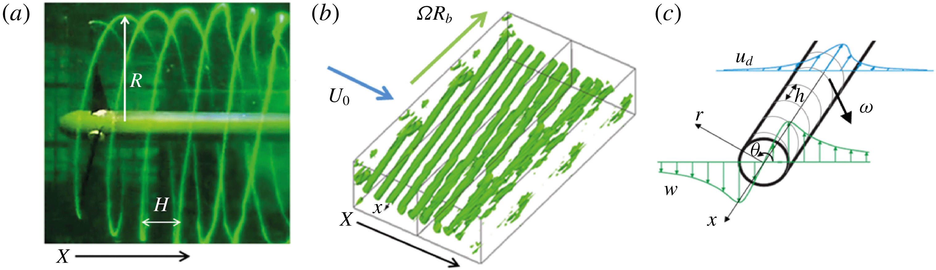
Reference Naumov, Rahmanov, Okulov, Velte, Meyer and Mikkelsen2012, Reference Naumov, Mikkelsen, Okulov and Sørensen2014). Rotating blades generate helical vortices at the tip of the blades (figure 1
a). In global terms, the helical system is described by a vortex pitch
 $H$
and a tip vortex radius
 $R$
. The local coordinates (
 $x,r,\unicode[STIX]{x1D703}$
) are introduced to study the development of the individual vortex core (see figure 1
b,c). Note that
 $u_{d}$
in the figure denotes the deficit velocity. The objective is to deduce the possible existence of a general relation between the local axial velocity
 $u$
and the local azimuthal velocity
 $w$
in all cross-sections of a tip vortex, or, in other words, to investigate the possibility of self-similar behaviour along the vortex axis
 $x$
. This procedure of combining local-scale similarity with the downstream development of the vortex core will in the following be referred to as ‘helical self-similarity’.
Visualization of tip vortices behind a rotor (a), horizontal scanning of tip vortices (b) and local coordinate system (
 $r,\unicode[STIX]{x1D703},x$
) of a single tip vortex (c).

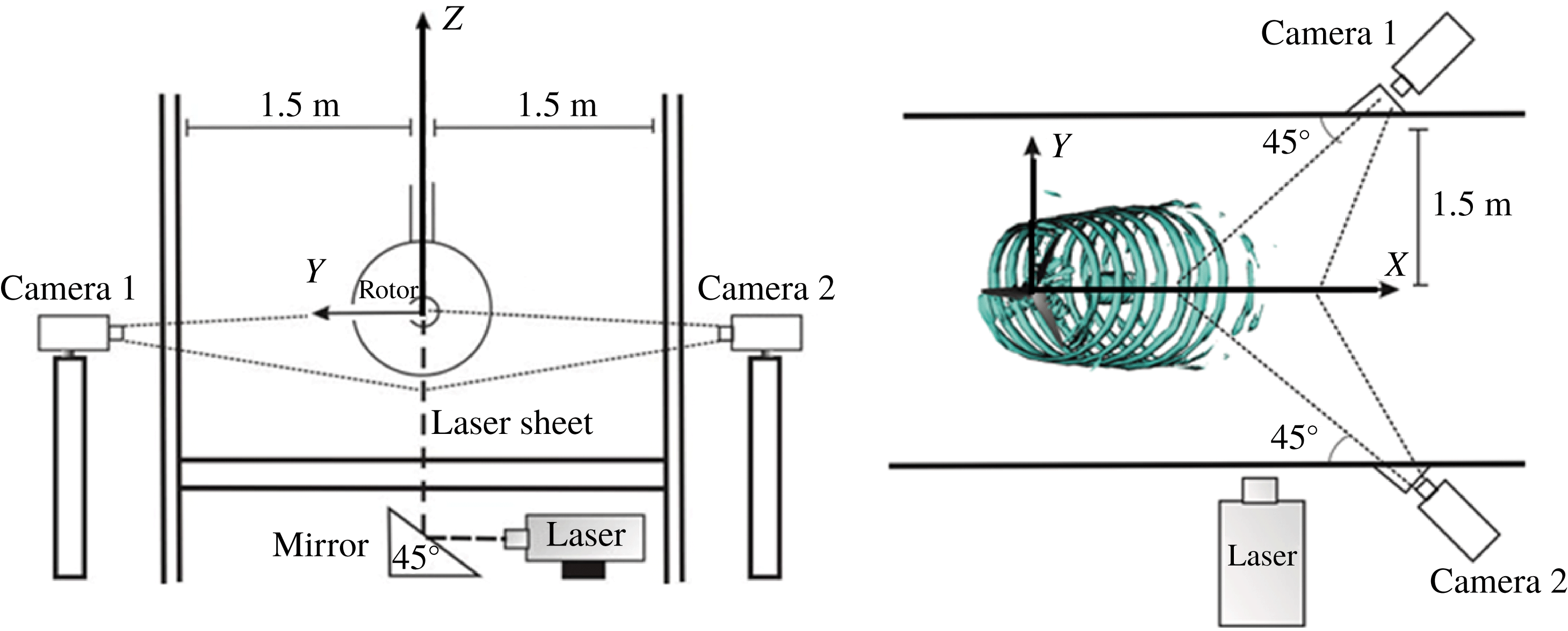
Sketch of PIV measurements in the two cross-sections of the flume and definition of the global coordinate system
 $(X,Y,Z)$
.

2 Experimental set-up and method
2.1 Experimental set-up and measurement technique
The basis for the work is a series of experiments of tip vortices generated on a model of a horizontal axis wind turbine. The experiments were carried out in a water flume of length 35 m and width 3 m, and a water level of about 0.9 m (figure 2). The temperature of the water was
 $20\,^{\circ }\text{C}$
. The test section of the flume is equipped with transparent walls at a distance of 20 m from the flume inlet. The free-flow velocity in the test section of the flume was about
 $U_{0}=0.6~\text{m}~\text{s}^{-1}$
with a water flow rate of
 $1.5~\text{m}^{3}~\text{s}^{-1}$
. The allowed deviations in the flow rate were less than 2 %. The small boundary layer thickness (
 ${\approx}0.2$
m) and the slight level of turbulent pulsations (
 ${\sim}2.5\,\%$
) for the undisturbed flow provide a nearly uniform incoming flow in the test area in the middle of the flume, according to previous data (Okulov et al.
Reference Okulov, Naumov, Mikkelsen, Kabardin and Sørensen2014).
The three-bladed model rotor has a diameter of 0.376 m, and is equipped with blades of length 159 mm consisting of SD7003 airfoil sections (Selig et al.
Reference Selig, Guglielmo, Broeren and Giguere1995). The shape and pitch setting of the blades were determined using the aerodynamic design theory of Glauert (Okulov & Mikkelsen Reference Okulov, Mikkelsen, Litvinov and Naumov2015a
) for optimum operating conditions with a constant design lift coefficient along the span (
 $C_{L}=0.8$
). The rotor was designed to operate optimally at a tip speed ratio
 $\unicode[STIX]{x1D706}=5$
, where
 $\unicode[STIX]{x1D706}=\unicode[STIX]{x1D6FA}R_{b}/U_{0}$
, with
 $\unicode[STIX]{x1D6FA}$
being the rotor angular velocity,
 $R_{b}$
the rotor radius and
 $U_{0}$
the initial velocity in the flume. The Reynolds number for all experiments was about 20 000, calculated as
 $Re=\unicode[STIX]{x1D70C}b\unicode[STIX]{x1D6FA}R_{b}/\unicode[STIX]{x1D707}$
. Here
 $b=0.1$
is the chord length of the blade, and
 $\unicode[STIX]{x1D70C}$
and
 $\unicode[STIX]{x1D707}$
are the density and dynamic viscosity of the working fluid (tap water), respectively.
The rotor is located at a height of 0.5 m from the flume bottom and at a distance of 1.5 m from the flume walls (see figure 2), thus avoiding the influence of the boundary layer, whose thickness is less 20 cm from the bottom and the walls of the flume. The ratio between the rotor area (
 $0.111~\text{m}^{2}$
) and the area of the flume cross-section (
 $3~\text{m}^{2}$
) is 3.7 %. Therefore, blockage effects are very small and no corrections are made. The rotor was driven by a JVL Industri Elektronik MAC140 servo motor, which was operated at a constant rotational speed within 1.5 % accuracy. The torque was transmitted by the external gear at the axis of each rotor.
The global coordinate system is defined in figure 2. The origin of the coordinate system is chosen as the cross-section of the rotor axis and the rotor plane, with
 $X$
pointing in the axial direction,
 $Y$
in the wall-normal direction and
 $Z$
in the spanwise direction (see figure 2). The velocity components in
 $OX$
,
 $OY$
and
 $OZ$
directions are denoted
 $U$
,
 $V$
and
 $W$
, respectively. The local coordinates (
 $x,r,\unicode[STIX]{x1D703}$
) were introduced to study the development of the individual vortex core (see figure 1
b,c), where
 $x$
follows a central line of the tip vortices, and
 $h$
denotes the internal tip vortex pitch with
 $l=h/2\unicode[STIX]{x03C0}$
. The tip vortices expand in the wake from the rotor blades to a radius
 $R\approx 1.22R_{b}$
(Okulov et al.
Reference Okulov, Naumov, Mikkelsen, Kabardin and Sørensen2014). The local velocity field is given as
 $(u,v,w)$
, with
 $u_{0}=u(x,0)$
denoting the vortex centre, and
 $u_{d}(x,r)=(u(x,r)-u_{0}(x))$
defining the deficit velocity.
The flow field was measured using a Dantec stereoscopic particle image velocimetry (PIV) system, which gives all three velocity components (
 $U,V,W$
) throughout the window of the light sheet. An Nd:YAG laser was used as light source with the following characteristics: 120 mJ of energy in a single pulse, a wavelength of 532 nm and an operational frequency of 15 Hz. A 2 mm thick vertical light sheet was sent into the channel from the bottom in the same plane as the rotor axis (figure 2). The processing of the images resulted in three downstream windows to yield the local velocity field. The final size of the full three-dimensional velocity field for investigating the helical tip vortex was 1.03 m
 $\times$
0.29 m. The images in the measuring windows were recorded by two Dantec HiSense II cameras with
 $1344\times 1024$
pixel resolution. The cameras were placed perpendicularly to each other on the different sides of the flume with an angle of
 $45^{\circ }$
to the walls (figure 2). Water-filled optical prisms were installed between the cameras, and the focus plane was adjusted using Scheimpflug adapters. The three-dimensional velocity field in each testing window was calculated using Dantec Dynamic Studio 2.21. The stereoscopic PIV system was calibrated using a target with a well-defined dot pattern which was translated and registered by the cameras in a number of well-defined positions at the light sheet. The measuring error of stereoscopic PIV velocity measurements was at the level of 3 %–5 %.
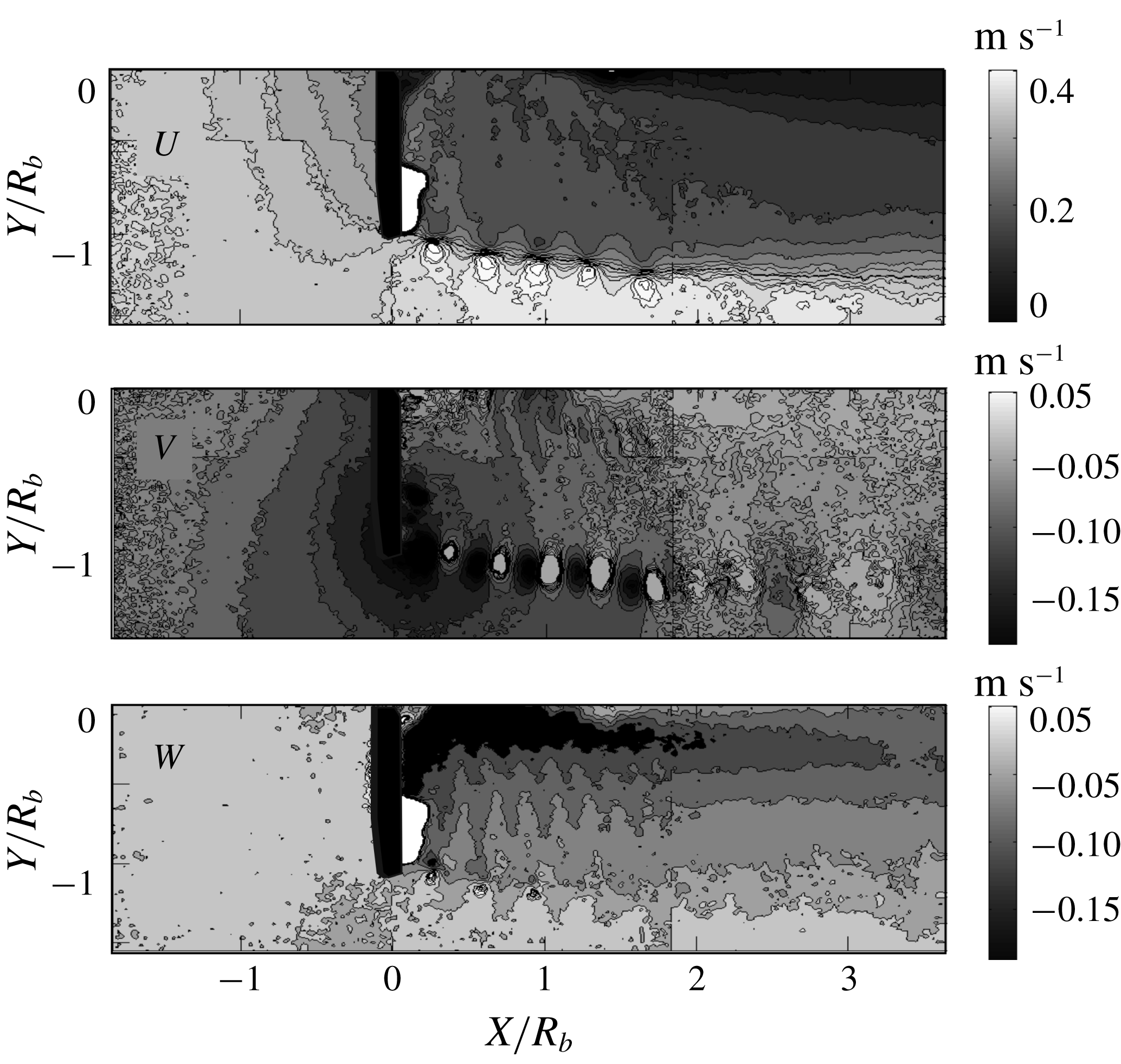
The iso-contours of the global axial (
 $U$
), radial (
 $V$
) and azimuthal (
 $W$
) velocities at
 $\unicode[STIX]{x1D706}=5$
.

The synchronized velocity field in each window was obtained by phase averaging of 200 PIV velocity realizations, which were recorded in the moment of a triggered signal by a light pulse for each complete rotation of the rotor. An angular encoder (LIKA ASR58) with angular resolution of
 $0.1^{\circ }$
, installed on the rotor hub, triggered a pulse when one of the blades passed through the light sheet. The stochastic errors vanish by this phase averaging. Moreover, this approach eliminates the drifting error due to non-stationary flow regimes. The time interval between consecutive PIV images was based on the frequency of the rotor rotation, which for
 $\unicode[STIX]{x1D706}=5$
was
 $T=(1/2.18)$
s.
2.2 Vortex core determination
Figure 3 shows the phase-averaged distributions of the axial
 $(U)$
, radial
 $(V)$
and azimuthal
 $(W)$
velocity components of the flow for
 $\unicode[STIX]{x1D706}=5$
. The angles of the blade rotation from which the synchronization was made in the experiments were verified in the range
 $\unicode[STIX]{x1D6FC}=0$
–
 $105^{\circ }$
, with steps of
 $15^{\circ }$
. The vorticity field was calculated from the velocity field in all cross-sections (figures 3 and 4). The plots demonstrate that the tip vortices appear as regular vortex structures with clear cores. The vortex cores are destroyed at a distance in the range between
 $1.8R$
and
 $3.6R$
due to their mutual interaction. The vorticity cross-section with the clearest vortex cores was used to determine the centres of the tip vortices (
 $Y_{c}$
,
 $Z_{c}$
) in the PIV plane. The centres of the tip vortices were determined from an algorithm based on the centre of mass. The vortex core is described in a rectangular domain,
 $A$
, defined as
 $Y-Y_{c}\in [-h/2,h/2]$
and
 $Z-Z_{c}\in [-R_{b}/2,R_{b}/2]$
. The circulation
 $\unicode[STIX]{x1D6E4}$
of the vortex core is determined by integration of the vorticity:
 $$\begin{eqnarray}\unicode[STIX]{x1D6E4}=\int _{A}\unicode[STIX]{x1D714}_{x}\,\text{d}A.\end{eqnarray}$$
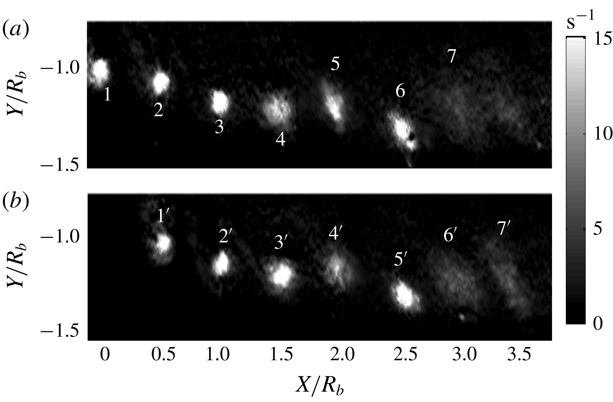
The vorticity maps of tip vortex cross-sections for the rotor synchronizations at an angle of (a)
 $0^{\circ }$
and (b)
 $105^{\circ }$
. Examples of the local coordinates and numbering of the vortex cross-sections.

The images of the tip vortex cores along the wake were from left to right numbered 1 to 9. Hence, the vortex cores 1, 4, 7 and
 $1^{\prime }$
,
 $4^{\prime }$
,
 $7^{\prime }$
; cores 2, 5, 8 and
 $2^{\prime }$
,
 $5^{\prime }$
,
 $8^{\prime }$
; cores 3, 6, 9 and
 $3^{\prime }$
,
 $6^{\prime }$
,
 $9^{\prime }$
correspond to the cross-section of the tip vortices behind the first, second and third blades, respectively. The vorticity plots also show that blurring of the vortex core takes place. The first six images of the core have a strong concentration of vorticity and are approximately located at equal distances from each other, whereas the vorticity concentrations of cores 7, 8 and 9 are seen to be less dense and the cores are displaced further from each other. Based on the observations, the development of the helical vortex cores will be analysed in the next section.
3 Helical self-similarity of the vortex cores
Self-similarity occurs when the velocity profile can be brought into congruence by a simple scale factor. As a consequence, the dynamical equations are usually reduced to a single geometrical variable in their functional. The idea of self-similarity in fluid flows appears to have been applied for the first time by Blasius in 1908 for laminar boundary layers. Turbulent wakes are known to develop self-similarly downstream sufficiently far away from the obstacles that generate them (e.g. George Reference George2012 and references therein). Some vortex wakes, whose longitudinal variables achieve similarity, can further be dependent on similarity conditions in the azimuthal direction too. The existence of similarity between axial and azimuthal velocity fields leads us in the current investigation to introduce the concept of helical self-preservation for turbulent vortex wakes.
As a starting point for our analysis of the interior of helical vortices, we employ the solution of the Lamb–Oseen vortex (Lamb Reference Lamb1932). This solution describes the decay of the azimuthal velocity
 $w$
, or the associated vorticity distribution
 $\unicode[STIX]{x1D714}_{x}$
, in a longitudinal vortex:
 $$\begin{eqnarray}\left.\begin{array}{@{}c@{}}\displaystyle w(r,t)=\frac{\unicode[STIX]{x1D6E4}}{2\unicode[STIX]{x03C0}\,r}\left(1-\exp \left(-\frac{r^{2}}{r_{c}^{2}(t)}\right)\right)\quad \text{or}\\ \displaystyle \unicode[STIX]{x1D714}_{x}(r,t)=\frac{\unicode[STIX]{x1D6E4}}{\unicode[STIX]{x03C0}\,r_{c}(t)^{2}}\exp \left(-\frac{r^{2}}{r_{c}^{2}(t)}\right),\quad r_{c}(t)=\sqrt{4t\unicode[STIX]{x1D708}_{k}},\end{array}\right\}\end{eqnarray}$$
where
 $\unicode[STIX]{x1D6E4}$
is the vortex circulation,
 $r$
is the local radial coordinate from the centre of the vortex core,
 $r_{c}(t)$
is the radius of the vortex core and
 $\unicode[STIX]{x1D708}_{k}$
is the kinematic viscosity. A similar model was used by Ali & Abid (Reference Ali and Abid2014) for comparison with results from Navier–Stokes simulations of helical vortices. In their comparison they proposed to use the radius growth of the Lamb–Oseen vortex
 $$\begin{eqnarray}\unicode[STIX]{x0394}r_{c}^{2}\equiv r_{c}^{2}(t)-r_{c}^{2}(t_{0})=4(t-t_{0})\,\unicode[STIX]{x1D708}_{k}\end{eqnarray}$$
as a model for the diffusion process of a helical vortex filament.
Another important element in our model is the concept of a two-dimensional helical symmetry, proposed by Landman (Reference Landman1990) and Dritschel (Reference Dritschel1991). Assuming a helical vortex configuration consisting of a single vortex with constant pitch (
 $h=2\unicode[STIX]{x03C0}l$
) and core radius (
 $r_{c}=\text{const.}$
), the vorticity only depends on a single variable,
 $r$
, and the relation between the axial and azimuthal vorticity components is given simply as the ratio between the radial position and the helical pitch:
 $$\begin{eqnarray}\unicode[STIX]{x1D714}_{x}=\frac{\unicode[STIX]{x1D6E4}}{\unicode[STIX]{x03C0}\;r^{2}}\exp \left(-\frac{r^{2}}{r_{c}^{2}}\right),\quad \unicode[STIX]{x1D714}_{\unicode[STIX]{x1D703}}=r\unicode[STIX]{x1D714}_{x}/l,\quad \unicode[STIX]{x1D714}_{r}=0.\end{eqnarray}$$
A partial case of an axisymmetric flow with helical symmetry of the vorticity field (Kuibin & Okulov Reference Kuibin and Okulov1996) is
 $$\begin{eqnarray}w=\frac{\unicode[STIX]{x1D6E4}}{2\unicode[STIX]{x03C0}\,r}\left[1-\exp \left(-\frac{r^{2}}{r_{c}^{2}}\right)\right],\quad u=u_{0}-\frac{\unicode[STIX]{x1D6E4}}{2\unicode[STIX]{x03C0}\,l}\left[1-\exp \left(-\frac{r^{2}}{r_{c}^{2}}\right)\right],\end{eqnarray}$$
where
 $u$
is the axial velocity component,
 $w$
is the tangential component and
 $u_{0}$
is the axial velocity at the centre of the vortex core. From (3.4) one gets a similar expression for the correlation between the velocities:
 $$\begin{eqnarray}u+\frac{r}{l}w=u_{0}.\end{eqnarray}$$
Using this expression, local helical symmetry for the average velocity has been found to exist in various swirling flow configurations (Martemianov & Okulov Reference Martemianov and Okulov2004; Alekseenko et al. Reference Alekseenko, Kuibin and Okulov2007; Velte et al. Reference Velte, Hansen and Okulov2009).
At a first view, the velocity field in the form of (3.4) corresponds to the self-similar solution of the Batchelor vortex. For two trailing vortices located downstream from a wing, assuming that the core diameter is an order of magnitude smaller than the distance between the vortices, Batchelor (Reference Batchelor1964) proposed to replace the temporal dependence
 $t$
in the diffusion process (3.2) via a space correlation
 $x/B$
 $$\begin{eqnarray}\unicode[STIX]{x0394}r_{c}^{2}\equiv r_{c}^{2}(x)-r_{c}^{2}(x_{0})=4(x-x_{0})\unicode[STIX]{x1D708}_{t}/B,\end{eqnarray}$$
where
 $B$
is a characteristic velocity and
 $\unicode[STIX]{x1D708}_{t}$
is the turbulent viscosity, which may be identical to the one of the incoming turbulence flow. Batchelor furthermore derived the following form of the azimuthal and axial velocity components:
 $$\begin{eqnarray}rw(x,r)=C_{0}(1-\text{e}^{-\unicode[STIX]{x1D702}}),\quad u(x,r)=B-D\text{e}^{-\unicode[STIX]{x1D702}}/8\unicode[STIX]{x03C0}\,x\unicode[STIX]{x1D708}_{t},\end{eqnarray}$$
where
 $\unicode[STIX]{x1D702}=Br^{2}/4x\unicode[STIX]{x1D708}_{t}$
, the constant
 $C_{0}\equiv \unicode[STIX]{x1D6E4}/2\unicode[STIX]{x03C0}$
represents
 $1/2\unicode[STIX]{x03C0}$
times the flow circulation and
 $D$
describes the ‘drag’ of the body divided by density
 $\unicode[STIX]{x1D70C}$
. It should be mentioned that (3.7) originally was applied to an isolated longitudinal vortex. In order to apply (3.7) to helical vortices, the distance between the turns of the tip vortices is assumed to be large.
A universal solution including both helical symmetry and self-similar expansion of the vortex core is still unknown for longitudinal as well as for helical vortices, but as an empirical model together with (3.6), we propose a combination of (3.4) and (3.7) in the form
 $$\begin{eqnarray}w=\frac{\unicode[STIX]{x1D6E4}}{2\unicode[STIX]{x03C0}\,r}\left[1-\exp \left(-\frac{r^{2}}{r_{c}^{2}(x)}\right)\right],\quad u=B-\frac{\unicode[STIX]{x1D6E4}}{2\unicode[STIX]{x03C0}\,l\left(x\right)}\left[1-\exp \left(-\frac{r^{2}}{r_{c}^{2}(x)}\right)\right].\end{eqnarray}$$
This new model only requires empirical knowledge or experimental calibration of some few flow parameters: vortex circulation,
 $\unicode[STIX]{x1D6E4}$
, helical pitch,
 $l=l(x)$
, advection velocity along the vortex axis,
 $B$
, and growth factor of the vortex core,
 $r_{c}$
. All the mentioned parameters can be determined experimentally by using PIV measurements of the velocity field (figure 3) together with the reconstructed vorticity field (figure 4).
The last images in figure 4 show a non-circular form of the vortex cores, which reveals the existence of an asymmetry of the global helix in a planar cross-section. By averaging the profiles, however, these asymmetric changes of the circular vortex core repeated from cross-section to cross-section have a marginal influence on the regular vortex evolution. The averaging is allowed by the linear correlation between the two velocities in (3.5). In accordance with this, azimuthally averaged local velocities and vorticity are used in the following:
 $$\begin{eqnarray}\left.\begin{array}{@{}c@{}}\displaystyle \unicode[STIX]{x1D714}_{x}(x,r)=\frac{1}{2\unicode[STIX]{x03C0}}\int _{0}^{2\unicode[STIX]{x03C0}}\unicode[STIX]{x1D714}_{x}(x,r,\unicode[STIX]{x1D703})\,\text{d}\unicode[STIX]{x1D703};\quad w(x,r)=\frac{1}{2\unicode[STIX]{x03C0}}\int _{0}^{2\unicode[STIX]{x03C0}}w(x,r,\unicode[STIX]{x1D703})\,\text{d}\unicode[STIX]{x1D703};\\ \displaystyle u(x,r)=\frac{1}{2\unicode[STIX]{x03C0}}\int _{0}^{2\unicode[STIX]{x03C0}}u(x,r,\unicode[STIX]{x1D703})\,\text{d}\unicode[STIX]{x1D703}.\end{array}\right\}\end{eqnarray}$$
The scaling radial similarity variable for the first, fourth and seventh vortex core (figure 4) is determined as the value of the radius,
 $r_{c}$
. The value of
 $r_{c}$
is taken at the radius value where the azimuthal velocity
 $w$
attains its maximum. Therefore, the scaled values of the profiles (3.9) for a fixed axial position,
 $x$
, or vortex number, can be recalculated by
 $$\begin{eqnarray}\left.\begin{array}{@{}c@{}}\displaystyle \tilde{\unicode[STIX]{x1D714}}_{x}(x,r/r_{c}(x))=\frac{\unicode[STIX]{x1D714}_{x}(x,r/r_{c}(x))}{\max _{r}\,\unicode[STIX]{x1D714}_{x}(x,r)},\\ \displaystyle \tilde{w}(x,r/r_{c}(x))=\frac{w(x,r/r_{c}(x))}{\max _{r}\,w(x,r)},\\ \displaystyle \tilde{u} _{d}(x,r/r_{c}(x))=\frac{u_{d}(x,r/r_{c}(x))}{\max _{r}\,u_{d}(x,r)},\end{array}\right\}\end{eqnarray}$$
where
 $\max _{r}\,u_{d}(x,r)$
requires a special consideration, as will be shown in the next section.
4 Helical vortex development
The evolution of the local cores of the helical tip vortices was investigated through velocity fields measured by stereoscopic PIV, as described in § 2. Two global velocity plots with the blade oriented to the bottom at angles of
 $0^{\circ }$
and
 $105^{\circ }$
from the vertical axis were studied. The two cross-sections reproduce seven well-visible tip vortex cores, with the cores numbered by 1,
 $1^{\prime }$
, 4,
 $4^{\prime }$
, 7 and
 $7^{\prime }$
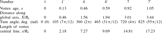
, respectively, to keep track of the tip vortex trailed from the same blade (figure 4). The cross-sections may alternatively be described by the total angle they have travelled downstream, by their vortex age or by their axial position measured in rotor radii (see table 1).
(
 $a$
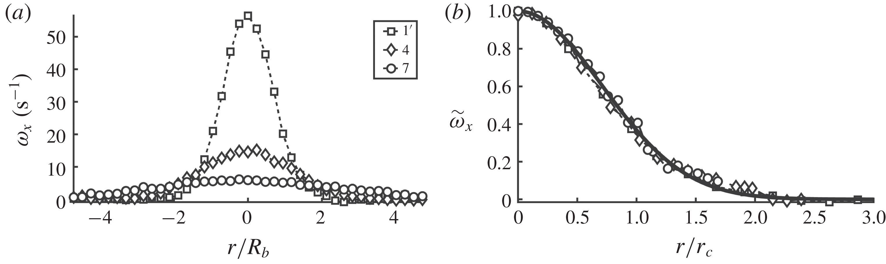
) Lines with symbols indicate the original PIV profiles of the local vorticity in the core at different cross-sections of the tested helical vortex. (
 $b$
) Comparison of the same half profiles, scaled by (4.1), with the analytical non-dimensional solution (3.4) shown by a solid line.

Position of cross-sections of tip vortex cores.

The vortex age of a section of the tip vortex is calculated via the turn angles and the frequency of the rotor rotation, which for
 $\unicode[STIX]{x1D706}=5$
is equal to 2.18 Hz. The coordinate
 $x$
was calculated as in Quaranta et al. (Reference Quaranta, Bolnot and Leweke2015). The intervals were selected to avoid any blade influence in the second core cross-section at the
 $105^{\circ }$
turn and to include the last vortex at the
 $825^{\circ }$
turn just before the helical vortex is destroyed. Indeed, the vortex core in the first position at
 $0^{\circ }$
near the rotor blade is strongly influenced by the rotor blade and the vortex generation process. In spite of this, for further analysis and to complete the picture, we have included both extreme positions (1 and
 $7^{\prime }$
) in the analysis.
As a first step, a local coordinate system, (
 $x,r,\unicode[STIX]{x1D703}$
), with the origin located at the centre of each cross-section of the tested tip vortex was introduced. Examples of axial vorticity profiles at cross-sections
 $1^{\prime }$
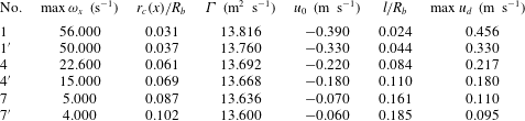
, 4, 7, corrected for minor asymmetries by azimuthal averaging (3.9), are shown in figure 5(a). The same profiles scaled by (3.10) are shown in figure 5(b) and compared to the analytical solution (3.3). The scaling parameters of the investigated vorticity and velocity profiles are presented in table 2.
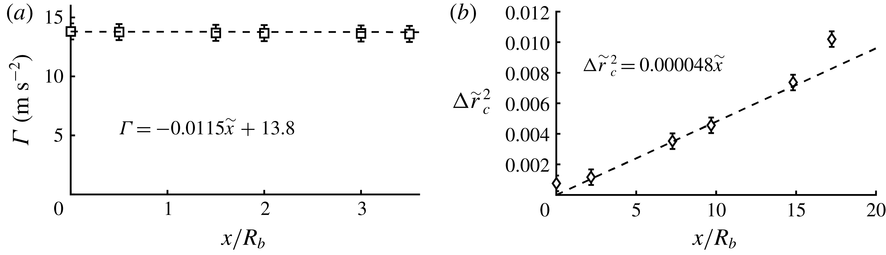
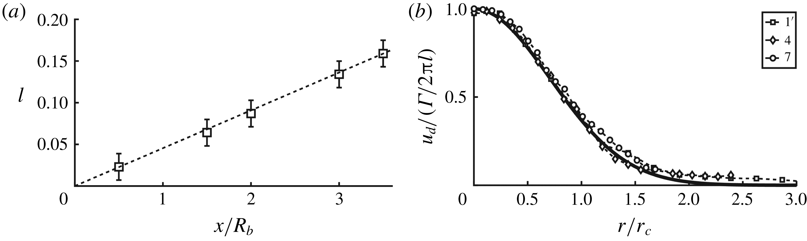
Downstream distribution of circulation (
 $a$
) and evolution of vortex core radius (
 $b$
) along the helical tip vortex in the different cross-sections. The lines are linear fittings.

Parameters of the vortex evolutions.

As seen in figure 6, the circulation does not change along the tip vortex (figure 6 a), whereas the evolution of the vortex core shows an expansion (figure 6 b) that follows the law of molecular diffusion (3.6), but at a higher rate corresponding to a turbulent viscosity, which is about 2000 times higher than the molecular viscosity. The relative error for circulation and the vortex core radius was based on PIV velocity measuring error and was estimated to be 12 % for the circulation and 10 % for the vortex core radius. A suitable presentation of (3.6) gives the non-dimensional form of the solution:
 $$\begin{eqnarray}\unicode[STIX]{x0394}\tilde{r}_{c}^{2}\equiv \tilde{r}_{c}^{2}(x)-\tilde{r}_{c}^{2}(x_{0})=4(\tilde{x}-\tilde{x}_{0})/Re_{TV},\end{eqnarray}$$
where
 $_{}\tilde{r}_{c}=r_{c}/R_{b}$
,
 $\tilde{x}=x/R_{b}$
and the turbulent Reynolds number
 $Re_{TV}(\equiv BR_{b}/\unicode[STIX]{x1D708}_{t})=8300$
. The latter is related to the expansion of the tip vortex core and can be determined from the slope of the curve in figure 6(b). Deviations from the linear dependence in figure 6(b) take place only at the initial vortex cross-section 1, on which the blade impacts, and on
 $7^{\prime }$
, where the vortex loses coherence. The rate of the vortex core expansion coincides with the data of Quaranta et al. (Reference Quaranta, Bolnot and Leweke2015), with minor deviations explained by the different blade designs and the influence of walls in their experiments.
There is no direct correlation between the local velocity field (
 $u,v,w$
) and the measured components of the velocity (
 $U,V,W$
), as the velocity field in the vortex core is superposed by the motion of the helical vortex. To determine the local velocity distribution in the (
 $r,\unicode[STIX]{x1D703}$
) plane of the vortex core, the transport velocity of the centre of the vortices was measured and subtracted from the total velocity of each cross-section.
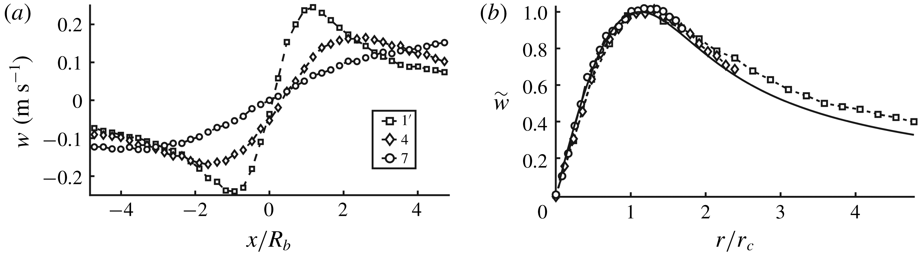
Figure 7(a) shows the local azimuthal velocity
 $w$
in cross-sections
 $1^{\prime }$
, 4, 7 after removal of the transport velocity and azimuthal averaging. The scaling by (3.10) of the profiles clearly indicates the existence of self-similarity of the local azimuthal velocity inside the tip vortex (figure 7
b). These velocity profiles show a slight difference as compared to the non-dimensional self-similarity solutions (3.8) with the Gaussian core reproduced by the data in table 2. This difference is most likely due to wall effects, which generate a swirling flow (Alekseenko et al.
Reference Alekseenko, Kuibin and Okulov2007) that creates an additional vorticity surrounding the original vortex core. The experiments of Quaranta et al. (Reference Quaranta, Bolnot and Leweke2015) revealed large deviations from a Gaussian vortex, which can be explained by wall effects, as the rotor in their experiments was located less than a rotor diameter from the wall.


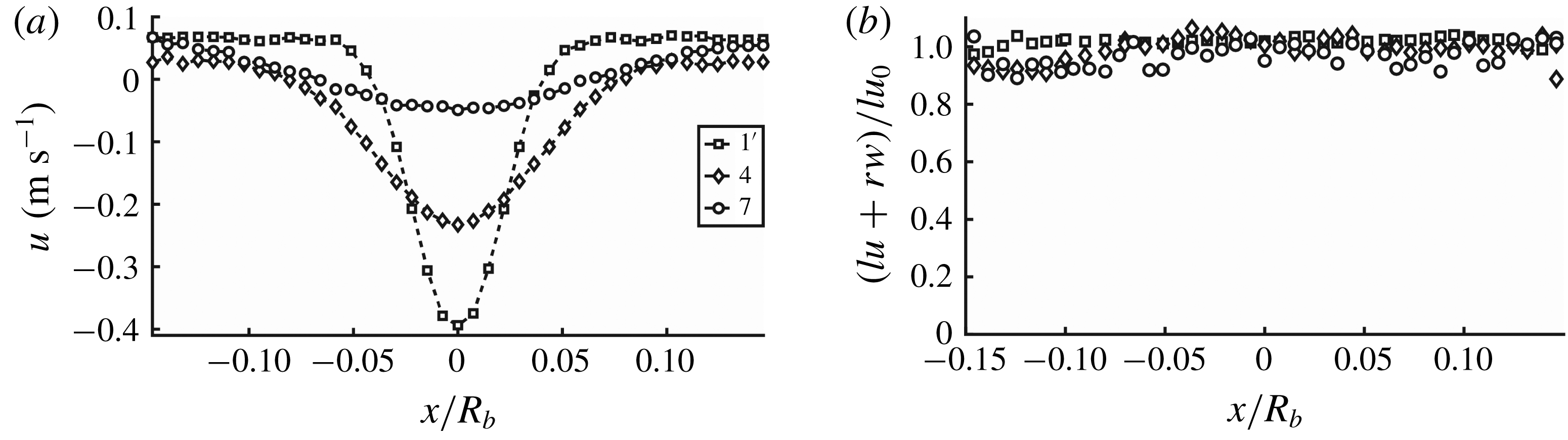
(
 $a$
) Lines with symbols are the original PIV profiles of the local axial velocity in the different cross-sections of the tip vortex. (
 $b$
) Symbols show the correlations between the local azimuthal and axial velocities, using (3.5) to identify the pitch
 $l$
.

Figure 8(a) shows the local axial velocity
 $u$
extracted directly from the global azimuthal velocity
 $W^{\ast }$
. A small total wake rotation exists due to the hub vortex generated in the centre of the rotor wake, which gives rise to a negative overshoot of the local axial velocity profiles (figure 8
a). This, however, vanishes further downstream in the wake. A visual demonstration of the existence of a local axial motion in the centre of the tip vortex was given by Quaranta et al. (Reference Quaranta, Bolnot and Leweke2015) using dye injections in the core of the tip vortex. This axial motion is generated by the local structure of the helical vortex lines of the tip vortices (figure 1
c). However, the existence of an ambient wake rotation with an unknown velocity
 $W^{\ast }(X^{\ast },Y^{\ast },Z^{\ast })$
does not permit a solid conclusion regarding the actual size of the local axial velocity deficit
 $B=W^{\ast }-u_{0}$
. Indeed, only
 $u_{0}=u(x,0)$
can be determined directly from the profiles in figure 8(a). This problem can be avoided if the core of the helical vortex has a local helical structure consisting of local vortex lines (figure 1
c). In this case, the local helical symmetry condition (3.5) between axial and azimuthal velocities can be exploited with an acceptable accuracy, which only depends on measurement errors and disturbances from the surrounding helical vortices (including the turns of the investigated vortex). Furthermore, the linear velocity formulation for local helical symmetry (3.5) allows the usage of averaged velocity fields (3.9) to determine the helical vortex characteristics. The good correlation of the velocity profiles (figure 8
b) in accordance with the formula (3.5) permits one to conclude the existence of a local helical structure of the tip vortex core. Furthermore, it gives the values of the pitch
 $l$
of the local helical symmetry (figure 9(a) and table 2). The relative error of the helical pitch
 $l$
was estimated to be about 10 %.
As a next step, we transform the original local axial velocity profiles (figure 8
a) into the form
 $u_{d}(x,r)=[u(x,r)-u_{0}(x)]$
. In order to assess the similarity of the deficit profiles, the profiles are scaled with
 $\unicode[STIX]{x1D6E4}/2\unicode[STIX]{x03C0}l$
. This result is shown in figure 9(b) where the deficit velocity, made dimensionless by
 $\unicode[STIX]{x1D6E4}/2\unicode[STIX]{x03C0}l$
, depends inversely on the axial distance
 $(1/x)$
, as indicated by the self-similar solution (3.8). The comparisons clearly indicate that the local flow distribution in the tip vortex core is Gaussian and that it exhibits helical self-similarly.


5 Conclusions
Helical tip vortices generated by a three-bladed rotor were measured using stereoscopic PIV measurements in a water flume, with the aim of investigating possible self-similarity of the velocity profiles in the vortex core. The data were analysed and processed assuming different self-similarity scaling arguments. Both the local azimuthal vorticity profiles and the local axial and azimuthal velocity components were investigated and showed the existence of helical self-similarity, which is well described by the proposed model (3.8) and (4.1). Furthermore, a good correlation existed between measurements and vortex flow decay using Batchelor’s vortex ((3.6) and (3.7a,b )) with a Gaussian vortex core. The proposed helical self-similarity scaling arguments enable further investigations of, for example, the stability of helical vortex cores, where expressions of full velocity profiles along the vortex axis are required. The proposed model was developed and tested for flows close to the design operating condition of the wind turbine, where a clearly defined vortex structure is formed. However, at flow conditions where the regular vortex structure is destroyed by external disturbances, or at extreme off-design operating conditions, the validity of the model may be questionable. A study of the limitations of the model will be the subject for future work.
The achieved knowledge is important for the fundamental understanding of vortex flows as well as for different practical applications in which the parametric description requires the use of simplified analytical engineering expressions. Examples of this are tip vortices behind aerodynamic devices, such as vortex generators, and fixed and rotary aircraft, and in combustion chambers and cyclone separators.
Acknowledgement
The research was supported by the RSF (Project no. 14-19-00487).