
 g





1. Introduction
Bell X-1 broke the sound barrier in 1947 with the help of wind-tunnel tests that fell short of fully replicating the Bell X-1 flight environment due to tunnel–wall interference and a lower-than-desired Reynolds number. In 1953, the Douglas D-558-2 Skyrocket became the first aircraft to reach twice the speed of sound without fully knowing the aerodynamic loads a priori from ground test simulation (Griffith et al. Reference Griffith, Maus, Majors and Best1987). With the advent of hypersonic spaceflight, which is characterised by Mach numbers,
 $M \geq 5$
, where dissociation of air begins to become significant and heat loads become high, the ground test facilities proved to be less able to simulate the flight environment, underscoring the persistent gap between ground testing and true flight conditions.
It remains extraordinarily difficult to duplicate the full aerothermochemical environment of the stagnation region in the ground facilities at hypersonic relevant conditions. This difficulty in simultaneously reproducing flight conditions such as Mach number, Reynolds number
 $\textit{Re}$
, shear stress, real gas chemistry and viscous effects in any single ground facility constitutes what can be classically termed the hypersonic simulation problem (Griffith et al. Reference Griffith, Maus, Majors and Best1987). The classical formulation posed the problem mainly in terms of globally averaged aerodynamic loads and the discrepancies between their preflight predictions and the values inferred from flight data. With rapid advances in high-speed flight in recent decades, the modern formulation of this problem targets the same underlying difficulty, now in a regime where complex aerothermochemical effects like dissociation, gas–surface interaction, radiation and material response all play central roles in the stagnation region and boundary layer (BL). The inclusion of additional physical effects introduces additional controlling parameters, making simultaneous matching in a single ground test facility rarely feasible. Consequently, hypersonic research relies on a suite of complementary facilities, spanning high-enthalpy and plasma environments, to isolate specific aspects of the flight physics by matching selected non-dimensional groups (del Val et al. Reference del Val, Chazot and Magin2020). A complete characterisation of real flight conditions thus requires coordinated efforts across both high-enthalpy facilities and plasma wind tunnels (Chazot & Panerai Reference Chazot and Panerai2015; Gu & Olivier Reference Gu and Olivier2020).
In ground-based atmospheric re-entry studies, the primary objective is to reproduce the near-wall environment, namely the shear stresses, the reactive species within the BLand the resulting wall-heat flux. Many such studies focus on the similitude of the key parameters to enable extrapolation from laboratory to flight values, i.e. matching as many non-dimensional parameters as possible. One of the earliest ground-to-flight similarity concepts is binary scaling, which provides a similarity rule for the chemically non-equilibrium inviscid flow over blunt bodies using the Lighthill–Freeman ideal dissociating gas (Freeman Reference Freeman1958). Analysis shows that, in the regime where dissociation dominates recombination, the equations collapse to a single similarity parameter proportional to the product of the edge density and characteristic length,
 $\rho _e L$
. Thus, two flows with the same binary scaling parameter
 $\rho _{\text{e}} L$
have similar non-equilibrium shock-layer and dissociation fields even if their individual density and length differ (Gibson & Marrone Reference Gibson and Marrone1964; Muylaert Reference Muylaert1996; Inger et al. Reference Inger, Higgins and Morgan2003). A second popular method is the concept of local heat transfer simulation (LHTS), proposed by Kolesnikov (Reference Kolesnikov1993, Reference Kolesnikov2000), to reproduce the highest heat load at the stagnation point of the vehicle. The LHTS shows that the stagnation-point heat flux in flight can be reproduced on a test sample in a subsonic facility by matching the centreline free-stream enthalpy, stagnation pressure and velocity gradient between the laboratory case and the hypersonic flight case. In addition, LHTS assumes that local thermal equilibrium and local chemical equilibrium hold at the boundary-layer edge of the test sample.
Traditional extrapolation-to-flight methodologies, as outlined above, are usually formulated for experiments, with simple empirical or semi-analytical justifications; computational fluid dynamics (CFD) and data-assisted extrapolation efforts are presented in von Kaenel et al. (Reference von Kaenel, Sanchi, Vos, Gaffurri, Leyland, Walloschek and Binetti2009), Dreyer et al. (Reference Dreyer, Klock, Grier, McNamara and Cesnik2017) and Fedeli (Reference Fedeli2024). Very few mathematical or analytical efforts have been pursued beyond basic similarity theory to address the extrapolation-to-flight challenge. In this work, we leverage Lie equivalence symmetries to derive new relations that seek to link laboratory-scale observations to their flight-scale counterparts. The present work is inspired by the study of Tranchant et al. (Reference Tranchant, Charpentier, Van Box Som, Ciardi and Falize2022, Reference Tranchant, Charpentier, Van Box Som, Ciardi and Falize2025), in which Lie equivalence transformations are used to analyse extreme astrophysical phenomena in laboratory settings. As opposed to the standard Lie symmetries, Lie equivalence transformations scale not only the independent and dependent variables in the governing equations, but also the underlying property laws. These transformations act on the physical material elements of a model (such as constitutive or transport laws) in addition to the field variables, thereby mapping entire classes of problems into one another. The versatility of these symmetries allows them to be generalised to different systems. The method of Lie-symmetry transformations has been used in many branches of physical sciences to develop particular solutions of differential equations (Ibragimov Reference Ibragimov1994). In fluid dynamics, several studies (Oberlack Reference Oberlack1999, Reference Oberlack2001; Lindgren et al. Reference Lindgren, Österlund and Johansson2004; Oberlack et al. Reference Oberlack, Cabot, Reif and Weller2006; She et al. Reference She, Chen and Hussain2011; Rosteck Reference Rosteck2014) on plane-parallel turbulent shear flows and zero-pressure-gradient turbulent BLs use Lie point symmetries to derive families of invariant scaling laws for mean velocity and higher-order moments.
All of the aforementioned fluid dynamic studies used classical Lie-symmetry methods to derive scaling laws. In this work, we go one step further and, for the first time, demonstrate the applicability of Lie equivalence symmetries in stagnation-point boundary-layer theory to obtain transformations that enable us to go beyond classical similitude. Rather than enforcing classical similitude by matching selected non-dimensional groups, we adopt an equivalence-symmetry viewpoint that identifies invariant symmetry groups of the family of governing equations with arbitrary property laws (arbitrary in the context of equivalence-symmetry analysis means that the property laws are not fixed in the governing equations, and that they are arbitrary functions of one of the field variables). Classical similarity parameters may then emerge as special cases of invariants associated with admitted scaling transformations. This viewpoint is consistent with the standard connection between dimensional analysis and Lie scaling symmetries: for boundary-value problems such as the Prandtl–Blasius BL, invariance under a one-parameter Lie group of scalings can produce the similarity reduction directly, and in this sense scaling symmetry provides a generalisation of dimensional analysis for reducing the number of independent variables (Cantwell Reference Cantwell2002; She et al. Reference She, Chen and Hussain2011). A rich discussion on this can be found in Bluman & Anco (Reference Bluman and Anco2002).
For the ease of implementation and to provide a clear proof of concept, we apply the Lie equivalence framework to the similarity-reduced stagnation-point ordinary differential equations (ODEs) discussed in Bottin (Reference Bottin1999), Barbante et al. (Reference Barbante2001) and Lanza et al. (Reference Lanza, Franco, Elliott, Panesi and Panerai2025). We recognise that the resulting equivalence-symmetry group may be more restrictive than the one that would be obtained for the full stagnation-point partial differential equation (PDE) system. The ODEs are a similarity-reduced form of the same underlying laws, for which the determining equations reduce to a manageable problem while still yielding a meaningful subgroup of the full PDE equivalence and practically usable laboratory–flight mappings.
2. Lie equivalence symmetries of stagnation-point ODEs
In this section, the theoretical results from Lie equivalence-symmetry analysis of the system of stagnation-point ODEs will be presented. For the paper to be self-contained, we have included the detailed derivations of the symmetries and final invariants relevant for mapping in the text below. At this point, we strongly encourage the reader to refer to Appendix A for a brief introduction to the Lie-symmetry/equivalence concepts used in this study. The stagnation-point ODEs as described in Lanza et al. (Reference Lanza, Franco, Elliott, Panesi and Panerai2025) read
 \begin{align} \frac {{\rm d}V}{{\rm d}\eta } &= -F, \\[-10pt] \nonumber \end{align}
 \begin{align} V\frac {{\rm d}F}{{\rm d}\eta } &= \frac {1}{2}\left (R_\rho - F^{2}\right ) + \frac {d}{{\rm d}\eta }\left (\ell _0\frac {{\rm d}F}{{\rm d}\eta }\right ) \!, \\[-10pt] \nonumber \end{align}
 \begin{align} V\frac {{\rm d}g}{{\rm d}\eta } &= \frac {1}{C_{\kern-1pt p}}\frac {d}{{\rm d}\eta }\left (\chi \frac {{\rm d}g}{{\rm d}\eta }\right ) \!, \\[10pt] \nonumber \end{align}
where
 \begin{align} F = \frac {u}{u_e}, \quad g = \frac {T}{T_e}, \quad V = \frac {2\xi }{\partial \xi / \partial x}\left (F \frac {\partial \eta }{\partial x} + \frac {\rho v r}{\sqrt {2\xi }}\right ) \!, \quad R_\rho = \frac {\rho _{\text{e}}}{\rho }, \\[-28pt] \nonumber \end{align}
 \begin{align} \xi (x) = \int _{0}^{x} \rho _e \mu _e u_e r^{2} \, {\rm d}x', \quad \eta (x,y) = \frac {r u_e}{\sqrt {2\xi }} \int _{0}^{y} \rho \, {\rm d}y', \\[-28pt] \nonumber \end{align}
 \begin{align} l_0 = \frac {\rho \mu }{\rho _e \mu _e}, \quad \chi = \frac {\lambda \rho }{\rho _e \mu _e}. \\[-12pt] \nonumber \end{align}
Rewriting (2.1) in the standard form yields
 \begin{align} \Delta _C &:= \frac {{\rm d}V}{{\rm d}\eta } +F =0, \\[-12pt] \nonumber \end{align}
 \begin{align} \Delta _M &:= \frac {d^2F}{{\rm d}\eta ^2} - \frac {1}{\ell _0} \left [ V\frac {{\rm d}F}{{\rm d}\eta } - \frac {1}{2} (R_\rho - F^{2}) -\frac {{\rm d}F}{{\rm d}\eta } \frac {{\rm d}\ell _0}{{\rm d}g} \frac {{\rm d}g}{{\rm d}\eta } \right ]=0, \\[-12pt] \nonumber \end{align}
 \begin{align} \Delta _E &:= \frac {d^2g}{{\rm d}\eta ^2} - \frac {1}{\chi } \left [ C_{\kern-1pt p} V\frac {{\rm d}g}{{\rm d}\eta } - \left ( \frac {{\rm d}g}{{\rm d}\eta } \right )^2 \frac {{\rm d}\chi }{{\rm d}g} \right ]=0. \\[10pt] \nonumber \end{align}
The subscript ‘
 $e$
’ denotes the value of the variable computed at the edge of the BL, where
 $u$
is the velocity,
 $T$
temperature,
 $r$
the radius of the axisymmetric body,
 $\rho$
density,
 $\mu$
dynamic viscosity, and
 $\lambda$
thermal conductivity. For more details about the transformations used to derive the above ODEs from their underlying mass, momentum and energy PDEs, the interested reader is referred to Bottin (Reference Bottin1999), Barbante et al. (Reference Barbante2001) and Lanza et al. (Reference Lanza, Franco, Elliott, Panesi and Panerai2025). It should be emphasised that the standard form of ODEs (2.5) is purely an algebraic rearrangement, introduced only to cast the system into a form that is convenient for Lie equivalence-symmetry analysis. In the equivalence analysis of the stagnation-point ODE system, the set of elements
 $a_i = \{\ell _0, \chi , R_\rho ,C_{\kern-1pt p}\}$
should be regarded as functions of the non-dimensional temperature
 $g$
, with the edge temperature (
 $T_e$
) and pressure (
 $p$
) acting as fixed parameters that identify the particular thermochemical-property table used for a given case. For example,
 $\ell _0(g;T_e,p) = {\rho \mu }/ {(\rho _e \mu _e)} = \rho (gT_e,p) \mu (gT_e,p)/ {(\rho (T_e,p)\mu (T_e,p))}, \,\chi (g;T_e,p) = {\lambda \rho }/ {(\rho _e \mu _e}) = \lambda (gT_e, p)$
 ${\rho (gT_e, p)}/$
 $ (\rho (T_e, p) \mu (T_e,p)).$
Since
 $T_e$
and
 $p$
do not appear explicitly in the ODEs, equivalence symmetries do not transform them directly. Therefore, they do not add any new degrees of freedom to the symmetry, and only act as labels for the property tables from which the elements in
 $a_i$
are built, such that
 $a_i = a_i(g;T_e,p)$
. Unless explicitly stated,
 $T_e$
and
 $p_s$
in the argument of the property laws will be suppressed for brevity and these constitutive functions will be declared as
 $a_i(g)$
. Based on the explicit
 $g$
-dependence of the auxiliary elements
 $a_i$
, the system of auxiliary equations written in the standard form is
 \begin{align} \Delta _{a_{i,k}} := \frac {\partial a_i}{\partial x_k} = 0 , \end{align}
where
 $a_i \in \{R_{\rho },C_{\kern-1pt p},\ell _0,\chi \}$
and
 $x_k \in \{\eta , F, V\}$
. These equations constrain the auxiliary functions
 $a_i$
with respect to
 $\eta ,F, \text{ and } V$
while leaving the
 $g$
-dependence unconstrained.
The infinitesimal generator and its prolongations for the equivalence transformations of the systems of equations (2.5) and (2.6) can be written as
 \begin{align} X &= \phi _{\eta } \partial _{\eta } + \sum ^{\{F,V,g \}}_{{d_i \in }} \phi _{d_i} \partial _{d_i} + \sum _{{a_i \in }}^{\{R_\rho , C_{\kern-1pt p}, \ell _0, \chi \}} \phi _{a_i} \partial _{a_i}, \\[-12pt] \nonumber \end{align}
 \begin{align} X^{(1)} &= X + \sum _{{d_i \in }}^{\{F,V,g \}} \phi ^{(1)}_{d_i} \partial _{{d_i}^{(1)}} + \sum _{{a_i \in }}^{\{R_\rho ,C_{\kern-1pt p},\ell _0,\chi \}} \sum _{{x_j \in }}^{\{\eta ,F,V,g \}} \phi ^{(1)x_j}_{a_i} \partial _{{a_i}^{(x_j)}}, \\[-12pt] \nonumber \end{align}
 \begin{align} X^{(2)} &= X^{(1)} + \sum _{{d_k \in }}^{\{F,g \}} \phi ^{(2)}_{d_k} \partial _{{d_k}^{(2)}}. \\[0pt] \nonumber \end{align}
The superscripts
 $(1)$
and
 $(2)$
on the variables
 $d_{i}$
and
 $d_k$
in
 $X^{(1)}$
and
 $X^{(2)}$
denote their first and second derivatives with respect to
 $\eta$
, respectively, where the variables represented by
 $\phi$
are infinitesimals. The superscript
 $(x_j)$
in equation for
 $X^{(1)}$
denotes the first derivative of the variables collected in
 $a_i$
with respect to the variable
 $x_j$
. The superscripts
 $(1)$
and
 $(2)$
on the
 $\phi$
variables in
 $X^{(1)}$
and
 $X^{(2)}$
are merely indices and do not denote derivatives of
 $\phi$
. Any other index without parentheses is a label. When projecting the universal generator onto a given equation, only a subset of its terms is retained; the remaining terms vanish or are inapplicable for that equation and/or the auxiliary manifold. We restrict to the equivalence group in which the infinitesimals associated with the base variables
 $(\eta ,F,V,g)$
depend only on
 $(\eta ,F,V,g)$
, whereas the infinitesimals for the property laws
 $\boldsymbol{a}=\{\ell _0,\chi ,R_\rho ,C_{\kern-1pt p}\}$
may depend on
 $(\eta ,F,V,g,\boldsymbol{a})$
; which is the standard convention in equivalence-group treatments (e.g. Tranchant et al. Reference Tranchant, Charpentier, Van Box Som, Ciardi and Falize2025).
In the subsequent sections, to obtain the equivalence symmetries, we project the prolonged generator
 $X^{(2)}$
first onto the auxiliary equations (2.6), and subsequently to each equation in the main system (2.5).
2.1. Auxiliary system of equations
Because the auxiliary system of equations contains only first derivatives of the constitutive elements, projecting the second prolongation
 $X^{(2)}$
onto the auxiliary manifold retains only the first-order prolongation terms
 $\phi _{a_i}^{(1)x_j}$
for
 $x_j \in \{\eta ,F,V \}$
.The linearised symmetry condition (LSC) for this system reads,
 $X^{(2)} [\Delta _{A_{i,k}} ] = 0,$
yielding
 \begin{align} \phi _{a_i}^{(1)x_j} = 0, \ \forall \quad a_i \in \{R_\rho ,C_{\kern-1pt p},\ell _0,\chi \} \text{ and } x_j \in \{\eta , F,V\}. \end{align}
For
 $a_i \in \{R_\rho ,C_{\kern-1pt p},\ell _0,\chi \}$
and
 $x_j \in \{\eta ,F,V,g\}$
, we know that
 \begin{align} \phi ^{(1)x_j}_{a_i} = D_{x_j}(\phi _{a_i}) - \sum _{x_m \in }^{\{\eta ,F,V,g\}} a_{i,x_m}\,D_{x_j}\!\left (\phi _{x_m}\right ). \end{align}
Where
 $D$
is the total derivative operator discussed below. To illustrate the structure of this sum, a few representative terms are written out below while keeping
 $a_i$
general
 \begin{align} \text{For } x_k = \eta : \notag \\ \phi ^{(1)\eta }_{a_i} &= D_{\eta }(\phi _{a_i}) - \frac {\partial a_i}{\partial \eta } D_{\eta }(\phi _\eta ) - \frac {\partial a_i}{\partial F} D_{\eta }(\phi _F) - \frac {\partial a_i}{\partial V} D_{\eta }(\phi _V) - \frac {\partial a_i}{\partial g} D_{\eta }(\phi _g). \\[-12pt] \nonumber \end{align}
 \begin{align} \text{For } x_k = F: \notag \\ \phi ^{(1)F}_{a_i} &= D_{F}(\phi _{a_i}) - \frac {\partial a_i}{\partial \eta } D_{F}(\phi _\eta ) - \frac {\partial a_i}{\partial F} D_{F}(\phi _F) - \frac {\partial a_i}{\partial V} D_{F}(\phi _V) - \frac {\partial a_i}{\partial g} D_{F}(\phi _g). \\[-12pt] \nonumber \end{align}
 \begin{align} \text{For } x_k = V: \notag \\ \phi ^{(1)V}_{a_i} &= D_{V}(\phi _{a_i}) - \frac {\partial a_i}{\partial \eta } D_{V}(\phi _\eta ) - \frac {\partial a_i}{\partial F} D_{V}(\phi _F) - \frac {\partial a_i}{\partial V} D_{V}(\phi _V) - \frac {\partial a_i}{\partial g} D_{V}(\phi _g). \\[10pt] \nonumber \end{align}
For any
 $a_i$
, imposing
 $\partial _\eta a_i = \partial _F a_i = \partial _V a_i = 0$
on the auxiliary manifold, only the last term corresponding to
 $x_m=g$
survives in the sum. Therefore, these expressions reduce to
 \begin{align} \phi ^{(1)\eta }_{a_i} &= D_{\eta }(\phi _{a_i}) - \frac {\partial a_i}{\partial g} D_{\eta }(\phi _g), \text{ for } x_k = \eta , \\[-12pt] \nonumber \end{align}
 \begin{align} \phi ^{(1)F}_{a_i} &= D_{F}(\phi _{a_i}) - \frac {\partial a_i}{\partial g} D_{F}(\phi _g), \text{ for } x_k = F , \\[-12pt] \nonumber \end{align}
 \begin{align} \phi ^{(1)V}_{a_i} &= D_{V}(\phi _{a_i}) - \frac {\partial a_i}{\partial g} D_{V}(\phi _g), \text{ for } x_k = V . \\[10pt] \nonumber \end{align}
Given that the infinitesimals
 $\phi _{a_i} \text{ and } \phi _g$
are functions of only the base variables and arbitrary properties, their total derivatives with respect to base variables do not contain the arbitrary gradient
 $\partial a_i/\partial g$
. Therefore a relation of the form
 $P(\eta ,F,V,g, a_i) - ({\partial a_i}/{\partial g})\,Q(\eta ,F,V,g,a_i) = 0$
must hold for all admissible
 $a_i$
only if
 $P(\eta ,F,V,g, a_i) = 0, Q(\eta ,F,V,g, a_i) = 0.$
Applying this argument to the expressions (2.11) above yields
 \begin{align} D_\eta (\phi _{a_i}) &= D_F(\phi _{a_i}) = D_V(\phi _{a_i}) = 0, \\[-12pt] \nonumber \end{align}
 \begin{align} D_\eta (\phi _g) &= D_F(\phi _g) = D_V(\phi _g)=0. \\[10pt] \nonumber \end{align}
In the auxiliary equations, only
 $a_i$
enters the system as a dependent variable, the rest of the variables
 $x_k\in \{\eta ,F,V,g\}$
are regarded as independent coordinates, so there are no jet variables such as
 $\partial _\eta F$
,
 $\partial _\eta V$
,
 $\partial _V \eta$
,
 $\partial _F V$
and so on. Consequently the total derivatives become
 \begin{align} D_\eta = \frac {\partial }{\partial \eta } + \sum _{a_i}\frac {\partial a_i}{\partial \eta } \frac {\partial }{\partial a_i}, \ \ D_V = \frac {\partial }{\partial V} + \sum _{a_i}\frac {\partial a_i}{\partial V} \frac {\partial }{\partial a_i}, \ \ D_F = \frac {\partial }{\partial F} + \sum _{a_i}\frac {\partial a_i}{\partial F} \frac {\partial }{\partial a_i}. \end{align}
Imposing the auxiliary constraints
 $\partial _\eta a_{i}= \partial _F a_{i}= \partial _V a_{i}=0$
reduces these total derivatives, when acting on the infinitesimals
 $\phi _g$
and
 $\phi _{a_i}$
, to
 \begin{align} D_\eta = \frac {\partial }{\partial \eta },\qquad D_F = \frac {\partial }{\partial F},\qquad D_V = \frac {\partial }{\partial V}. \end{align}
Using the above in the determining equations (2.12), we get
 \begin{align} {\phi _g = \phi _g(g),} \qquad {\phi _{a_i} = \phi _{a_i}(g,R_\rho ,\ell _0,C_{\kern-1pt p},\chi ).} \end{align}
2.2. Continuity equation
The LSC for (2.5a ) is
 \begin{align} X^{(2)}[\Delta _C] = 0. \end{align}
The continuity equation is a first-order ODE, therefore the coefficients up to first order in
 $X^{(2)}$
enter the LSC, and the second-order prolongation terms vanish identically. Additionally, the terms corresponding to arbitrary functions also drop out for this case. From (2.16), we have
 \begin{align} \phi ^{(1)}_V + \phi _F = 0 . \end{align}
Substituting
 $\phi ^{(1)}_V=D_{\eta }(\phi _V)-V^{(1)}D_{\eta }(\phi _{\eta })$
and expanding the total derivative
 $D_\eta = \partial _\eta + F^{(1)}\partial _F + V^{(1)}\partial _V + g^{(1)}\partial _g$
, we obtain
 \begin{align} \partial _\eta \phi _V + F^{(1)} \partial _F \phi _V + V^{(1)} \partial _V \phi _V + g^{(1)} \partial _g \phi _V - V^{(1)}\bigl ( \partial _\eta \phi _\eta + F^{(1)} \partial _F \phi _\eta \nonumber \\[4pt]\quad + V^{(1)} \partial _V \phi _\eta + g^{(1)} \partial _g \phi _\eta \bigr ) + \phi _F=0 . \end{align}
Using
 $V^{(1)}=-F$
, collecting the coefficients of the independent jet variables, and grouping the remaining zeroth-order terms, results in
 \begin{align} F^{(1)}\bigl (\partial _F \phi _V + F \partial _F \phi _\eta \bigr ) + g^{(1)}\bigl (\partial _g \phi _V + F \partial _g \phi _\eta \bigr ) + F\bigl (-\partial _V \phi _V + \partial _\eta \phi _\eta \bigr ) \nonumber \\[4pt]\quad - F^2 \partial _V \phi _\eta + \partial _\eta \phi _V + \phi _F = 0. \end{align}
The aforementioned convention on superscripts applies here and throughout the main article. For example,
 $F^{(1)}:=\partial F/\partial \eta$
etc.
Splitting on
 $F^{(1)}, g^{(1)}$
and the remaining zero-order terms, we get the determining equations for the equivalence-symmetry analysis of the continuity equation as
 \begin{align} \partial _F \phi _V + F \partial _F \phi _\eta &= 0, \\[-10pt] \nonumber \end{align}
 \begin{align} \partial _g \phi _V + F \partial _g \phi _\eta &= 0, \\[-10pt] \nonumber \end{align}
 \begin{align} F\bigl (-\partial _V \phi _V + \partial _\eta \phi _\eta \bigr ) - F^2 \partial _V \phi _\eta + \partial _\eta \phi _V + \phi _F &= 0. \\[10pt] \nonumber \end{align}
To solve the above system to derive meaningful dependencies, we assume the spatial coordinate transformation does not depend on the velocities or temperature, implying
 $\phi _\eta = \phi _\eta (\eta )$
, which readily yields
 \begin{align} \left . \begin{aligned} \partial _F \phi _V &= 0, \\[4pt]\partial _F \phi _\eta &= 0, \end{aligned} \right \} &\quad \text{from} (2.20a) , \\[-12pt] \nonumber \end{align}
 \begin{align} \left . \begin{aligned} \partial _g \phi _V &= 0, \\[4pt]\partial _g \phi _\eta &= 0, \end{aligned} \right \} &\quad \text{from} (2.20b) . \\[10pt] \nonumber \end{align}
The first of both equations (2.21a ) and (2.21b ) give
 \begin{align} \phi _V = \phi _V(\eta , V) . \end{align}
Now using the above together with
 $\phi _\eta = \phi _\eta (\eta )$
in the zero-order split, we get
 \begin{align} \phi _F= F \left ( \partial _V \phi _V - \partial _\eta \phi _\eta \right )-\partial _\eta \phi _V . \end{align}
2.3. Momentum equation
In this section, the prolonged infinitesimal generator (2.7c ) is projected onto the momentum equation (2.5b ) to yield the LSC as
 \begin{align} X^{(2)}[\Delta _M] = 0 . \end{align}
Since (2.5b
) contains the second-order derivative of
 $F$
and first-order derivatives of
 $F \text{ and } g$
with respect to
 $\eta$
, and of
 $\ell _0$
with respect to
 $g$
, the prolongations corresponding to these terms will be non-zero. The reduced LSC (2.24) yields
 \begin{align} \phi _F^{(2)} ={}& \big ( \phi _\eta \partial _\eta +\phi _V \partial _V + \phi _F \partial _F + \phi _g \partial _g + \phi _{\ell _0} \partial _{\ell _0} + \phi _{R_\rho } \partial _{R_\rho } \notag \\[5pt]& + \phi ^{(1)}_F \partial _{F^{(1)}} + \phi ^{(1)}_g \partial _{g^{(1)}} + \phi ^{(1)g}_{\ell _0} \partial _{\ell _0^{(g)}} \big ) \mathbb{M}, \end{align}
where the following shorthand has been adopted:
 \begin{align} \mathbb{M}=\frac {1}{l_0} \left [ V\frac {{\rm d}F}{{\rm d}\eta } - \frac {1}{2} (R_\rho - F^{2}) -\frac {{\rm d}F}{{\rm d}\eta } \frac {{\rm d}l_0}{{\rm d}g} \frac {{\rm d}g}{{\rm d}\eta } \right ] \! . \end{align}
Before we expand (2.25), the prolonged infinitesimals
 $\phi _g^{(1)}, \phi _F^{(1)}, \phi ^{(1)g}_{\ell _0}$
and
 $\phi _F^{(2)}$
can be obtained as follows:
 \begin{align} \phi _g^{(1)} &= D_\eta \big ( \phi _g \big ) - \frac {{\rm d}g}{{\rm d}\eta } D_\eta \big ( \phi _\eta \big ) , \\[-10pt] \nonumber \end{align}
 \begin{align} \phi _F^{(1)} &= D_\eta \big ( \phi _F \big ) - \frac {{\rm d}F}{{\rm d}\eta } D_\eta \big ( \phi _\eta \big ) , \\[-10pt] \nonumber \end{align}
 \begin{align} \phi _F^{(2)} &= D_\eta \big ( \phi ^{(1)}_F \big ) - \frac {d^2 F}{{\rm d}\eta ^2} D_\eta \big ( \phi _\eta \big ) . \\[10pt] \nonumber \end{align}
Using
 $D_\eta = \partial _\eta +({\rm d}F/{\rm d}\eta )\partial _F +({\rm d}V/{\rm d}\eta )\partial _V + ({\rm d}g/{\rm d}\eta )\partial _g + d^2F/{\rm d}\eta ^2 \partial _{F^{(1)}} + d^2g/ {\rm d}\eta ^2 \partial _{g^{(1)}} + \ldots$
together with
 $\phi _g=\phi _g(g)$
from (2.15),
 $\phi _\eta =\phi _\eta (\eta )$
and
 $\phi _F$
from (2.23), we get
 \begin{align} \phi _g^{(1)} &= \left ( \frac {d}{{\rm d}g} \big ( \phi _g(g) \big ) - \frac {d}{{\rm d}\eta } \big ( \phi _\eta (\eta ) \big ) \right ) \frac {{\rm d}g}{{\rm d}\eta }, \\[-12pt] \nonumber \end{align}
 \begin{align} \phi _F^{(1)} & = -F^2 \partial _{VV} \phi _V \kern-1pt - \kern-1pt F \frac {d^2}{{\rm d}\eta ^2}\big (\phi _\eta (\eta )\big ) \kern-1pt + \kern-1pt 2F\partial _{V\eta }\phi _V \kern-1pt + \kern-1pt \frac {{\rm d}F}{{\rm d} \eta }\partial _V \phi _V \kern-1pt - \kern-1pt 2 \frac {{\rm d}F}{{\rm d}\eta } \frac {d}{{\rm d}\eta } \big ( \phi _\eta (\eta ) \big ) \kern-1pt - \kern-1pt \partial _{\eta \eta } \phi _V , \\[-12pt] \nonumber \end{align}
 \begin{align} \phi _F^{(2)} &= \mathbb{M} \left ( \partial _V \phi _V - 3\frac {d}{{\rm d}\eta } \big ( \phi _\eta (\eta ) \big ) \right ) -3 F \frac {{\rm d}F}{{\rm d}\eta }\partial _{VV}\phi _V + 3 \frac {{\rm d}F}{{\rm d}\eta }\partial _{\eta V}\phi _V - 3 \frac {{\rm d}F}{{\rm d}\eta } \frac {d^2\big ( \phi _\eta (\eta ) \big )}{{\rm d}\eta ^2} \notag \\ &\quad {} + F^3\partial _{VVV}\phi _V - 3F^2 \partial _{\eta V V} \phi _V - F\frac {d^3\big ( \phi _\eta (\eta ) \big )}{{\rm d}\eta ^3} + 3F\partial _{\eta \eta V} \phi _V - \partial _{\eta \eta \eta } \phi _V. \\[10pt] \nonumber \end{align}
Evaluating the differentials on the right-hand side of (2.25) termwise, we obtain
 \begin{align} \left . \begin{aligned} \partial _\eta \mathbb{M} &= 0, \; \partial _V \mathbb{M} = \frac {1}{\ell _0} \frac {{\rm d}F}{{\rm d}\eta }, \; \partial _F \mathbb{M} = \frac {F}{\ell _0}, \; \partial _g \mathbb{M} = 0, \; \partial _{\ell _0} \mathbb{M} = -\frac {1}{\ell _0} \frac {d^{2}F}{{\rm d}\eta ^{2}}, \; \partial _{R_\rho } \mathbb{M} = -\frac {1}{2\ell _0}, \\[0.3em] \partial _{F^{(1)}} \mathbb{M} &= \frac {1}{\ell _0}\!\left ( V - \frac {{\rm d}\ell _0}{{\rm d}g} \frac {{\rm d}g}{{\rm d}\eta } \right ), \; \partial _{g^{(1)}} \mathbb{M} = -\frac {1}{\ell _0}\!\left ( \frac {{\rm d}\ell _0}{{\rm d}g} \frac {{\rm d}F}{{\rm d}\eta } \right ), \; \partial _{\ell _0^{(g)}} \mathbb{M} = -\frac {1}{\ell _0} \frac {{\rm d}g}{{\rm d}\eta } \frac {{\rm d}F}{{\rm d}\eta } .\end{aligned} \right \} \end{align}
Substituting (2.28) and (2.29) in (2.25), and rearranging, we finally obtain the expanded LSC
 \begin{align} &\frac {{\rm d}F}{{\rm d}\eta }\frac {{\rm d}g}{{\rm d}\eta } \left [ -\frac {1}{\ell _0}\frac {{\rm d}\ell _0}{{\rm d}g}\phi _{\ell _0} + \phi _{\ell _0}^{(1)g} + \frac {{\rm d}\ell _0}{{\rm d}g}\frac {d}{{\rm d}g}\big (\phi _g(g)\big ) \right ] \notag \\[4pt]&\quad + \frac {{\rm d}F}{{\rm d}\eta } \left [ -\phi _V + 3\ell _0 \partial _{\eta V}\phi _V - 3\ell _0 F \partial _{VV}\phi _V - 3\ell _0 \frac {d^2}{{\rm d}\eta ^2}\big (\phi _\eta (\eta )\big ) - V\frac {d}{{\rm d}\eta }\big (\phi _\eta (\eta )\big ) + \frac {\phi _{\ell _0}}{\ell _0}V \right ] \notag \\[4pt]&\quad + \frac {{\rm d}g}{{\rm d}\eta } \left [ -\frac {{\rm d}\ell _0}{{\rm d}g} \left ( \partial _{\eta \eta }\phi _V - 2F\partial _{\eta V}\phi _V + F^2\partial _{VV}\phi _V + F\frac {d^2}{{\rm d}\eta ^2}\big (\phi _\eta (\eta )\big ) \right ) \right ] \notag \\[4pt]&\quad + \left [ -\ell _0\partial _{\eta \eta \eta }\phi _V + F\partial _\eta \phi _V + 3\ell _0 F\partial _{\eta \eta V}\phi _V - \frac {1}{2}F^2\partial _V\phi _V - 3\ell _0 F^2\partial _{\eta VV}\phi _V \right . \notag \\[4pt]&\qquad \qquad + \ell _0 F^3\partial _{VVV}\phi _V - \frac {1}{2}F^2\frac {d}{{\rm d}\eta }\big (\phi _\eta (\eta )\big ) - \ell _0 F\frac {d^3}{{\rm d}\eta ^3}\big (\phi _\eta (\eta )\big ) \notag \\[4pt]&\qquad \qquad + \frac {F^2}{2\ell _0}\phi _{\ell _0} + \frac {1}{2}\phi _{R_\rho } - \frac {1}{2}R_\rho \partial _V\phi _V + \frac {3}{2}R_\rho \frac {d}{{\rm d}\eta }\big (\phi _\eta (\eta )\big ) \notag \\[4pt]&\qquad \qquad \left . - \frac {R_\rho }{2\ell _0}\phi _{\ell _0} + V\partial _{\eta \eta }\phi _V - 2FV\partial _{\eta V}\phi _V + F^2V\partial _{VV}\phi _V + FV\frac {d^2}{{\rm d}\eta ^2}\big (\phi _\eta (\eta )\big ) \right ] =0. \end{align}
We have eliminated the highest derivative by substituting
 $F_{\eta \eta }=\mathbb{M}$
in (2.30). The first derivatives
 ${\rm d}F/{\rm d}\eta$
and
 ${\rm d}g/{\rm d}\eta$
are independent jet coordinates. Therefore, the coefficients of the independent monomials
 $({{\rm d}F}/{{\rm d}\eta })( {{\rm d}g}/{{\rm d}\eta }), {{\rm d}F}/{{\rm d}\eta }, {{\rm d}g}/{{\rm d}\eta }$
and the remaining constant terms must vanish separately. This gives the following determining equations:
 \begin{align} &\text{ coeff. of }\frac {{\rm d}F}{{\rm d}\eta }\frac {{\rm d}g}{{\rm d}\eta }: \notag \\ &-\frac {1}{\ell _0}\frac {{\rm d}\ell _0}{{\rm d}g}\phi _{\ell _0} + \phi _{\ell _0}^{(1)g} + \frac {{\rm d}\ell _0}{{\rm d}g} \frac {d}{{\rm d}g}\big (\phi _g(g)\big ) =0, \\[-12pt] \nonumber \end{align}
 \begin{align} &\text{ coeff. of }\frac {{\rm d}F}{{\rm d}\eta }: \notag \\ &-\phi _V +3\ell _0\partial _{\eta V}\phi _V -3\ell _0F\partial _{VV}\phi _V -3\ell _0\frac {d^2}{{\rm d}\eta ^2}\big (\phi _\eta (\eta )\big ) -V\frac {d}{{\rm d}\eta }\big (\phi _\eta (\eta )\big ) +\frac {\phi _{\ell _0}}{\ell _0}V =0, \\[-12pt] \nonumber \end{align}
 \begin{align} &\text{ coeff. of }\frac {{\rm d}g}{{\rm d}\eta }: \notag \\ &-\frac {{\rm d}\ell _0}{{\rm d}g} \left ( \partial _{\eta \eta }\phi _V -2F\partial _{\eta V}\phi _V +F^2\partial _{VV}\phi _V +F\frac {d^2}{{\rm d}\eta ^2}\big (\phi _\eta (\eta )\big ) \right ) =0, \\[-12pt] \nonumber \end{align}
 \begin{align} &\text{ remaining zero-order terms}: \notag \\[3pt]&-\ell _0\partial _{\eta \eta \eta }\phi _V +F\partial _\eta \phi _V +3\ell _0F\partial _{\eta \eta V}\phi _V -\frac {1}{2}F^2\partial _V\phi _V -3\ell _0F^2\partial _{\eta VV}\phi _V +\ell _0F^3\partial _{VVV}\phi _V \notag \\[3pt]&\quad -\frac {1}{2}F^2\frac {d}{{\rm d}\eta }\big (\phi _\eta (\eta )\big ) -\ell _0F\frac {d^3}{{\rm d}\eta ^3}\big (\phi _\eta (\eta )\big ) +\frac {F^2}{2\ell _0}\phi _{\ell _0} +\frac {1}{2}\phi _{R_\rho } -\frac {1}{2}R_\rho \partial _V\phi _V \notag \\[3pt]&\quad +\frac {3}{2}R_\rho \frac {d}{{\rm d}\eta }\big (\phi _\eta (\eta )\big ) -\frac {R_\rho }{2\ell _0}\phi _{\ell _0} +V\partial _{\eta \eta }\phi _V -2FV\partial _{\eta V}\phi _V +F^2V\partial _{VV}\phi _V \notag \\[3pt]&\quad + FV\frac {d^2}{d\eta ^2}\big (\phi _\eta (\eta )\big ) =0. \\[10pt] \nonumber \end{align}
We now solve these determining equations one by one. Equation (2.31) yields
 \begin{align} \phi ^{(1)g}_{\ell _0} = \left ( \frac {\phi _{\ell _0}}{\ell _0} - \frac {d}{{\rm d}g}\big ( \phi _g(g) \big ) \right ) \frac {{\rm d}\ell _0}{{\rm d}g}. \end{align}
Splitting (2.32) by
 $F$
, we obtain
 \begin{align} 3\ell _0 \partial _{VV}\phi _V = 0 \Rightarrow \phi _V = \mathcal{A}(\eta )V+ \mathcal{B}(\eta ), \end{align}
which immediately gives
 $\partial _{\eta V}\phi _V = \partial _\eta \mathcal{A}(\eta )$
. Using these in (2.32), we get
 \begin{align} -(\mathcal{A}(\eta )V+\mathcal{B}(\eta )) + 3 \ell _0 \frac {{\rm d}\mathcal{A}(\eta )}{{\rm d} \eta } - 3 \ell _0 \frac {d^2}{{\rm d} \eta ^2} \big ( \phi _\eta (\eta ) \big ) - V \frac {d}{{\rm d} \eta } \big ( \phi _\eta (\eta ) \big ) + {V}\frac {\phi _{\ell _0}}{\ell _0} =0 . \end{align}
Splitting by the powers of
 $V$
we get two equations, one for
 $V^1$
and the other for
 $V^0$
, respectively, as,
 \begin{align} &\phi _{\ell _0} = \left ( \mathcal{A}(\eta ) + \frac {d}{{\rm d} \eta } \big ( \phi _\eta (\eta ) \big ) \right ) \ell _0, \\[-12pt] \nonumber \end{align}
 \begin{align} -&\mathcal{B}(\eta ) + 3\ell _0 \left ( \frac {{\rm d}\mathcal{A}(\eta )}{{\rm d} \eta } - \frac {d^2}{{\rm d} \eta ^2} \big ( \phi _\eta (\eta ) \big ) \right )=0 \Rightarrow \mathcal{B}(\eta ) = 0, \text{ and } \frac {{\rm d}\mathcal{A}(\eta )}{{\rm d} \eta } = \frac {d^2}{{\rm d} \eta ^2} \big ( \phi _\eta (\eta ) \big ) \\[10pt] \nonumber \end{align}
Similarly, splitting (2.33) by the powers of
 $F$
, and skipping the intermediate steps for brevity, we obtain
 \begin{align} \partial _{VV}\phi _V &= 0, \text{ for the coeff. of } F^2 , \\[-12pt] \nonumber \end{align}
 \begin{align} \frac {d^2}{{\rm d} \eta ^2} \big ( \phi _\eta (\eta ) \big ) &= 2 \partial _{\eta V}\phi _V, \text{ for the coeff. of } F^1 , \\[-12pt] \nonumber \end{align}
 \begin{align} \partial _{\eta \eta } \phi _V &= 0, \text{ for the coeff. of } F^0 . \\[10pt] \nonumber \end{align}
Using
 $\mathcal{B}(\eta )=0$
from (2.38b
) in (2.36), we get
 $\phi _V = \mathcal{A}(\eta ) V$
, which leads to
 $\partial _{\eta V} \phi _V = {\rm d}\mathcal{A}(\eta )/{\rm d}\eta$
. With this and (2.39b
), we get
 \begin{align} \frac {d^2}{{\rm d} \eta ^2} \big ( \phi _\eta (\eta ) \big ) = 2 \frac {{\rm d}\mathcal A(\eta )}{{\rm d}\eta } . \end{align}
The above equation and the last of (2.38b ) are satisfied only when
 \begin{align} \frac {{\rm d}\mathcal{A}(\eta )}{{\rm d}\eta } = 0 \Rightarrow \mathcal{A}(\eta ) = A_0, \text{a constant} , \end{align}
which immediately yields
 \begin{align} &\frac {d^2}{{\rm d} \eta ^2} \big ( \phi _\eta (\eta ) \big ) = 0 \Rightarrow \frac {d}{{\rm d} \eta } \big ( \phi _\eta (\eta ) \big ) = C_0, \end{align}
where
 $C_0$
is a constant, such that
 \begin{align} & \phi _\eta = C_0 \eta , \end{align}
where the constant of integration is chosen to be zero to preserve the transformed wall coordinate at
 $\hat \eta = 0$
.
Substituting the results obtained so far in (2.34) and (2.23), we obtain
 \begin{align} \phi _{R_\rho } &= 2(A_0-C_0)R_\rho , \\[-10pt] \nonumber \end{align}
 \begin{align} \phi _F &= (A_0 - C_0) F, \\[10pt] \nonumber \end{align}
respectively.
The infinitesimals generated so far by the preceding analysis are
 \begin{align} \left . \begin{aligned} \phi _\eta = C_0 \eta , \quad &\phi _V = A_0 V, \quad \phi _F = (A_0 - C_0) F, \quad \phi _g = \phi _g(g),\\[5pt]&\phi _{R_\rho } = 2(A_0-C_0)R_\rho , \quad \phi _{\ell _0} = (A_0 + C_0 )\ell _0. \end{aligned} \right \} \end{align}
2.4. Energy equation
Following the same procedure as above, the prolonged infinitesimal generator (2.7c ) is projected onto (2.5c ) to yield the LSC for the energy equation as
 \begin{align} X^{(2)}[\Delta _E] = 0 . \end{align}
The energy equation (2.5c
) contains the first- and second-order derivatives of
 $g$
with respect to
 $\eta$
, and the first-order derivative of
 $\chi$
with respect to
 $g$
. Therefore, the prolongations corresponding to these terms will be non-zero. The reduced form of the LSC (2.47) reads
 \begin{align} \phi _g^{(2)} ={}& \big ( \phi _\eta \partial _\eta +\phi _V \partial _V + \phi _g \partial _g + \phi _{\chi } \partial _{\chi } + \phi _{C_{\kern-1pt p}} \partial _{C_{\kern-1pt p}} + \phi ^{(1)}_g \partial _{g^{(1)}} + \phi ^{(1)g}_{\chi } \partial _{\chi ^{(g)}} \big ) \mathbb{E}, \end{align}
where the following shorthand has been adopted:
 \begin{align} \mathbb{E}=\frac {1}{\chi } \left [ C_{\kern-1pt p} V\frac {{\rm d}g}{{\rm d}\eta } - \left ( \frac {{\rm d}g}{{\rm d}\eta } \right )^2 \frac {{\rm d}\chi }{{\rm d}g} \right ] \!. \end{align}
From (2.28a
) and (2.46), the first prolongation
 $\phi ^{(1)}_g = ({{\rm d}\phi _g(g)}/{{\rm d}g} -C_0){\rm d}g/{\rm d}\eta$
. Using this, we obtain the second prolongation
 $\phi ^{(2)}_g$
recursively as
 \begin{align} \phi ^{(2)}_g &= D_\eta \big (\phi ^{(1)}_g \big ) - \frac {d^2g}{{\rm d}\eta ^2} D_\eta \big ( \phi _\eta \big ) \notag \\[4pt]\Rightarrow \phi ^{(2)}_g &= \left ( \frac {{\rm d}g}{{\rm d}\eta } \right )^2 \frac {d^2 }{{\rm d}g^2}\big ( \phi _g(g) \big ) + \left ( \frac {{\rm d}\phi _g(g)}{{\rm d}g} -2C_0 \right ) \frac {d^2g}{{\rm d}\eta ^2} .\end{align}
Evaluating the differentials on the right-hand side of (2.48) termwise, we obtain
 \begin{align} \left . \begin{aligned} \partial _\eta \mathbb{E} &= 0, \; \; \partial _V \mathbb{E} = C_{\kern-1pt p}\frac {1}{\chi } \frac {{\rm d}g}{{\rm d}\eta }, \; \; \partial _g \mathbb{E} = 0, \; \partial _{\chi } \mathbb{E} = -\frac {1}{\chi } \frac {d^{2}g}{{\rm d}\eta ^{2}}, \; \\[0.3em] \partial _{C_{\kern-1pt p}} \mathbb{E} &= \frac {1}{\chi }V\frac {{\rm d}g}{{\rm d}\eta }, \; \; \partial _{g^{(1)}} \mathbb{E} = \frac {1}{\chi }\!\left ( C_{\kern-1pt p} V - 2 \frac {{\rm d}\chi }{{\rm d}g} \frac {{\rm d}g}{{\rm d}\eta } \right ), \; \; \partial _{\chi ^{(g)}} \mathbb{E} = -\frac {1}{\chi } \left ( \frac {{\rm d}g}{{\rm d}\eta } \right )^2 .\end{aligned} \right \} \end{align}
Using
 $\phi ^{(1)}_g, \phi ^{(2)}_g$
and (2.51) in (2.48), and upon simplifying and rearranging, we finally obtain the expanded LSC
 \begin{align} &V\frac {{\rm d}g}{{\rm d}\eta } \left [ -(A_0 + C_0)C_{\kern-1pt p} + C_{\kern-1pt p} \frac {\phi _\chi }{\chi } -\phi _{C_{\kern-1pt p}} \right ] \notag \\ &\quad + \left (\frac {{\rm d}g}{{\rm d}\eta }\right )^2 \left [ \chi \frac {d^2}{{\rm d}g^2}\big (\phi _g(g)\big ) + \frac {{\rm d}\chi }{{\rm d}g}\frac {d}{{\rm d}g}\big (\phi _g(g)\big ) + \phi ^{(1)g}_\chi - \frac {{\rm d}\chi }{{\rm d}g}\frac {\phi _\chi }{\chi } \right ] =0 . \end{align}
Splitting the above equation with respect to the independent monomials
 $V{\rm d}g/{\rm d}\eta$
and
 $({\rm d}g/{\rm d}\eta )^2$
, we obtain the following, respectively:
 \begin{align} \phi _{C_{\kern-1pt p}} &= \left ( -(A_0 + C_0) + \frac {\phi _\chi }{\chi } \right )C_{\kern-1pt p} , \\[-12pt] \nonumber \end{align}
 \begin{align} \chi \frac {d^2}{{\rm d}g^2} \big ( \phi _g(g) \big ) &= \frac {\phi _\chi }{\chi } \frac {{\rm d}\chi }{{\rm d}g} - \phi ^{(1)g}_\chi - \frac {{\rm d}\chi }{{\rm d}g} \frac {d}{{\rm d}g} \big (\phi _g(g) \big ) . \\[10pt] \nonumber \end{align}
Using
 $\phi ^{(1)g}_{\chi } = D_g ( \phi _\chi )- ({\rm d}\chi /{\rm d}g)D_g ( \phi _g (g) ) = D_g ( \phi _\chi )- ({\rm d}\chi /{\rm d}g)({\rm d}\phi _g(g)/{\rm d}g)$
in the second equation above yields
 \begin{align} \chi \frac {d^2}{{\rm d}g^2} \big ( \phi _g(g) \big )= \frac {\phi _\chi }{\chi } \frac {{\rm d}\chi }{{\rm d}g} -D_g \big (\phi _\chi \big ) . \end{align}
Equations (2.53) and (2.55) must hold for all admissible
 $C_{\kern-1pt p}(g)$
and
 $\chi (g)$
. Recall, from (2.15), we have established that
 $\phi _{\chi } = \phi _{\chi }(g,R_\rho ,\ell _0,C_{\kern-1pt p},\chi )$
, therefore we can expand
 $D_g$
as
 \begin{align} D_g(\phi _\chi ) = \frac {\partial \phi _\chi }{\partial _g} + \frac {\partial R_\rho }{\partial g} \frac {\partial \phi _\chi }{\partial R_\rho } + \frac {\partial \ell _0}{\partial g} \frac {\partial \phi _\chi }{\partial \ell _0} + \frac {\partial C_{\kern-1pt p}}{\partial g} \frac {\partial \phi _\chi }{\partial C_{\kern-1pt p}} + \frac {\partial \chi }{\partial g} \frac {\partial \phi _\chi }{\partial \chi } . \end{align}
Substituting this into (2.55) gives
 \begin{align} \chi \,\frac {d^{2}}{{\rm d}g^{2}}(\phi _{g}(g)) = \frac {{\rm d}\chi }{{\rm d}g} \left ( \frac {\phi _{\chi }}{\chi } - \frac {\partial \phi _{\chi }}{\partial \chi } \right ) - \frac {\partial \phi _{\chi }}{\partial g} - \frac {{\rm d}R_{\rho }}{{\rm d}g}\,\frac {\partial \phi _{\chi }}{\partial R_{\rho }} - \frac {{\rm d}\ell _{0}}{{\rm d}g}\,\frac {\partial \phi _{\chi }}{\partial \ell _{0}} - \frac {{\rm d}C_{p}}{{\rm d}g}\,\frac {\partial \phi _{\chi }}{\partial C_{p}}. \end{align}
Since
 $R_\rho (g), \ell _0(g), C_{\kern-1pt p}(g)$
and
 $\chi (g)$
are arbitrary elements of the equivalence class, their first derivatives with respect to
 $g$
are treated as independent auxiliary jet variables. Therefore, the above identity must hold for arbitrary values of
 ${{\rm d}R_{\rho }}/{{\rm d}g},{{\rm d}\ell _{0}}/{{\rm d}g}, {{\rm d}C_{p}}/{{\rm d}g} \text{ and } {{\rm d}\chi }/{{\rm d}g}$
and the coefficients multiplying these independent quantities are split and set to zero separately, together with the remaining derivative-free part
 \begin{align} \text{coefficient of } \frac {{\rm d}R_{\rho }}{{\rm d}g} \qquad &\Rightarrow \qquad \frac {\partial \phi _{\chi }}{\partial R_{\rho }}=0, \\[-12pt] \nonumber \end{align}
 \begin{align} \text{coefficient of } \frac {{\rm d}\ell _{0}}{{\rm d}g} \qquad &\Rightarrow \qquad \frac {\partial \phi _{\chi }}{\partial \ell _{0}}=0, \\[-12pt] \nonumber \end{align}
 \begin{align} \text{coefficient of } \frac {{\rm d}C_{p}}{{\rm d}g} \qquad &\Rightarrow \qquad \frac {\partial \phi _{\chi }}{\partial C_{p}}=0, \\[-12pt] \nonumber \end{align}
 \begin{align} \text{coefficient of } \frac {{\rm d}\chi }{{\rm d}g} \qquad &\Rightarrow \qquad \frac {\phi _{\chi }}{\chi } - \frac {\partial \phi _{\chi }}{\partial \chi }=0, \\[-12pt] \nonumber \end{align}
 \begin{align} \text{remaining terms, } \chi \,\frac {d^{2}}{{\rm d}g^{2}}(\phi _{g}(g)) &= -\frac {\partial \phi _{\chi }}{\partial g} . \\[10pt] \nonumber \end{align}
Equation (2.58d ) has general solution
 \begin{align} \phi _\chi =f(g)\chi , \end{align}
where
 $f(g)$
represents a
 $g$
-dependent rescaling factor for
 $\chi$
. Using (2.59) in (2.58e
) yields
 \begin{align} {}&\chi \left ( \frac {d^2}{{\rm d}g^2} \big ( \phi _g(g) \big ) + \frac {d}{{\rm d}g} \big ( f(g)\big ) \right ) = 0, \notag \\[4pt]{}&\Rightarrow f(g) = K_0 - \frac {d}{{\rm d}g} \big ( \phi _g (g)\big ), \end{align}
where
 $K_0$
is a constant of integration.
Using
 $f(g)$
in (2.53) and (2.59) yields
 \begin{align} \phi _{C_{\kern-1pt p}} &= \left (-(A_0+C_0)+K_0 - \frac {d}{{\rm d}g}\big ( \phi _g (g)\big ) \right )C_{\kern-1pt p}, \\[-12pt] \nonumber \end{align}
 \begin{align} \phi _\chi &= \left ( K_0 - \frac {d}{{\rm d}g} \big ( \phi _g (g)\big ) \right ) \chi . \\[10pt] \nonumber \end{align}
Combining all the results, the infinitesimal generator can be written as
 \begin{align} X &= C_0\eta \frac {\partial }{\partial \eta } + (A_0-C_0)F\frac {\partial }{\partial F} + A_0V\frac {\partial }{\partial V} + \phi _g(g)\frac {\partial }{\partial g} + 2(A_0-C_0)R_\rho \frac {\partial }{\partial R_\rho } \notag \\[4pt] &\quad + (A_0+C_0)\ell _0\frac {\partial }{\partial \ell _0} + \left [ K_0-\frac {d}{{\rm d}g}\left (\phi _g(g)\right ) \right ]\chi \frac {\partial }{\partial \chi } \nonumber \\[4pt]& \quad + \left [ K_0-(A_0+C_0)-\frac {d}{{\rm d}g}\left (\phi _g(g)\right ) \right ]C_{\kern-1pt p}\frac {\partial }{\partial C_{\kern-1pt p}}. \end{align}
As a sanity check, direct substitution of the finite transformations for the arbitrary elements and other variables into the continuity, momentum and energy equations shows that each equation is mapped onto itself, proving that the derived symmetries are correct and valid. The detailed equation-by-equation substitution is given in Appendix B.
3. The
 $g$
-mapping and numerical verification

This section presents the key theoretical result in this paper: an integral invariant built from thermochemical-property data, which is inverted numerically to infer the mapped non-dimensional temperature profile across the similarity-reduced stagnation-point BL. Having obtained the expression for
 $\phi _\chi$
in (2.61b
), which depends on
 $\chi$
and the infinitesimal of
 $g$
, we proceed to infer the
 $g$
-map when property tables for
 $\chi (g)$
are available for the target solution to which
 $g$
is to be mapped. In hypersonic BLs, the required thermochemical properties (viscosity, thermal conductivity, specific heats, etc.) can be obtained up to temperatures of order
 $T \sim 20{\,}000\,\mathrm{K}$
from high-temperature libraries such as Mutation++ (Scoggins et al. Reference Scoggins, Leroy, Bellas-Chatzigeorgis, Dias and Magin2020). The availability of the property law data in hypersonics motivates us to cast the symmetry relations in terms of tabulated thermochemical-property data rather than prescribed analytic constitutive laws. The tabulated property data define a particular numerical representation of the arbitrary elements. Tranchant et al. (Reference Tranchant, Charpentier, Van Box Som, Ciardi and Falize2025) provide a useful precedent for the present use of tabulated property laws. In one of their cases, they impose the tabulated opacity data in the radiative wave model in astrophysics to constrain the temperature map. The present construction as outlined below is analogous: we use tabulated
 $\chi$
law on both the flight and laboratory sides to constrain the temperature map
 $\hat {g}$
. The rest of the arbitrary elements are also constrained by this reparametrisation, and their deviations with respect to the flight values serve as the indicators of how the true flight data compare against the transformed counterparts. All of this is discussed in the rest of this section.
We regard the one–parameter equivalence group as generating an orbit in the extended space of variables. The tangent vector to the orbit at the point
 $(\hat {g},\hat {\chi })$
is
 $ {{\rm d}\hat {g}}/{{\rm d}\varepsilon } = \phi _g(\hat {g}),\ {{\rm d}\hat {\chi }}/{{\rm d}\varepsilon } = \phi _\chi (\hat {g},\hat {\chi })$
(Hydon Reference Hydon2000). These equations describe the evolution of the transformed variables
 $(\hat {g},\hat {\chi })$
along the orbit, where the rate of change at each step is given by the infinitesimals
 $\phi _g \text{ and } \phi _\chi$
evaluated at that point
 $(\hat {g},\hat {\chi })$
. To infer the finite map point by point in the BL, we then consider the associated family of orbits through each initial point
 $g_0$
on the BL profile, where
 $ \hat g(\varepsilon = 0,g_0)=g_0$
.
Defining the Jacobian of this transformation by
 \begin{align} J(\varepsilon ,g_0) = \frac {\partial \hat g(\varepsilon ,g_0)}{\partial g_0}. \end{align}
Then, differentiating
 $J$
with respect to
 $\varepsilon$
and interchanging the order of differentiation gives
 \begin{align} \frac {\partial J}{\partial \varepsilon } = \frac {\partial }{\partial \varepsilon } \left ( \frac {\partial \hat g}{\partial g_0} \right ) = \frac {\partial }{\partial g_0} \left ( \frac {\partial \hat g}{\partial \varepsilon } \right ). \end{align}
Using
 $\partial \hat {g}/\partial \varepsilon =\phi _g(\hat g)$
, this gives
 \begin{align} \frac {\partial J}{\partial \varepsilon } = \frac {\partial }{\partial g_0}\phi _g(\hat {g}(\varepsilon ,g_0)) = \frac {d}{{\rm d}\hat {g}(\varepsilon ,g_0)} \big (\phi _g(\hat {g}(\varepsilon ,g_0)) \big ) \frac {\partial \hat g}{\partial g_0} =\frac {d}{{\rm d}\hat {g}(\varepsilon ,g_0)} \big (\phi _g(\hat {g}(\varepsilon ,g_0)) \big ) J . \end{align}
Integrating the above equation yields
 \begin{align} J(\varepsilon ,g_0) = \exp \left ( \int _0^\varepsilon \frac {d}{{\rm d}\hat {g}(s,g_0)} \big (\phi _g(\hat {g}(s,g_0)) \big )\,{\rm d}s \right )\!, \end{align}
where
 $J(\varepsilon =0,g_0)=1$
sets the constant of integration as
 $\ln [J(0,g_0) ]=0$
.
Using (2.61b
), the transformation of
 $\chi$
satisfies
 \begin{align} \frac {\partial \hat {\chi }(\hat {g}(\varepsilon ,g_0))}{\partial \varepsilon } = \left ( K_0 - \frac {d}{{\rm d}\hat {g}(\varepsilon ,g_0)} \big ( \phi _g (\hat {g}(\varepsilon ,g_0))\big ) \right ) \hat {\chi }(\hat {g}(\varepsilon ,g_0)). \end{align}
Upon integration and using (3.4), we obtain
 \begin{align} \hat {\chi }(\hat {g}(\varepsilon ,g_0)) = \hat {\chi }(\hat {g}(0,g_0)) e^{K_0\varepsilon } \big ( J(\varepsilon ,g_0)\big ) ^{-1} , \end{align}
which is a pointwise differential identity for each point
 $g_0$
and its transformed state
 $\hat {g}$
in the BL. An analogous expression for
 $C_{\kern-1pt p}$
can be immediately obtained as
 $\hat C_{\kern-1pt p}(\hat g) = C_{\kern-1pt p}(g)e^{(K_0-(A_0+C_0))\varepsilon }J^{-1}$
. Invoking the definition of
 $J(\varepsilon ,g_0)= {\partial \hat {g}(\varepsilon ,g_0) }/{\partial g_0}$
, and integrating (3.6) both sides from any interior point
 $g_{\textit{interior}}$
to the edge
 $g=1$
, we finally get
 \begin{align} \int _{\hat {g}_{\textit{interior}}}^1 {\chi }_{_{\varepsilon }}(\hat {s}) {{\rm d}\hat {s} } = e^{K_0\varepsilon } \int _{g_{\textit{interior}}}^1 \chi _{_{0}}(s) {{\rm d} s} , \end{align}
where at
 $\varepsilon =0,\ \hat {g}(0,g_0)=g_0$
. The shorthand
 $\hat {\chi }(\hat {g}(\varepsilon ,g_0))=\chi _{_{\varepsilon }}(\hat {g})$
,
 $\hat {\chi }(\hat {g}(0,g_0))=\chi _{_{0}}(g_0)$
has been adopted and the dummy variable has been used in the integrals. This is the integral invariant which connects the laboratory- and flight-side thermochemical-property data (
 $\chi$
) that can be inverted numerically to infer the correct mapped
 $\hat {g}$
, as demonstrated below.
Absorbing the parameter
 $\varepsilon$
in the constant, and defining
 $H_F(\hat {g}) = \int _{\hat {g}_{\textit{interior}}}^1 \chi _{_{\varepsilon }}(\hat {s}) {{\rm d}\hat {s} }$
and
 $H_L(g) = \int _{g_{\textit{interior}}}^1 \chi _{_{0}}(s) {\rm d}s$
, the finite transformation to obtain the mapped
 $\hat {g}$
is
 \begin{align} \hat {g} &= H_F^{-1} \big ( e^{K_0} H_L(g) \big ), \end{align}
where the subscripts ‘
 $F$
’ and ‘
 $L$
’ refer to the properties calculated on the flight side and laboratory side, respectively. Equation (3.8) expresses
 $\hat {g}$
implicitly as the composition of the inverse map
 $H_F^{-1}$
with
 $e^{K_0} H_L$
. Since
 $\chi (s) \gt 0$
on the interval
 $[g^{(w)}_F,1]$
, the integral
 $H_F(s)$
is strictly monotonically decreasing and therefore the inverse
 $H_F^{-1}$
exists, and the formula (3.8) is well posed. The monotonicity of the integrals
 $H_L, H_F$
for three different tests with varying wall and edge temperatures is shown in figure 1.
Integrals
 $H(g)$
for (a) case 1:
 $T_L^w=100$
K,
 $T_F^w=1000$
K and
 $T_L^e=2935$
K,
 $T_F^e=3103$
K, (b) case 2:
 $T_L^w=100$
K,
 $T_F^w=200$
K and
 $T_L^e=2935$
K,
 $T_F^e=4165$
K and (c) case 3:
 $T_L^w=100$
K,
 $T_F^w=1000$
K and
 $T_L^e=2935$
K,
 $T_F^e=8586$
K. The integrals are monotone with respect to
 $g$
. The abscissa
 $g$
is an arbitrary uniform g-grid selected to compute the integrals with the given
 $T^w, T^e$
for both laboratory and flight cases.

We construct the inverse
 $H_F^{-1}$
numerically by tabulating
 $H_F$
on a monotone
 $g$
-grid and interpolating
 $\hat {g}$
as a function of
 $H_F$
. The numerical implementation of the
 $\hat {g}$
-map proceeds as follows. Given the laboratory solution, the running integral
 $H_L(g) = \int _{g_{\textit{interior}}}^1 \chi _{_{0}}(s){{\rm d}}s$
is evaluated on the native
 $g$
-grid of the laboratory profile. The laboratory-side property data and solution are readily available from Plasflowsolver (Lanza et al. Reference Lanza, Franco, Elliott, Panesi and Panerai2025). Independently, the flight-side integral
 $H_F(\hat {g}) = \int _{\hat {g}_{\textit{interior}}}^1 \chi _{_{\varepsilon }}(\hat {s}){{\rm d}}\hat {s}$
is tabulated on an arbitrary monotone
 $g$
-grid using only the flight thermochemical-property data from Mutation++ (Scoggins et al. Reference Scoggins, Leroy, Bellas-Chatzigeorgis, Dias and Magin2020). It is important to stress that no explicit information about the shape of the flight temperature profile as a function of
 $\eta$
in the BL is introduced in this step; only the functional dependence of the flight-side property
 $\chi _F$
on
 $g$
enters through
 $H_F({g})$
, where the role of the arbitrary g-grid is to define the discrete sampling on which the integral
 $H_F(g)$
is tabulated. In other words, no knowledge of the flight temperature profile
 $\hat {g}(\eta )$
is required at this stage, as that is the solution we are seeking. For each interior laboratory point
 $g$
, the target value
 $\mathcal{H}_L(g) = e^{K_0}H_L(g)$
is computed, and
 $\hat {g}$
is recovered by solving
 $H_F(\hat {g}) = \mathcal{H}_L(g)$
, i.e.
 $\hat {g} = H_F^{-1}(\mathcal{H}_L(g))$
. Since
 $\chi \gt 0$
everywhere,
 $H_F \text{ and } H_L$
are strictly monotonically decreasing, so this inversion is unique and is performed (easily) numerically by interpolating the pre-tabulated
 $\bigl (H_F,\,\hat {g}\bigr )$
table as: for any target value
 $\mathcal{H}_L(g)$
lying between two consecutive
 $H_F(\hat {g}_i)$
and
 $H_F(\hat {g}_{i+1})$
, the correct mapped
 $\hat {g}$
must lie between
 $\hat {g}_i$
and
 $\hat {g}_{i+1}$
, which is then obtained by interpolating between these neighbouring tabulated points. See figure 2 for the illustration of the interpolation procedure. The construction guarantees that the wall and edge boundary conditions are recovered exactly:
 $g = g_w^L$
maps to
 $\hat {g} = g_w^F$
and
 $g = 1$
maps to
 $\hat {g} = 1$
. The interior mapping is determined entirely by the thermochemical-property variation (
 $\chi _L$
and
 $\chi _F$
) through the integral invariant. For reproducibility and general use, the accompanying utility used to generate the
 $\hat {g}$
-map and extrapolation results is publicly available at https://github.com/shbader/HyFLEX.
Illustration of the interpolation procedure used to infer
 $\hat {g}$
from the map (3.8). Here, the green curve represents the laboratory-side property integral
 $H_L$
and the blue curve represents its flight-side counterpart evaluated on an arbitrary grid. The mapping procedure follows a continuous path from the laboratory state to the flight state: starting at
 $g_L$
, we compute the laboratory integral
 $H_L$
, scale it to the flight target
 $\mathcal{H}_L = e^{K_0}H_L$
, and find the corresponding flight temperature
 $\hat {g}$
through the inversion of the
 $H_F$
curve.

Thermophysical-property profiles in laboratory and flight conditions and the corresponding boundary-layer temperature profiles for three test cases. Panels (a–d), (f–i) and (k–n) show the laboratory and flight laws for
 $\ell _0$
,
 $\chi$
,
 $R_{\rho }$
and
 $C_{\kern-1pt p}$
, respectively; panels (e), (j) and (o) compare the mapped temperature profile
 $\hat {g}(\hat {\eta })$
with the laboratory
 $g_L(\eta _L)$
and flight
 $g_F(\eta _F)$
profiles. Row 1 (case 1):
 $T_w^L=100\,\mathrm{K}$
,
 $T_w^F=1000\,\mathrm{K}$
,
 $T_e^L=2935\,\mathrm{K}$
,
 $T_e^F=3103\,\mathrm{K}$
. Row 2 (case 2):
 $T_w^L=100\,\mathrm{K}$
,
 $T_w^F=200\,\mathrm{K}$
,
 $T_e^L=2935\,\mathrm{K}$
,
 $T_e^F=4165\,\mathrm{K}$
. Row 3 (case 3):
 $T_w^L=100\,\mathrm{K}$
,
 $T_w^F=1000\,\mathrm{K}$
,
 $T_e^L=2935\,\mathrm{K}$
,
 $T_e^F=8586\,\mathrm{K}$
.

Figure 3. Long description
Panel A: A line graph showing the laboratory and flight laws for l0. The x-axis is labeled g = T/T_e and the y-axis is labeled l0. Panel B: A line graph showing the laboratory and flight laws for X. The x-axis is labeled g = T/T_e and the y-axis is labeled X. Panel C: A line graph showing the laboratory and flight laws for Rρ. The x-axis is labeled g = T/T_e and the y-axis is labeled Rρ. Panel D: A line graph showing the laboratory and flight laws for C_p. The x-axis is labeled g = T/T_e and the y-axis is labeled C_p. Panel E: A line graph comparing the mapped temperature profile with the laboratory and flight profiles. The x-axis is labeled eta and the y-axis is labeled g. Panel F: A line graph showing the laboratory and flight laws for l0. The x-axis is labeled g = T/T_e and the y-axis is labeled l0. Panel G: A line graph showing the laboratory and flight laws for X. The x-axis is labeled g = T/T_e and the y-axis is labeled X. Panel H: A line graph showing the laboratory and flight laws for Rρ. The x-axis is labeled g = T/T_e and the y-axis is labeled Rρ. Panel I: A line graph showing the laboratory and flight laws for C_p. The x-axis is labeled g = T/T_e and the y-axis is labeled C_p. Panel J: A line graph comparing the mapped temperature profile with the laboratory and flight profiles. The x-axis is labeled eta and the y-axis is labeled g. Panel K: A line graph showing the laboratory and flight laws for l0. The x-axis is labeled g = T/T_e and the y-axis is labeled l0. Panel L: A line graph showing the laboratory and flight laws for X. The x-axis is labeled g = T/T_e and the y-axis is labeled X. Panel M: A line graph showing the laboratory and flight laws for Rρ. The x-axis is labeled g = T/T_e and the y-axis is labeled Rρ. Panel N: A line graph showing the laboratory and flight laws for C_p. The x-axis is labeled g = T/T_e and the y-axis is labeled C_p. Panel O: A line graph comparing the mapped temperature profile with the laboratory and flight profiles. The x-axis is labeled eta and the y-axis is labeled g.
Since the wall conditions are known for both the laboratory and flight cases, the constant coefficient
 $K_0$
in (3.8) is determined by evaluating the transformation at the wall
 \begin{align} K_0 = \ln \!\left ( \frac {H_F^{(w)}}{H_L^{(w)}} \right ), \text{ with } H_F^{(w)} = \int _{g_F^{(w)}}^{1} \chi ^{}_{F}(s) {\rm d}s, \text{ and } H_L^{(w)} = \int _{g_L^{(w)}}^{1} \chi ^{}_{L}(s) {\rm d}s. \end{align}
In contrast, the group parameter
 $C_0$
corresponds to the
 $\eta$
-stretch admitted by the equivalence group. For the tests discussed in the next section, we set
 $C_0=0$
to obtain the sufficient collapse, indicating the effective
 $\eta$
scale is already matched by how
 $\eta$
is defined. The edge-normalisation condition for
 $\ell _0$
and
 $R_\rho$
can also be invoked to specify the values for
 $A_0$
and
 $C_0$
. From Appendix B, the finite transformations are
 \begin{align} \widehat {R}_{\rho }(\widehat g) = e^{2(A_0-C_0)\varepsilon }R_{\rho }(g); \ \quad \widehat {\ell }_{0}(\widehat g) = e^{(A_0+C_0)\varepsilon }\ell _{0}(g). \end{align}
By definition of these normalised properties
 \begin{align} R_{\rho }(1)=1, \qquad \ell _{0}(1)=1 , \end{align}
for both the laboratory and flight states; see figure 3(a, c, f, h, k, m). The boundary-layer edge is also preserved by the temperature transformation,
 $g=1\mapsto \widehat g=1.$
Evaluating the transformations in (3.10) at the edge gives
 \begin{align} e^{2(A_0-C_0)\varepsilon }=1, \implies A_0-C_0=0, \\[-12pt] \nonumber \end{align}
 \begin{align} e^{(A_0+C_0)\varepsilon }=1, \implies A_0+C_0=0. \\[10pt] \nonumber \end{align}
Therefore,
 $A_0=C_0=0.$
Thus, after imposing the physical edge normalisation, the admissible transformations reduce to
 \begin{align} \widehat R_{\rho }(\widehat g)=R_{\rho }(g), \qquad \widehat \ell _0(\widehat g)=\ell _0(g), \end{align}
and, additionally,
 \begin{align} \widehat \eta =\eta , \qquad \widehat V=V, \qquad \widehat F=F. \end{align}
Hence, there is no remaining multiplicative scaling freedom in
 $R_{\rho }$
or
 $\ell _0$
for the normalised boundary-layer problem. It agrees with the general observation that boundary constraints render some symmetries of the underlying equations as invalid.
On the other hand, we admit,
 $\phi _g=\phi _g(g)$
as a nonlinear transformation for the temperature variable
 $g$
. The edge matching condition requires the finite transformation to have
 $g=1$
as a fixed point. For the infinitesimal, it imposes,
 $\phi _g(1)=0,$
and does not require
 $\phi _g(g)\equiv 0$
in the interior of the BL (due to it being arbitrarily nonlinear). The equivalence group can therefore admit a nonlinear reparametrisation
 \begin{align} g\mapsto \widehat g=\varPhi (g), \qquad \varPhi (1)=1, \end{align}
while remaining non-trivial for
 $g\neq 1$
. This nonlinear interior freedom is the one utilised to construct the temperature map above.
The non-trivial validation is that the resulting mapped profile
 $\hat g(\hat {\eta })$
, together with the
 $\eta$
-stretch,
 $\hat \eta =e^{C_0}\eta$
, collapses with the independently computed flight solution
 $g_F(\eta )$
, as discussed below in detail. The
 $g$
-map obtained above is tested in three different stagnation-point boundary-layer flows with different wall
 $(T_w)$
and edge (
 $T_e$
) temperatures for laboratory and flight cases. The idea is to test the robustness of the method in its ability to map the laboratory solution computed using modest values of
 $T_w \text{ and } T_e$
to a regime where the thermochemical-property laws
 $(\text{e.g. } \chi )$
exhibit altered functional
 $g$
-dependence due to dissociation and related effects. As stated above, we use Plasflowsolver (Lanza et al. Reference Lanza, Franco, Elliott, Panesi and Panerai2025) to compute the solutions of the original stagnation-point ODEs (2.5). The gas mixture used for all numerical tests is air_11, which comprises
 $\text{N}_2, \text{O}_2, \text{N}, \text{O}, \text{NO}, \text{N}^+, \text{O}^+, \text{NO}^+, \text{N}_2^+, \text{O}_2^+ \text{ and } \text{e}^-$
(Lanza et al. Reference Lanza, Franco, Elliott, Panesi and Panerai2025).
In figure 3(a–e), the wall temperature in the laboratory test is held fixed at
 $T_L^w=100 \text{ K }$
, and that for the reference flight case,
 $T_F^w=1000 \text{ K }$
. In the solver (Lanza et al. Reference Lanza, Franco, Elliott, Panesi and Panerai2025), the target wall-heat flux
 $q_w= (\sqrt { {2\beta }/{\mu _e\rho _e}})T_e\rho _w\lambda _w ( {{\rm d}g}/{{\rm d}\eta } )_{\eta =0}$
can be prescribed and the edge temperature
 $T_e$
is iterated until the specified target wall-heat flux is reached. Thus, it is an alternative input through which the solver determines the edge temperature and hence the thermochemical state, but it is not an input to the mapping itself. In the cases shown in figure 3(a–e), the same value of
 $q_w$
is imposed for the laboratory and the reference flight cases, with laboratory case edge temperature
 $T_L^e = 2935 \text{ K }$
and the iterated flight-side edge temperature
 $T_F^e = 3103 \text{ K }$
. The stagnation pressure
 $(p_s)$
and the velocity gradient
 $\beta =({\rm d}u_e/{\rm d}x)_{x=0} = u/R^{*}_m$
, where
 $u$
is the characteristic mixture free-stream velocity and
 $R_m^{*}$
is the external radius of the probe/body, are matched while as the thermochemical edge states characterised by total enthalpy
 $(h_0)$
differ by
 $10\,\%-15\,\%$
between the laboratory and flight cases. It is not necessary for
 $p_s$
to be the same between the laboratory and flight cases. The role that prescribed stagnation pressure plays is that it changes the underlying thermochemical-property profiles, just as the edge temperature does: they both define the thermochemical state of the gas in Mutation++. Since we use
 $\chi$
profiles from both the flight and laboratory cases to obtain the mapping
 $\hat {g}$
, the influence of pressure enters the inferred nonlinear temperature map through the corresponding change in the thermochemical-property law
 $(\chi )$
.
To completely determine the stagnation-point heat flux in a ground test, LHTS (Kolesnikov Reference Kolesnikov1993, Reference Kolesnikov2000) requires matching the parameters
 $(h_0, \beta , p_s)$
at the edge of the BL together with the thermal boundary condition at the wall
 $(T_w)$
. In the present case (see figure 3
a–e), although the laboratory and flight configurations employ distinct wall thermochemical states (
 $T_w^L = 100\,\mathrm{K}$
,
 $T_w^F = 1000\,\mathrm{K}$
) and
 $h_0$
differs by
 $\sim 10\,\%-15\,\%$
, enforcement of identical wall-heat flux
 $q_w$
with different wall and edge states demonstrates that the LHTS matching conditions are only sufficient (but not necessary) conditions of equality of wall-heat fluxes between the laboratory test and flight. In the equivalence framework, we observe that even when
 $T_w$
differs significantly and
 $h_0$
mismatches, there exists a non-trivial transformation in the equivalence class of the underlying ODEs that maps
 $g$
from laboratory to flight and preserves the near-wall-heat transfer. The classical LHTS framework is recovered as the mathematically trivial (identity) case of this mapping, corresponding to exact matching of the wall boundary condition
 $T_w$
and the edge thermochemical state
 $h_0$
, and leading to identical stagnation-point boundary-layer temperature profiles in the laboratory and flight configurations. It must be stressed here that while LHTS is a degenerate case from a mathematical standpoint, its experimental utility is non-trivial. In this sense, the present analysis provides a group-theoretic interpretation of LHTS by identifying its matching conditions as the identity limit of a broader equivalence mapping between laboratory and flight stagnation-point similarity solutions.
In figures 3(f–j) and 3(k–o), two additional tests are presented with different wall temperatures
 $(T_L^w, T_F^w)$
and varying
 $q_w$
between the laboratory and reference flight cases. The quantitative error measures for the full layer and the near-wall region (
 $\eta \leq 1$
), and a comparison of the mapped and directly computed flight wall gradient is presented in the table 1. It is stressed that, because the prefactor in the wall-heat flux formula is common, the percentage difference in heat flux is exactly the percentage difference in wall gradients. Case 1 requires the largest nonlinear change in the temperature variable because its normalised wall temperature changes from
 $g^L_w =100/2935= 0.034$
to
 $g^F_w =1000/3103= 0.322$
. Since the wall value, but not the wall derivative, is imposed by the mapping, this stronger transformation is associated with the largest residual wall-gradient error. The equality of the near-wall and full-layer maximum errors, both
 $3.2\,\%$
, indicates that the maximum profile error in this case occurs within the near-wall region. Case 2 gives the closest near-wall agreement. Its normalised wall temperatures,
 $g_w^L=0.034$
and
 $g_w^F=200/4165=0.048$
, are similar, so only a weak near-wall transformation is required. This produces a wall-gradient difference of only
 $0.3\,\%$
and a near-wall maximum relative error below
 $0.1\,\%$
. The larger full-layer error of
 $2.3\,\%$
therefore arises in the outer part of the BL, where the higher flight edge temperature modifies the thermochemical-property laws more strongly. Case 3 represents the largest laboratory-to-flight edge-temperature extrapolation, from
 $T_e^L=2935\,\mathrm{K}$
to
 $T_e^F=8586\,\mathrm{K}$
. The associated dissociation and high-temperature thermochemical effects produce the largest differences between the laboratory and flight property laws over the interior and outer portions of the BL. Accordingly, its full-layer maximum relative error,
 $4.1\,\%$
, is the largest of the three cases and exceeds its near-wall error of
 $3.3\,\%$
. Nevertheless, the mapped wall gradient remains within
 $2.6\,\%$
of the directly computed flight value. Overall, the results indicate that the mapping reproduces the near-wall and full-layer temperature behaviour reasonably for the cases considered.
Quantitative comparison between the mapped and directly computed flight temperature profiles. The second and third columns denote the temperature gradient computed at the wall using the true flight solution (
 ${\rm d}g_F/{\rm d}\eta |_{\eta =0}$
) and the mapped solution (
 ${\rm d}\hat {g}/{\rm d}\eta |_{\eta =0}$
), respectively. The last two columns represent the maximum pointwise relative error
 $\mathcal{E}_{{rel},\infty }^{\varOmega } = | | ({ \hat {g}-g_F })/{ g_F } | |_{L^{\infty }(\varOmega )} \times 100$
, where NW denotes the near-wall region
 $\varOmega \equiv \{0\leq \eta \leq 1\}$
, and FL denotes the full layer. The case indices are the same as listed in the caption of figure 3.

Table 1. Long description
A table with three rows and five columns comparing temperature gradients and relative errors for different cases. The columns are labeled as follows: Case, dg_F/dη|_{η =0}, dg/dη|_{η =0}, Diff. (%), ℰ_{{rel},∞ }^{{NW}} (%), and ℰ_{{rel},∞ }^{{FL}} (%). Row 1: Case 1, dg_F/dη|_{η =0} 0.42951, dg/dη|_{η =0} 0.39902, Diff. (%) 7.1, ℰ_{{rel},∞ }^{{NW}} (%) 3.2, ℰ_{{rel},∞ }^{{FL}} (%) 3.2. Row 2: Case 2, dg_F/dη|_{η =0} 0.34792, dg/dη|_{η =0} 0.34673, Diff. (%) 0.3, ℰ_{{rel},∞ }^{{NW}} (%) < 0.1, ℰ_{{rel},∞ }^{{FL}} (%) 2.3. Row 3: Case 3, dg_F/dη|_{η =0} 0.66756, dg/dη|_{η =0} 0.68492, Diff. (%) 2.6, ℰ_{{rel},∞ }^{{NW}} (%) 3.3, ℰ_{{rel},∞ }^{{FL}} (%) 4.1.
Comparison of transformed
 $\hat {C}_{\kern-1pt p}$
obtained from the
 $\chi$
-based reparametrisation of temperature for the two cases presented in the rows 2 (panel (a) here) and 3 (panel (b) here) of figure 3.

The constant
 $K_0$
in (3.9) is obtained by using the wall condition and it is used for scaling the
 $H_L(g)$
integral throughout the layer. Although (
 $H_F(g)\lt H_L(g)$
) in parts of figure 1(b,c), this does not invalidate the integral relation (
 $H_F(\hat g)=e^{K_0}H_L(g)$
), which remains satisfied by construction. The larger error in the outer region in comparison with the near-wall region may be attributed to the combined effects of the normalised wall-temperature mismatch and the separation between the laboratory and flight thermochemical-property laws, which can lead to departures from exact equivalence in the outer regions of the BL.
The construction and the associated results above determine the nonlinear temperature reparametrisation
 $g\mapsto \hat g$
from the
 $\chi$
-law. Once
 $\hat g$
-map is inferred, the other arbitrary elements are constrained. This prevents the physical flight property data from being an exact transformed image of the laboratory data for every arbitrary element. As discussed above, under the edge normalisation, we have
 $\hat {g}=1 \text{ when } g=1$
;
 $\hat R_\rho (\hat g=1)= 1 \text{ when } R_{\rho }(g=1) = 1, \text{ and } \hat \ell _0(\hat g=1)=1 \text{ when }\ell _{0}(g=1)=1$
, this forces the scaling parameters
 $A_0 = C_0=0$
, reducing the
 $\ell _0$
and
 $R_\rho$
laws to
 $\hat R_\rho (\hat g)=R_{\rho }(g), \hat \ell _0(\hat g)=\ell _{0}(g)$
. The non-trivial freedom in the thermal map is carried by the Jacobian-weighted transformations of
 $\chi$
and
 $C_{\kern-1pt p}$
. Since the
 $\chi$
law satisfies the
 $\hat {g}$
-map by construction, the
 $C_{\kern-1pt p}$
law is then compatible with the same map if
 $\hat {C}_{p}(\hat g)\simeq e^{K_0}J^{-1}C_{p,L}(g) = ({\chi _F(\hat g)}/{\chi _L(g)})C_{p,L}(g)$
. As an example, for the cases presented in rows 2 and 3 of figure 3,
 $C_{\kern-1pt p}$
remains comparatively compatible with the
 $\chi$
-inferred map. The results are shown in figure 4. The departures in
 $C_{\kern-1pt p}$
map are because the
 $\chi$
map fixes
 $K_0$
, so the resulting
 $C_{\kern-1pt p}$
map is not entirely independent.
On the other hand, the incompatibility of the
 $R_\rho$
and
 $\ell _0$
transformations does not invalidate the
 $g$
-map obtained from the thermal-transport coefficient in the energy equation: the theoretical Lie map as given in Appendix B remains exact for the transformed member of the differential-equation class, however, the edge normalisation restricts some symmetries in the system.
As a result, the comparison of
 $\hat g(\eta )$
with the independently computed flight solution
 $g_F(\eta )$
should therefore be understood as an a posteriori numerical assessment of how accurately the symmetry-derived nonlinear temperature mapping represents the physical flight solution when the complete physical flight property set does not lie on the exact equivalence orbit.
4. Conclusions
To address the problem of laboratory-to-flight extrapolation in high-speed, dissociative BLs, we present the Lie equivalence-symmetry analysis of hypersonic stagnation-point ODEs to derive mappings
 $(\hat g)$
for non-dimensional temperature
 $(g)$
. The framework extends beyond classical similitude by introducing invariants associated with the underlying equivalence group, which can, in principle, include the similarity parameters employed in classical similitude as a subset. The practical consequence of this extension alleviates the need to match the entire set of non-dimensional groups characteristic of a set of governing equations. Instead, by allowing the property laws to transform, the invariants allow for nonlinear maps which can be used to infer the laboratory-to-flight mappings. In practice, implementing these maps requires only the laboratory-scale solution together with laboratory- and flight-side thermochemical-property data; for commonly used thermochemical databases, these properties are available up to temperatures of order
 $2\times 10^{4}\,\mathrm{K}$
(Scoggins et al. Reference Scoggins, Leroy, Bellas-Chatzigeorgis, Dias and Magin2020). For all the cases considered in this study, the derived
 $g$
-map demonstrates a good collapse with the corresponding similarity-ODE flight solution, verifying the validity of the derived invariant.
A limitation of the present study is that the analysis is carried out for a system of coupled, similarity-reduced stagnation-point boundary-layer ODEs. The results should therefore be interpreted as a proof of concept for this reduced formulation, rather than as a validation of a general laboratory-to-flight extrapolation framework. Accordingly, the invariant derived here is valid for the specific ODE class considered, and its numerical assessment is performed against independently computed similarity-ODE flight solutions. Within this scope, the mapped profiles show reasonable agreement with the flight solutions: the maximum pointwise relative errors are below
 $3.3\,\%$
in the near-wall region and
 $4.1\,\%$
across the full BL for the three cases considered. The corresponding mapped wall gradients differ from the directly computed flight values by
 $7.1\,\%$
,
 $0.3\,\%$
and
 $2.6\,\%$
for cases 1–3, respectively. We have not considered the full boundary-layer PDE system for a more general equivalence mapping, or validated our current results against multidimensional CFD, or experimental measurements. Despite these limitations, the similarity-reduced stagnation-point ODEs still provide a practically accurate representation of the stagnation region in hypersonic flows.
Overall, the Lie equivalence-symmetry framework provides a systematic means of generalising local similarity concepts for hypersonic BLs. Extension of the present analysis to incorporate additional physical complexity, including chemical and thermal non-equilibrium and radiative effects, will be pursued in future editions of this work.
Acknowledgements
The authors gratefully acknowledge D. Lanza (Politecnico di Milano), M. Franco (UIUC) and F. Panerai (UIUC) for fruitful discussions and their assistance with PlasFlowSolver.
Funding
S.B. gratefully acknowledges financial support from CHESS, the Center for Hypersonics and Entry System Studies, in the Grainger College of Engineering at the University of Illinois Urbana-Champaign.
Declaration of interest
The authors report no conflict of interest.
Author contributions
S.B.: conceptualisation, methodology, data curation, software, formal analysis, validation, writing – original draft, review and editing. D.B.: supervision, resources, project administration, funding acquisition, writing – review and editing.
Appendix A. Lie point symmetry and equivalence transformations
A Lie point symmetry of a differential equation is a smooth change of variables that maps every solution of the equation to another solution. Following Hydon (Reference Hydon2000) and Cantwell (Reference Cantwell2002), one regards a symmetry as a diffeomorphism
 $\varGamma : (x,y) \mapsto (\hat {x},\hat {y})$
which induces a corresponding action on all derivatives
 $y^{(k)}$
. When the transformed derivatives
 $\hat {y}^{(k)}$
are substituted into the differential equation, the equation retains its form; in other words, the solution set is invariant under
 $\varGamma$
. These continuous symmetries form a Lie group, and their infinitesimal generators provide a systematic way to construct transformations that can simplify, reduce or relate solutions of differential equations. For brevity, we will mainly follow the simple notation of Hydon (Reference Hydon2000) to discuss the Lie point symmetries in the context of an ODE of any arbitrary order ‘
 $n$
’. Consider an
 $n$
th-order ODE of the form
 \begin{align} y^{(n)} = \mathcal{F} \big (x, y, y^{(1)}, \ldots y^{(n-1)}\big ), \quad y^{(k)} \equiv \frac {d^{k}y}{{\rm d}x^{k}} \quad k = 1, 2, \ldots n. \end{align}
For
 $\varepsilon$
sufficiently close to zero, the prolonged Lie symmetries are of the form
 \begin{align} \hat x &= x + \varepsilon \xi + \mathcal{O}(\varepsilon ^{2}) , \\[-12pt] \nonumber \end{align}
 \begin{align} \hat y &= y + \varepsilon \eta + \mathcal{O}(\varepsilon ^{2}) , \\[-12pt] \nonumber \end{align}
 \begin{align} \hat y^{(k)} &= y^{(k)} + \varepsilon \eta ^{(k)} + \mathcal{O}(\varepsilon ^{2}), \quad k \ge 1 , \\[10pt] \nonumber \end{align}
where
 \begin{align} \left (\xi (x, y), \eta (x, y)\right ) = \left ( \left .\frac {{\rm d}\hat x}{{\rm d}\varepsilon }\right |_{\varepsilon =0}, \left .\frac {{\rm d}\hat y}{{\rm d}\varepsilon }\right |_{\varepsilon =0} \right ), \end{align}
is the tangent vector at
 $(x,y)$
, and
 $\eta ^{(k)}$
can be obtained recursively as
 \begin{align} \eta ^{(k)}\bigl (x, y, y', \ldots y^{(k)}\bigr ) = D_x \eta ^{(k-1)} - y^{(k)} D_x \xi , \end{align}
 $\text{ with } \eta ^{(1)} = D_x \eta - y^{(1)} D_x \xi , \text{ and } D_x = \partial _x + y^{(1)} \partial _y + y^{(2)} \partial _{y^{(1)}} + \boldsymbol{\cdot}s$
. The superscripts
 $(1), (2), \ldots (k)$
on variable
 $y$
represent the derivatives. For
 $\eta$
as in
 $\eta ^{(1)}$
, it is merely an index and it does not represent the derivative of
 $\eta$
. The action of
 $\varGamma$
induces an action on the derivatives
 $y^{(k)}$
, yielding the map,
 $\varGamma : (x, y, y', \ldots y^{(n)}) \mapsto (\hat {x}, \hat {y}, \hat {y}', \ldots \hat {y}^{(n)})$
with
 $\hat y^{(k)} = {d^{k}\hat y}/{{\rm d}\hat x^{k}}, k = 1 \ldots n$
. To describe how Lie symmetries act on derivatives up to order
 $n$
we define the prolonged infinitesimal generator
 \begin{align} X^{(n)} &= \xi \partial _x + \eta \partial _y + \eta ^{(1)} \partial _{y^{(1)}} + \boldsymbol{\cdot}s + \eta ^{(n)} \partial _{y^{(n)}}. \end{align}
Here, the coefficient of
 $\partial _{y^{(k)}}$
is the
 $\mathcal{O}(\varepsilon )$
term in the expansion of
 $\hat y^{(k)}$
so
 $X^{(n)}$
represents the tangent vector in the space of variables
 $(x, y, y^{(1)}, \ldots y^{(n)})$
. Using this prolonged generator the LSC can be written compactly as
 \begin{align} X^{(n)} [\Delta ] &= 0, \quad \text{when (A1) holds}, \end{align}
where
 \begin{align} \Delta := y^{(n)} - \mathcal{F}\!\left (x, y, y^{(1)}, \ldots y^{(n-1)}\right )=0. \end{align}
The LSC (A6) is split into a system of determining equations whose solution leads to the Lie group of symmetries of the given ODE (A1). For more details, the interested reader is referred to Hydon (Reference Hydon2000) and Cantwell (Reference Cantwell2002).
Lie point symmetries act on the variables of a single, fixed differential equation while keeping all its coefficients (like viscosity, conductivity etc.) and constitutive laws fixed. However, these arbitrary functions like coefficients and constitutive laws may also be allowed to transform. This results in symmetries acting on the entire class of equations. Simply put, if we include the arbitrary functions in the process of obtaining symmetries as outlined above, the resulting symmetries are known as Lie equivalence symmetries. The general framework for obtaining equivalence symmetries can be outlined as
 \begin{align} \mathcal{F}\!\left (x, y, y^{(1)}, \ldots , y^{(n-1)}, y^{(n)}, K(y), K^{(1)}(y), \ldots , K^{(n-1)}(y), K^{(n)}(y) \right )=0. \end{align}
The dependence of the arbitrary function
 $K(y)$
on the independent variable is given by the auxiliary equation,
 ${\partial K}/{\partial x} = 0$
. For the case of multiple variables, it could be a system of equations. The simple case of the arbitrary function depending only on the variable
 $y$
is demonstrated in this example. Multiple variables may exist with multiple dependencies, as will be the case in stagnation-point ODEs. In the enlarged system with arbitrary function(s) as extra dependent variable(s), the prolonged infinitesimal generator includes additional components
 \begin{align} X^{(n)} &= \xi \partial _x + \eta \partial _y + \eta ^{(1)} \partial _{y^{(1)}} + \boldsymbol{\cdot}s + \eta ^{(n)} \partial _{y^{(n)}} + \kappa \partial _K + \kappa ^{(1)} \partial _{K^{(1)}} + \ldots + \kappa ^{(n)} \partial _{K^{(n)}}. \end{align}
The rest of the procedure is similar: the prolonged infinitesimal generator is applied to the auxiliary system of equations in addition to the main ODE, and the resulting system of determining equations is solved for the equivalence group. For more details, the interested reader is referred to Ovsiannikov (Reference Ovsiannikov2014).
Appendix B. Invariance check of the derived transformations
As a sanity check, we verify that the transformations obtained from the equivalence generators preserve the form of each equation in the stagnation-point ODE system. The governing equations are
 \begin{align} \frac {{\rm d}V}{{\rm d}\eta }+F &= 0, \\[-12pt] \nonumber \end{align}
 \begin{align} V\frac {{\rm d}F}{{\rm d}\eta } &= \frac {1}{2}\left (R_\rho -F^2\right ) + \frac {d}{{\rm d}\eta } \left ( \ell _0\frac {{\rm d}F}{{\rm d}\eta } \right ), \\[-12pt] \nonumber \end{align}
 \begin{align} V\frac {{\rm d}g}{{\rm d}\eta } &= \frac {1}{C_{\kern-1pt p}} \frac {d}{{\rm d}\eta } \left ( \chi \frac {{\rm d}g}{{\rm d}\eta } \right ). \\[10pt] \nonumber \end{align}
The infinitesimal generator is
 \begin{align} X &= C_0\eta \frac {\partial }{\partial \eta } + (A_0-C_0)F\frac {\partial }{\partial F} + A_0V\frac {\partial }{\partial V} + \phi _g(g)\frac {\partial }{\partial g} + 2(A_0-C_0)R_\rho \frac {\partial }{\partial R_\rho } \notag \\&\quad + (A_0+C_0)\ell _0\frac {\partial }{\partial \ell _0} + \left [ K_0-\frac {d}{{\rm d}g}\left (\phi _g(g)\right ) \right ]\chi \frac {\partial }{\partial \chi } \nonumber \\ & \quad + \left [ K_0-A_0-C_0-\frac {d}{{\rm d}g}\left (\phi _g(g)\right ) \right ]C_{\kern-1pt p}\frac {\partial }{\partial C_{\kern-1pt p}}. \end{align}
The corresponding finite transformations are
 \begin{align} \hat \eta = e^{C_0\varepsilon }\eta , \quad \hat V = e^{A_0\varepsilon }V, \quad \hat F = e^{(A_0-C_0)\varepsilon }F, \end{align}
together with
 \begin{align} \frac {\partial \hat g}{\partial \varepsilon } = \phi _g(\hat g), \quad \hat g(0,g)&=g, \text{ and } J = \frac {{\rm d}\hat {g}}{{\rm d}g}. \end{align}
The arbitrary elements transform as
 \begin{align} \hat R_\rho (\hat g) &= e^{2(A_0-C_0)\varepsilon }R_\rho (g), \\[-12pt] \nonumber \end{align}
 \begin{align} \hat \ell _0(\hat g) &= e^{(A_0+C_0)\varepsilon }\ell _0(g), \\[-12pt] \nonumber \end{align}
 \begin{align} \hat \chi (\hat g) &= e^{K_0\varepsilon } J^{-1} \chi (g), \\[-12pt] \nonumber \end{align}
 \begin{align} \hat C_{\kern-1pt p}(\hat g) &= e^{(K_0-A_0-C_0)\varepsilon } J^{-1} C_{\kern-1pt p}(g). \\[10pt] \nonumber \end{align}
Since
 $\hat \eta =e^{C_0\varepsilon }\eta$
, the derivative operator transforms as
 \begin{align} \frac {d}{{\rm d}\hat \eta } = e^{-C_0\varepsilon }\frac {d}{{\rm d}\eta }. \end{align}
B.1 Continuity equation
 \begin{align} \frac {{\rm d}\hat V}{{\rm d}\hat \eta } &= e^{-C_0\varepsilon } \frac {d}{{\rm d}\eta } \left ( e^{A_0\varepsilon }V \right ) \notag \\ &= e^{-C_0\varepsilon }e^{A_0\varepsilon } \frac {{\rm d}V}{{\rm d}\eta } \notag \\ &= e^{(A_0-C_0)\varepsilon } \frac {{\rm d}V}{{\rm d}\eta }. \end{align}
Since
 $\hat F=e^{(A_0-C_0)\varepsilon }F$
, the transformed continuity equation is
 \begin{align} \frac {{\rm d}\hat V}{{\rm d}\hat \eta }+\hat F &= e^{(A_0-C_0)\varepsilon } \left ( \frac {{\rm d}V}{{\rm d}\eta }+F \right ) =0 \notag \\ \Rightarrow \frac {{\rm d}\hat V}{{\rm d}\hat \eta }+\hat F &=0. \end{align}
Thus, if (B1) is satisfied, then the transformed continuity equation is also satisfied.
B.2 Momentum equation
First,
 \begin{align} \frac {{\rm d}\hat F}{{\rm d}\hat \eta } &= e^{-C_0\varepsilon } \frac {d}{{\rm d}\eta } \left ( e^{(A_0-C_0)\varepsilon }F \right ) \notag \\ &= e^{(A_0-2C_0)\varepsilon } \frac {{\rm d}F}{{\rm d}\eta }. \end{align}
Therefore the transformed left-hand side is
 \begin{align} \hat V\frac {{\rm d}\hat F}{{\rm d}\hat \eta } &= \left (e^{A_0\varepsilon }V\right ) \left ( e^{(A_0-2C_0)\varepsilon }\frac {{\rm d}F}{{\rm d}\eta } \right ) \notag \\ &= e^{2(A_0-C_0)\varepsilon } V\frac {{\rm d}F}{{\rm d}\eta }. \end{align}
The first term on the right-hand side transforms as
 \begin{align} \frac {1}{2} \left ( \hat R_\rho -\hat F^2 \right ) &= \frac {1}{2} \left ( e^{2(A_0-C_0)\varepsilon }R_\rho - e^{2(A_0-C_0)\varepsilon }F^2 \right ) \notag \\&= e^{2(A_0-C_0)\varepsilon } \frac {1}{2} \big ( R_\rho -F^2 \big ). \end{align}
For the second term on the right-hand side, we have
 \begin{align} \hat \ell _0\frac {{\rm d}\hat F}{{\rm d}\hat \eta } &= \left ( e^{(A_0+C_0)\varepsilon }\ell _0 \right ) \left ( e^{(A_0-2C_0)\varepsilon }\frac {{\rm d}F}{{\rm d}\eta } \right ) \notag \\ &= e^{(2A_0-C_0)\varepsilon } \ell _0\frac {{\rm d}F}{{\rm d}\eta }. \end{align}
Hence,
 \begin{align} \frac {d}{{\rm d}\hat \eta } \left ( \hat \ell _0\frac {{\rm d}\hat F}{{\rm d}\hat \eta } \right ) &= e^{-C_0\varepsilon } \frac {d}{{\rm d}\eta } \left ( e^{(2A_0-C_0)\varepsilon } \ell _0\frac {{\rm d}F}{{\rm d}\eta } \right ) \notag \\ &= e^{2(A_0-C_0)\varepsilon } \frac {d}{{\rm d}\eta } \left ( \ell _0\frac {{\rm d}F}{{\rm d}\eta } \right ). \end{align}
Combining (B15)–(B18), we can write
 \begin{align} \hat {V}\frac {{\rm d}\hat {F}}{{\rm d}\hat {\eta }} - \frac {1}{2} \left ( \hat {R}_\rho -\hat {F}^2 \right ) - \frac {d}{{\rm d}\hat {\eta }} \left ( \hat {\ell }_0\frac {{\rm d}\hat {F}}{{\rm d}\hat {\eta }} \right ) &= e^{2(A_0-C_0)\varepsilon } \left [ {V}\frac {{\rm d}{F}}{{\rm d}{\eta }} - \frac {1}{2} \left ( {R}_\rho -{F}^2 \right ) - \frac {d}{{\rm d}{\eta }} \left ( {\ell }_0\frac {{\rm d}{F}}{{\rm d}{\eta }} \right ) \right ] =0. \notag \\ \Rightarrow \hat {V}\frac {{\rm d}\hat {F}}{{\rm d}\hat {\eta }} &= \frac {1}{2} \left ( \hat {R}_\rho -\hat {F}^2 \right ) + \frac {d}{{\rm d}\hat {\eta }} \left ( \hat {\ell }_0\frac {{\rm d}\hat {F}}{{\rm d}\hat {\eta }} \right ). \end{align}
Thus, when (B2) is satisfied, the transformed momentum equation is also satisfied.
B.3 Energy equation
We have
 \begin{align} \frac {{\rm d}\hat g}{{\rm d}\eta } = J\frac {{\rm d}g}{{\rm d}\eta }, \qquad J=\frac {\partial \hat g}{\partial g}. \end{align}
Therefore,
 \begin{align} \frac {{\rm d}\hat g}{{\rm d}\hat \eta } = e^{-C_0\varepsilon } J\frac {{\rm d}g}{{\rm d}\eta }. \end{align}
The transformed left-hand side of the energy equation is then
 \begin{align} \hat V\frac {{\rm d}\hat g}{{\rm d}\hat \eta } &= \left ( e^{A_0\varepsilon }V \right ) \left ( e^{-C_0\varepsilon } J\frac {{\rm d}g}{{\rm d}\eta } \right ) \notag \\ &= e^{(A_0-C_0)\varepsilon } J V\frac {{\rm d}g}{{\rm d}\eta }. \end{align}
 \begin{align} \hat \chi \frac {{\rm d}\hat g}{{\rm d}\hat \eta } &= \left ( e^{K_0\varepsilon }J^{-1}\chi \right ) \left ( e^{-C_0\varepsilon } J\frac {{\rm d}g}{{\rm d}\eta } \right ) \notag \\[5pt] &= e^{(K_0-C_0)\varepsilon } \chi \frac {{\rm d}g}{{\rm d}\eta }. \end{align}
Differentiating the above with respect to
 $\hat \eta$
gives
 \begin{align} \frac {d}{{\rm d}\hat \eta } \left ( \hat \chi \frac {{\rm d}\hat g}{{\rm d}\hat \eta } \right ) &= e^{-C_0\varepsilon } \frac {d}{{\rm d}\eta } \left [ e^{(K_0-C_0)\varepsilon } \chi \frac {{\rm d}g}{{\rm d}\eta } \right ] \notag \\[5pt] &= e^{(K_0-2C_0)\varepsilon } \frac {d}{{\rm d}\eta } \left ( \chi \frac {{\rm d}g}{{\rm d}\eta } \right ). \end{align}
From (B10)
 \begin{align} \frac {1}{\hat C_{\kern-1pt p}} = e^{-(K_0-A_0-C_0)\varepsilon } J\frac {1}{C_{\kern-1pt p}}. \end{align}
Thus the transformed right-hand side is
 \begin{align} \frac {1}{\hat C_{\kern-1pt p}} \frac {d}{{\rm d}\hat \eta } \left ( \hat \chi \frac {{\rm d}\hat g}{{\rm d}\hat \eta } \right ) &= \left ( e^{-(K_0-A_0-C_0)\varepsilon } J\frac {1}{C_{\kern-1pt p}} \right ) \left ( e^{(K_0-2C_0)\varepsilon } \frac {d}{{\rm d}\eta } \left ( \chi \frac {{\rm d}g}{{\rm d}\eta } \right ) \right ) \notag \\[5pt] &= e^{(A_0-C_0)\varepsilon } \frac {J}{C_{\kern-1pt p}} \frac {d}{{\rm d}\eta } \left ( \chi \frac {{\rm d}g}{{\rm d}\eta } \right ). \end{align}
Hence, the transformed energy equation becomes
 \begin{align} \hat {V}\frac {{\rm d}\hat {g}}{{\rm d}\hat {\eta }} - \frac {1}{\hat {C}_{\kern-1pt p}} \frac {d}{{\rm d}\hat {\eta }} \left ( \hat {\chi }\frac {{\rm d}\hat {g}}{{\rm d}\hat {\eta }} \right ) &= e^{(A_0-C_0)\varepsilon } J \left [ V\frac {{\rm d}g}{{\rm d}\eta } - \frac {1}{C_{\kern-1pt p}} \frac {d}{{\rm d}\eta } \left ( \chi \frac {{\rm d}g}{{\rm d}\eta } \right ) \right ] =0 \notag \\[5pt] \Rightarrow \hat {V}\frac {{\rm d}\hat {g}}{{\rm d}\hat {\eta }} &= \frac {1}{\hat {C}_{\kern-1pt p}} \frac {d}{{\rm d}\hat {\eta }} \left ( \hat {\chi }\frac {{\rm d}\hat {g}}{{\rm d}\hat {\eta }} \right ). \end{align}
Since
 $J\neq 0$
for an invertible finite temperature map
 ${\rm d}\hat {g}=J{\rm d}g$
, when (B3) is satisfied, the transformed energy equation is also satisfied.

 H(g)
 TLw=100
 TFw=1000
 TLe=2935
 TFe=3103
 TLw=100
 TFw=200
 TLe=2935
 TFe=4165
 TLw=100
 TFw=1000
 TLe=2935
 TFe=8586
 g
 g
 Tw,Te
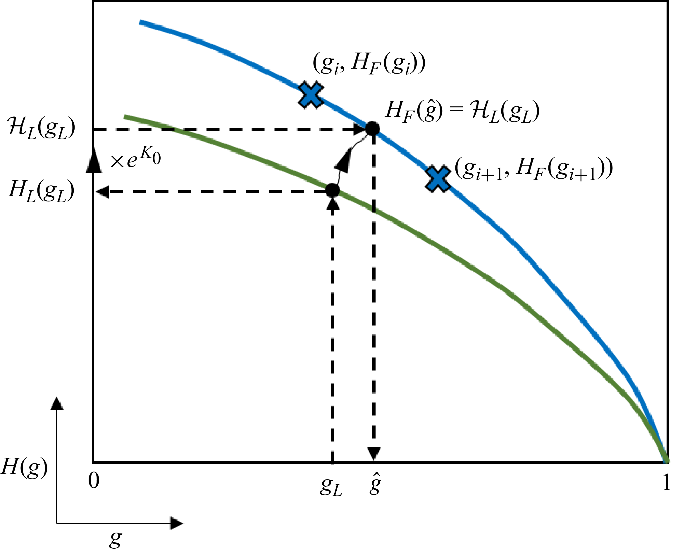
 g^
 HL
 gL
 HL
 HL=eK0HL
 g^
 HF

 ℓ0
 χ
 Rρ
 Cp
 g^(η^)
 gL(ηL)
 gF(ηF)
 TwL=100K
 TwF=1000K
 TeL=2935K
 TeF=3103K
 TwL=100K
 TwF=200K
 TeL=2935K
 TeF=4165K
 TwL=100K
 TwF=1000K
 TeL=2935K
 TeF=8586K

 dgF/dη|η=0
 dg^/dη|η=0
 Erel,∞Ω=||(g^−gF)/gF||L∞(Ω)×100
 Ω≡{0≤η≤1}

 C^p
 χ

 Open access

