2.0 MATHEMATICAL MODEL

2.1 Equations of motion

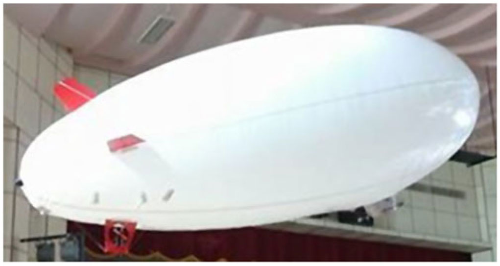
A high-altitude airship of pressure altitude 21km is considered in this work. This helium filled aerial vehicle is controlled using forward thrusters and control surfaces at the rear positioned in the cruciform tail configuration. Though stratospheric airship is considered in this work, a picture of low-altitude airship used in our laboratory for experimental purpose is shown in Fig. 1, for the ease of comprehension.

Figure 1.

Experimental airship.

The detailed study on the mathematical modelling of the considered airship was carried out in Refs. (Reference Gobiha and Sinha14,Reference Tiwari, Vora and Sinha15) and is presented in this section for the sake of completeness.

(1) \begin{align} \dot{V}&=\frac{1}{m_{x}}\left(T_{m}\eta\cos\alpha\cos\beta-\frac{1}{2}\rho V^2 SC_{D}-(mg-B)\sin\gamma\right)\nonumber\\[1pt] \dot{\alpha}&=q-\frac{1}{\cos\beta}\left(\left(\,p\cos\alpha+r\sin\alpha\right)\sin\beta\right.\nonumber\\[1pt] &\quad\ \ \,\left.+\,\frac{1}{m_{z}V}\left(\frac{1}{2}\rho V^2 SC_{L}+T_{m}\eta\sin\alpha - (mg-B)\cos\mu\cos\gamma\right)\right)\nonumber\\[1pt] \dot{\beta}&=\left(\,p\sin\alpha-r\cos\alpha\right)+\frac{1}{m_{y}V}\left(\frac{1}{2}\rho V^2 SC_{Y}-T_{m}\eta\sin\beta\cos\alpha +(mg-B)\sin\mu\cos\gamma\right)\nonumber\\[1pt] \dot{p}&=\left(\frac{J_{y}-J_{z}}{J_{x}}\right)qr+\frac{J_{xz}}{J_{x}}pq+\frac{1}{J_{x}}\left(\frac{1}{2}\rho V^2 SbC_{l}-Bb_{z}\sin\mu\cos\gamma\right)\nonumber\\[1pt] \dot{q}&=\left(\frac{J_{z}-J_{x}}{J_{y}}\right)pr+\frac{J_{xz}}{J_{y}}(r^2-p^2)+\frac{1}{J_{y}}\left(T_{m}\eta dz\cos\alpha\cos\beta+\frac{1}{2}\rho V^2 ScC_{m}-Bb_{z}\sin\theta\right)\nonumber\\[1pt] \dot{r}&=\left(\frac{J_{x}-J_{y}}{J_{z}}\right)pq-\frac{J_{xz}}{J_{z}}qr+\frac{\rho V^2 SbC_{n}}{2J_{z}}\nonumber\\[1pt] \dot{\phi}&=p+q\sin\phi\tan\theta+r\cos\phi\tan\theta\nonumber\\ \dot{\theta}&=q\cos\phi-r\sin\phi \end{align}

where

(2) \begin{align} \sin\gamma&=\cos\alpha\cos\beta\sin\theta-\sin\alpha\cos\beta\cos\phi\cos\theta -\sin\beta\sin\phi\cos\theta \nonumber\\ \sin\mu\cos\gamma&=\cos\alpha\sin\beta\sin\theta-\sin\alpha\sin\beta\cos\phi\cos\theta+\cos\beta\sin\phi\cos\theta\\ \cos\mu\cos\gamma&=\sin\theta\sin\alpha+\cos\alpha\cos\phi\cos\theta\nonumber\end{align}

2.2 Aerodynamic model

A aerodynamic model of the airship as used in Ref. (Reference Rana, Kumar, Sinha, Pal and Sati16) has been regarded and is tabulated below. As the entire regime of operation of aircraft is considered, all stability and control derivatives are taken as function of $\alpha$ .

(3) \begin{align} C_{L}&=C_{L_{0}}(\alpha)+C_{L_{q}}(\alpha)\frac{qc}{2V}+C_{L_{\delta_{e}}}(\alpha)\delta_{e}\nonumber\\[1pt] C_{Y}&=C_{Y_{\beta}}(\alpha)\beta+C_{Y_{p}}(\alpha)\frac{pb}{2V}+C_{Y_{r}}(\alpha)\frac{rb}{2V}+C_{Y_{\delta_{a}}}(\alpha)\delta_{a}+C_{Y_{\delta_{r}}}(\alpha)\delta_{r}\nonumber\\[1pt] C_{l}&=C_{l_{\beta}}(\alpha)\beta+C_{l_{p}}(\alpha)\frac{pb}{2V}+C_{l_{r}}(\alpha)\frac{rb}{2V}+C_{l_{\delta_{a}}}(\alpha)\delta_{a}+C_{l_{\delta_{r}}}(\alpha)\delta_{r}\nonumber\\[1pt] C_{n}&=C_{n_{\beta}}(\alpha)\beta+C_{n_{p}}(\alpha)\frac{pb}{2V}+C_{n_{r}}(\alpha)\frac{rb}{2V}+C_{n_{\delta_{a}}}(\alpha)\delta_{a}+C_{n_{\delta_{r}}}(\alpha)\delta_{r}\nonumber\\[1pt] C_{m}&=C_{m_{0}}(\alpha)+C_{m_{q}}(\alpha)\frac{qc}{2V}+C_{m_{\delta_{e}}}(\alpha)\delta_{e}\nonumber\\[1pt] C_{D}&=C_{D_{0}}(\alpha)+C_{D_{q}}(\alpha)\frac{qc}{2V}+C_{D_{\delta_{e}}}(\alpha)\delta_{e} \end{align}

Concisely, this work aims in estimating these derivatives from simulated flight data to establish an aero model for the considered airship.

(4) \begin{align} \Theta &=\left[C_{L_{0}} \ C_{L_{q}} \ C_{L_{\delta_{e}}} \ C_{Y_{\beta}} \ C_{Y_{p}} \ C_{Y_{r}} \ C_{Y_{\delta_{a}}} \ C_{Y_{\delta_{r}}} \ C_{l_{\beta}} \ C_{l_{p}} \ C_{l_{r}} \ C_{l_{\delta_{a}}} \ C_{l_{\delta_{r}}} \ C_{n_{\beta}} \ C_{n_{p}} \ C_{n_{r}} \ C_{n_{\delta_{a}}} \ C_{n_{\delta_{r}}} \ C_{m_{0}}\nonumber\right.\\ &\quad \left.C_{m_{q}} \ C_{m_{\delta_{e}}} \ C_{D_{0}} \ C_{D_{q}} \ C_{D_{\delta_{e}}}\right]^{T} \end{align}

3.0 GENERATION OF SIMULATED FLIGHT DATA

A prerequisite for nonlinear estimation using neural network is the availability of an exhaustive dataset ranging through the entire operating regime of the system. A dataset which spans entire operation regime is essential for this work because algorithms can learn and interpolate only within the trained regime. The use of extrapolated values based on the available dataset may lead to erroneous estimates especially when the system is nonlinear. As the real-time data is unavailable for the considered stratospheric airship model, data generation becomes vital for the estimation of airship parameters. Dataset should provide a global picture of trim states of the system as a function of control variables. This is accomplished in this work by carrying out standard bifurcation analysis using MATCONT continuation subroutine in the MATLAB^® environment.

The airship equation could be written as a set of nonlinear ordinary differential equations (as shown in Equation 1) of form,

(5) \begin{align} \dot{\textbf{x}}=\textbf{f}(\textbf{x},\textbf{u}), \end{align}

where x is the vector of state variables, and u is the vector of control variables. For the considered airship model, $\textbf{x} = [V, \alpha, \beta, p, q, r, \phi, \theta]^{T}$ and $\textbf{u}=[\eta, \delta_{e}, \delta_{a}, \delta_{r}]^{T}$ . For a fixed set of control variables, u, the system of equations specified in Equation (5) could be integrated to study the time response of x for a chosen initial condition. But it is extremely cumbersome to repeat the procedure for infinite set of initial conditions and control variables, u. Thus, the continuation algorithm is used to solve the above set of equations represented in Equation (5) as a function of single continuation parameter s chosen from u, while the remaining control variables p are fixed at the initial values, thus the above equation could be equivalently written as:

(6) \begin{align} \dot{\textbf{x}}=\textbf{f}(\textbf{x}, s, \textbf{p}=fixed) \end{align}

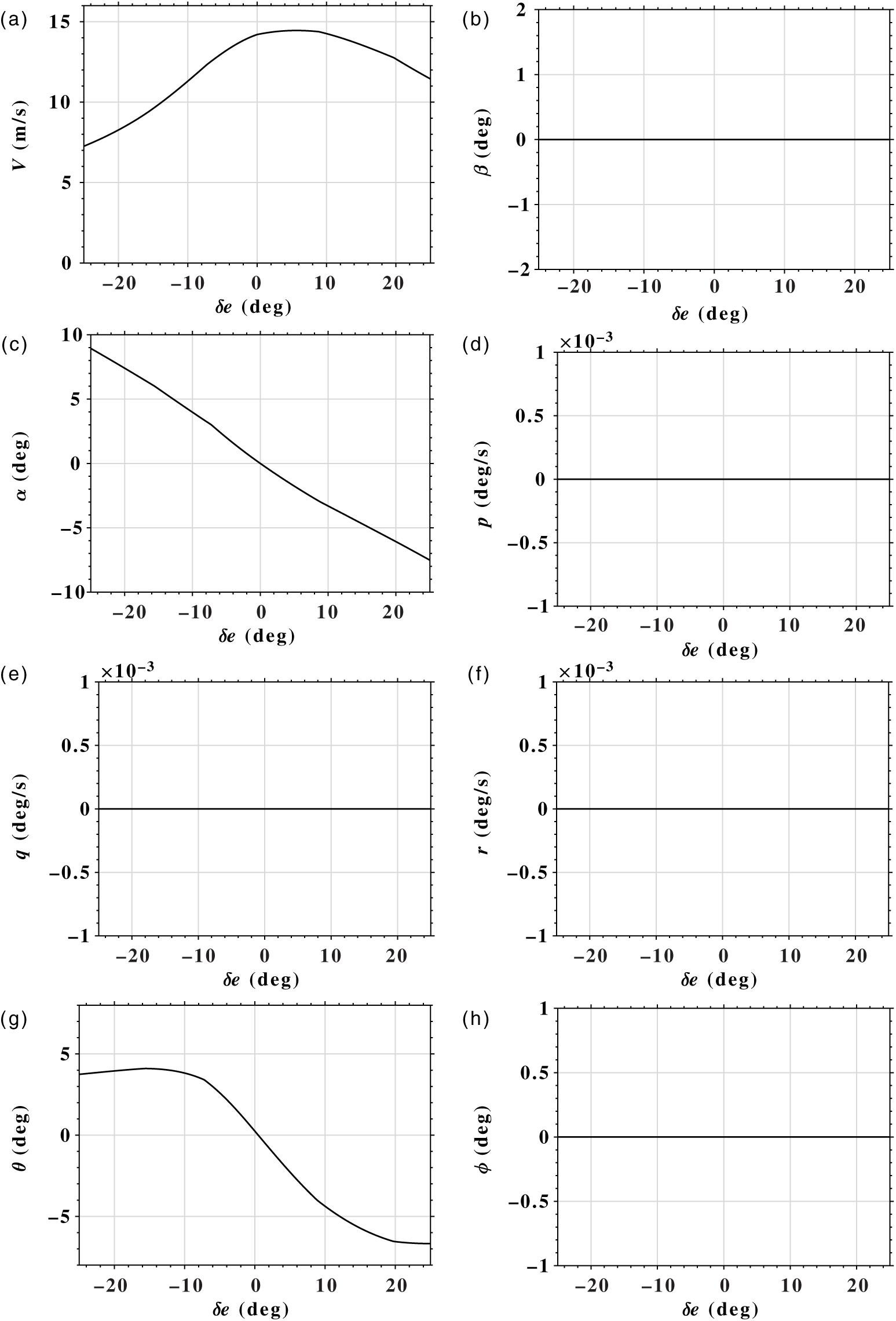
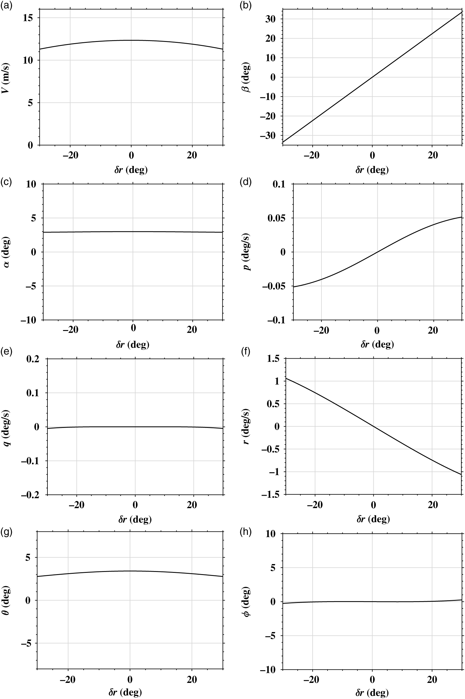
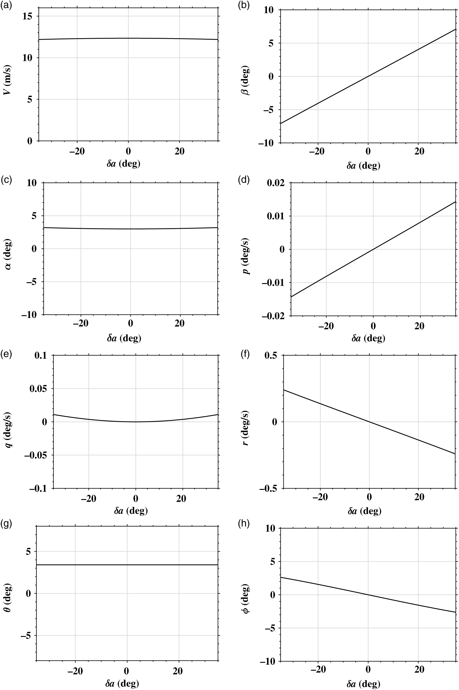
This depicts the response of states to change in control parameters, and such procedure is called standard bifurcation analysis. This generates all possible steady-state solutions called trim values throughout the flight regime with $\delta_{e}, \delta_{a}$ and $\delta_{r}$ as continuation parameters as shown in Figs 2, 3 and 4. Since engine thrust is almost maintained constant throughout the flight regime, $\eta$ continuation is not taken into consideration. The feasibility of the trim values are also accounted by constraining the continuation parameters with the bounds shown in Appendix A.3.

Figure 2.

Elevator continuation ( $\eta = 0.1836$ , $\delta_{{a}} = \delta_{{r}} = 0$ ).

Figure 3.

Rudder continuation ( $\eta = 0.1836$ , $\delta_{{e}} = -7.2135$ deg, $\delta_{\textit{a}} = 0$ ).

Figure 4.

Aileron continuation ( $\eta = 0.1836$ , $\delta_{\textit{e}} = -7.2135$ deg, $\delta_{\textit{r}} = 0$ ).

The obtained trim datasets are then used as initial conditions for generating flight data by open-loop simulation using fourth-order Runge–Kutta method. Simulation of the mathematical model in turn requires stability and control derivatives which are approximately computed using missile DATCOM software ^{(Reference Rana, Kumar, Sinha, Pal and Sati16)}. Missile DATCOM is a semi-empirical approach to predict the aerodynamics of the aerial vehicles based on its configuration. The modes of airship should be excited to generate time signals for reliable estimation. However, in this case, the response from the computed trim shows low magnitude oscillations as bifurcation analysis gives only the qualitative picture of the system. This makes it redundant to further excite the system for simulation.

Each row of datasets contains input and output sets for training the modular neural network. The input set consists of $\alpha$ , $\beta$ , $\frac{pb}{2V}$ , $\frac{qc}{2V}$ , $\frac{rb}{2V}$ , $\delta_{e}$ , $\delta_{a}$ and $\delta_{r}$ . The output set consists of aerodynamic coefficient values that are $C_{L}$ , $C_{D}$ , $C_{Y}$ , $C_{l}$ , $C_{m}$ and $C_{n}$ . The rows of datasets which are generated from different initial conditions are no longer time dependent. This is evident from the fact that parameters to be estimated do not change with time. Thus, datasets generated are combined to create training dataset.

The values of aerodynamic coefficients in each row of datasets could be obtained from DATCOM values for simulated flight data. But in this case, aerodynamic coefficient values are obtained by first calculating the rate of change of states using centrally pivoted five-point algorithm specified in Appendix A.2. Then, equations of motion (Equation 1) are solved for aerodynamic coefficients assuming that the true values of parameters are not known, as in case of real flight data. The DATCOM values are only used for generating simulated flight data.

4.0 PARAMETER ESTIMATION METHOD

4.1 Modular neural network

A modular network network is an ANN that constitutes independent neural networks connected by some intermediary. Each independent neural network or module carries out a sub-task of the global task attainable by the entire network. The intermediary integrates the output of each module to produce the required output. Modular neural networks are used when a complex task can be performed by breaking it into smaller viable tasks ^{(Reference Ding, Feng, Wang and Fu13)}. In this work, modular neural networks are trained separately to predict each aerodynamic coefficient, and the sub-task of estimating nonlinear parameters from angle of attack is achieved by independent modules using FFNN. FFNN is chosen as modules because they are considered universal function approximators, i.e. any nonlinear function can be computed and learnt by the network ^{(Reference Hornik, Stinchcombe and White7)}.

A multi-layer FFNN consists of neurons that are ordered into layers. The first layer is called the input layer, the last layer is called the output layer, and the layers in between are called hidden layers. Nodes in consecutive layers are connected with each other, and each connection is assigned a connective weight. The number of hidden layers and the number of nodes in each hidden layer is determined by the nonlinearity and complexity of the problem. Output of a layer is calculated by multiplying inputs with their respective weights. The resultants are then summed up, and the activation function is applied. Activation function provides nonlinear decision-making capability and is important for complex nonlinear functional mappings between input and output variables ^{(Reference Svozil, Kvasnicka and Pospichal17)}.

For parameter estimation of airship, the input variable to the module or FFNN is $\alpha$ and the response variable is unknown airship parameter from Equation (4). FFNN with one hidden layer was sufficient to capture nonlinearity in functions to be estimated. This is because one hidden layer with an arbitrarily large number of units suffices for the universal approximation property ^{(Reference Svozil, Kvasnicka and Pospichal17)}, and one hidden layer is used for aerospace applications in practice. Thus, each FFNN is composed of 1 node in input layer, 5 nodes in hidden layer and 1 node in output layer. Each node in one layer is connected to each node of the next layer (i.e. fully connected network). In this case, ‘softmax’ and ‘linear’ activation functions are used in the hidden layer and the output layer respectively of each module.

(7) \begin{equation} \begin{split} \text{Softmax activation,}\ \sigma(z)_{j}&=\frac{e^{z_{j}}}{\Sigma_{k=1}^{K} e^{z_{k}}}\ \text{for}\ j=1,..,K\\ \text{Linear activation,}\ f(x)&=ax \end{split} \end{equation}

where z is a vector (size=K) of the inputs to the output layer and j indexes the output units in softmax activation function. For linear activation function, x is an input and a is a constant.

These modules are then integrated with a dot product layer that is the final layer to predict an aerodynamic coefficient. Inputs for dot product layer are airship states, control inputs and outputs from modules. The number of modules and inputs are determined from Equation (3).

4.2 Training of network

For training, the network is initialised with weights that are small random numbers generated from uniform distribution. The output of the network is then compared with the available DATCOM values which were used for data generation. For comparison, mean squared error (MSE) is considered as the cost function. A cost function is a measure of performance of a neural network with respect to its given training sample and the expected output. The MSE for each iteration is defined by,

(8) \begin{align} MSE=\frac{1}{n}\Sigma_{i=1}^{n} (\hat{ Y_{i}}-Y_{i})^{2}, \end{align}

where $\hat{ Y}$ and Y are the desired and the predicted output of the modular neural network, respectively, and n is the batch size. Batch size is the number of samples that are to be propagated through the network.

The error calculated is propagated backward to the network using a method called back propagation. Back-propagation algorithm is used to compute gradient of a multi-variable function. In neural network, it computes gradient of the cost function which is a function of network weights and biases and uses gradient-descent algorithm to update the weights and bias terms iteratively such that the cost function is minimised. In this case, Adam optimisation algorithm ^{(Reference Kingma and Ba18)} is used instead of the classical stochastic gradient-descent procedure because it combines best properties of AdaGrad and RMSProp algorithms and can handle sparse gradients on noisy algorithms.

The training algorithm is iterative in nature. In each iteration, error is calculated, and the weights are updated using the number of samples in batch size. When all the training samples are passed through the algorithm, an epoch is completed. An epoch is a measure of number of times the entire available training samples are used to update the weights. The training sessions are continued until the MSE in successive iterations is decreasing. The predicted value is acceptable only if MSE is less than the minimum specified value. To achieve the desired level of MSE, hyperparameters of the network are tuned. Hyperparameters are variables that are set before optimising the model parameters. It determines the structure and training properties of the network. Hyperparameters of neural network algorithm are learning rate, loss function, batch size, epoch, number of hidden layer(s), number of units in the hidden layer(s) and type of activation functions which are adjusted by trial and error.

4.3 Estimation of longitudinal parameters

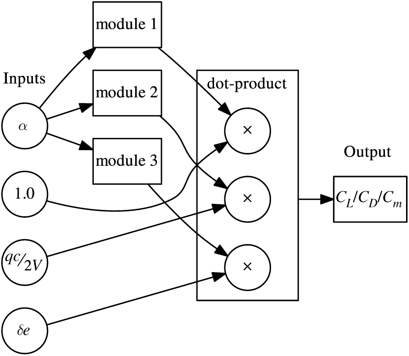
The architecture of modular neural network for estimation of longitudinal parameters of the airship is shown in Fig. 5. Network was trained on generated data for $C_{L}$ , $C_{D}$ and $C_{m}$ individually. Each module in the architecture is composed of 1 hidden layer with 5 nodes, as mentioned in the Subsection 4.1. Modules 1, 2 and 3 output $C_{x_{0}}$ , $C_{x_{q}}$ and $C_{x_{\delta_{e}}}$ parameters, respectively. The final layer computes dot product of the module outputs and airship states according to the following equation:

(9) \begin{equation} C_{x}=C_{x_{0}}+C_{x_{q}}\frac{qc}{2V}+C_{x_{\delta_{e}}}\delta_{e} \end{equation}

Figure 5.

Network architecture for longitudinal coefficients.

Once the modular neural network is trained satisfactorily to represent mapping of the input variables ( $\alpha$ , $\frac{qc}{2V}$ , $\delta_{e}$ ) to the output variable ( $C_{L}$ or $C_{D}$ or $C_{m}$ ), the network weights are fixed. Then, longitudinal parameters are estimated by passing on $\alpha$ values at each degree in the range $[{-15}^{\circ},{18}^{\circ}]$ . For these $\alpha$ inputs, the output of modules 1, 2 and 3 are recorded and plotted to compare with DATCOM values.

4.4 Estimation of lateral parameters

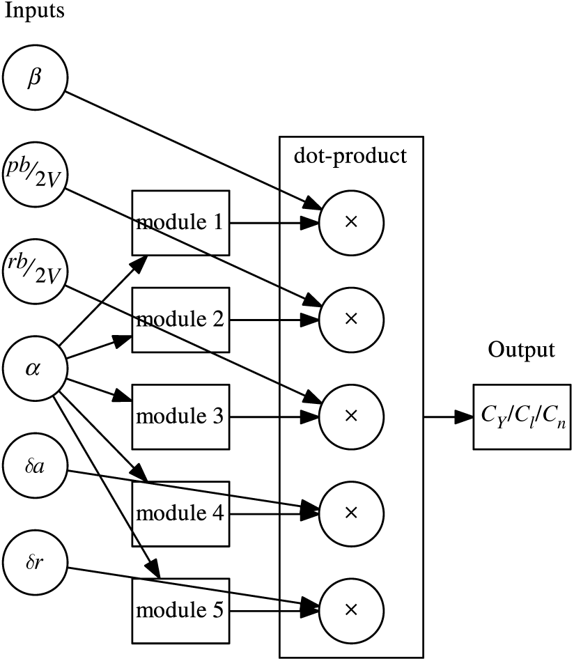
The network architecture for estimating lateral parameters is shown in Fig. 6. Modular neural network is trained for the aerodynamic coefficients, $C_{Y}$ , $C_{l}$ and $C_{n}$ , separately. Modules 1, 2, 3, 4 and 5 output $C_{x_{\beta}}$ , $C_{x_{p}}$ , $C_{x_{r}}$ , $C_{x_{\delta_{a}}}$ and $C_{x_{\delta_{r}}}$ parameters, respectively. The dot product is computed in the final layer according to the following equation:

(10) \begin{equation} C_{x}=C_{x_{\beta}}\beta+C_{x_{p}}\frac{pb}{2V}+C_{x_{r}}\frac{rb}{2V}+C_{x_{\delta_{a}}}\delta_{a}+C_{x_{\delta_{r}}}\delta_{r} \end{equation}

Figure 6:

Network architecture for lateral coefficients.

After networks are trained, parameters are estimated by passing $\alpha$ values at each one degree, similar to the longitudinal case.

5.0 RESULTS AND DISCUSSIONS

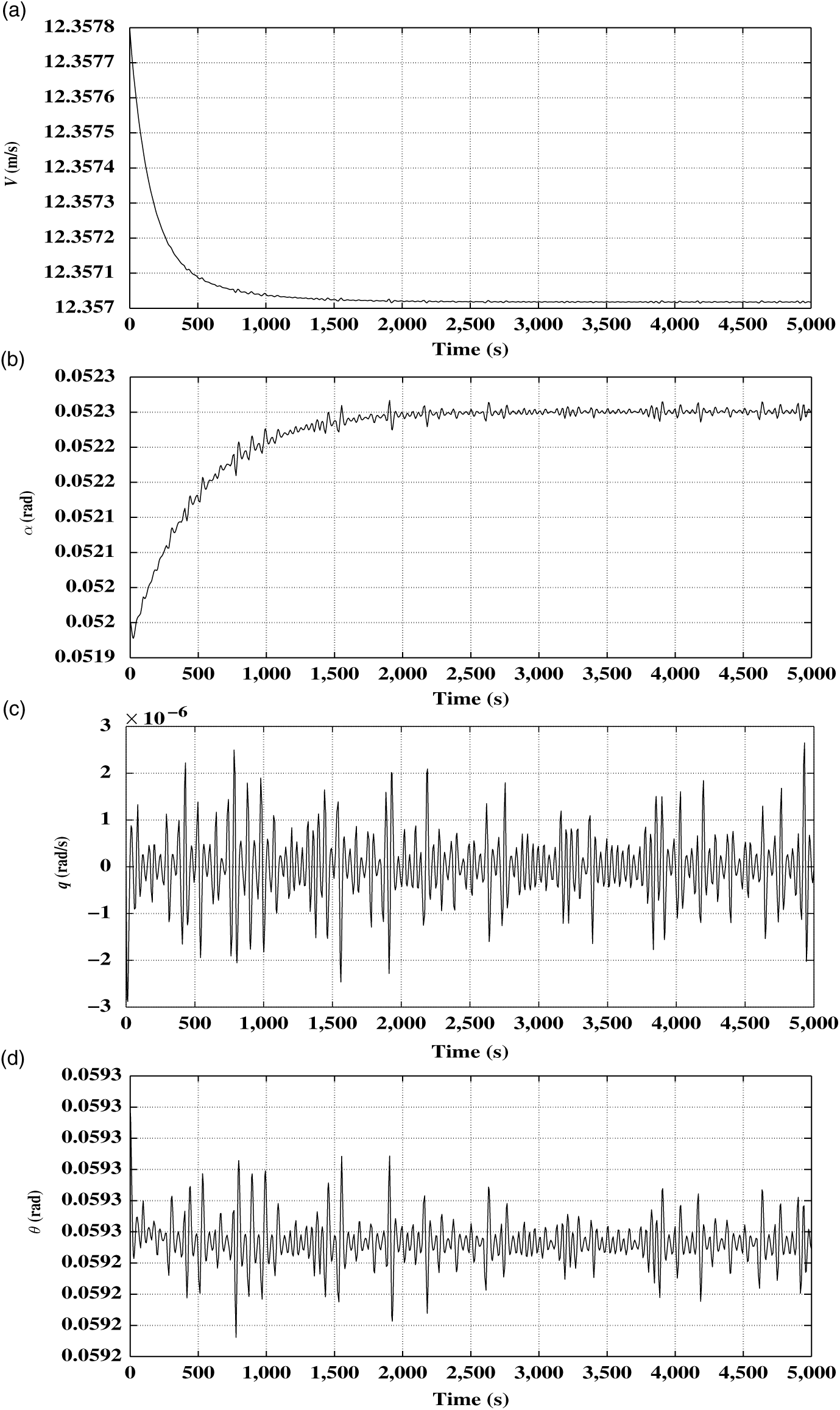
Data generation is a crucial phase of parameter estimation, as it has direct implication on performance. In this work, bifurcation-based continuation approach is relied on to compute all possible trim points. These trims are then taken as initial conditions, and airship is simulated for 5,000 seconds with the step size of 1 second. Figure 7 shows one such time simulation with initial condition taken from elevator continuation. The state vector, $\textbf{x}_{i}$ , and control vector, $\textbf{u}_{i}$ , corresponding to the considered initial condition are given by:

(11) \begin{align} \textbf{x}_{i}&=[12.3578, 0.0520, 0, 0, 0, 0, 0, 0.0593]^{T} \nonumber\\[3pt] \textbf{u}_{i}&=[0.1836, -0.1252, 0, 0]^{T} \end{align}

As evident from Fig. 7, there are low magnitude oscillations in longitudinal state variables. This excludes further excitation of the trim states, proving to be of major advantage as consideration on the type of excitation could be ignored. As $\delta_{a}$ and $\delta_{r}$ associated with the chosen trims are zero, lateral directional state variables are also zero and are not shown in Fig. 7. Thus, this analysis results in an extensive dataset of 4.5 million points which is used to effectively train the proposed neural network. As the trims are obtained from bifurcation plots, it spans the entire regime of operation of airship. This work is not regime specific and could be conveniently extended to real flight data, if available.

Figure 7:

Time simulation plots.

The generated dataset is split into two subsets: i.e. $75 \%$ for training and $25 \%$ for validation. Hyperparameters of neural network are tuned to obtain least training error for the training set, and the performance of trained network is validated on the validation set. In this work, training epoch and batch size are 1,000 and 5,000, respectively. Also, the training parameters for Adam optimization, i.e. learning rate, exponential decay rate for the first moment estimates ( $\beta_1$ ) and exponential decay rate for the second moment estimates ( $\beta_2$ ) are $10^{-4}$ , 0.9 and 0.999, respectively. Modular neural network for longitudinal and lateral coefficients has 48 and 80 trainable parameters, respectively. In every iteration, error is transmitted to modules because there is no trainable parameter in the dot product layer. Each module has 16 trainable parameters to be adjusted such that the MSE for the entire network is minimum. After training modular neural networks for each aerodynamic coefficient, MSE values are found to be in the order of $10^{-6}$ . Although MSE values are found to be of the same order for each modular neural network, it is higher for lateral aerodynamic coefficients in contrast to networks for longitudinal aerodynamic coefficients. This is because complexity or the number of trainable parameters are higher in modular neural networks for lateral aerodynamic coefficients.

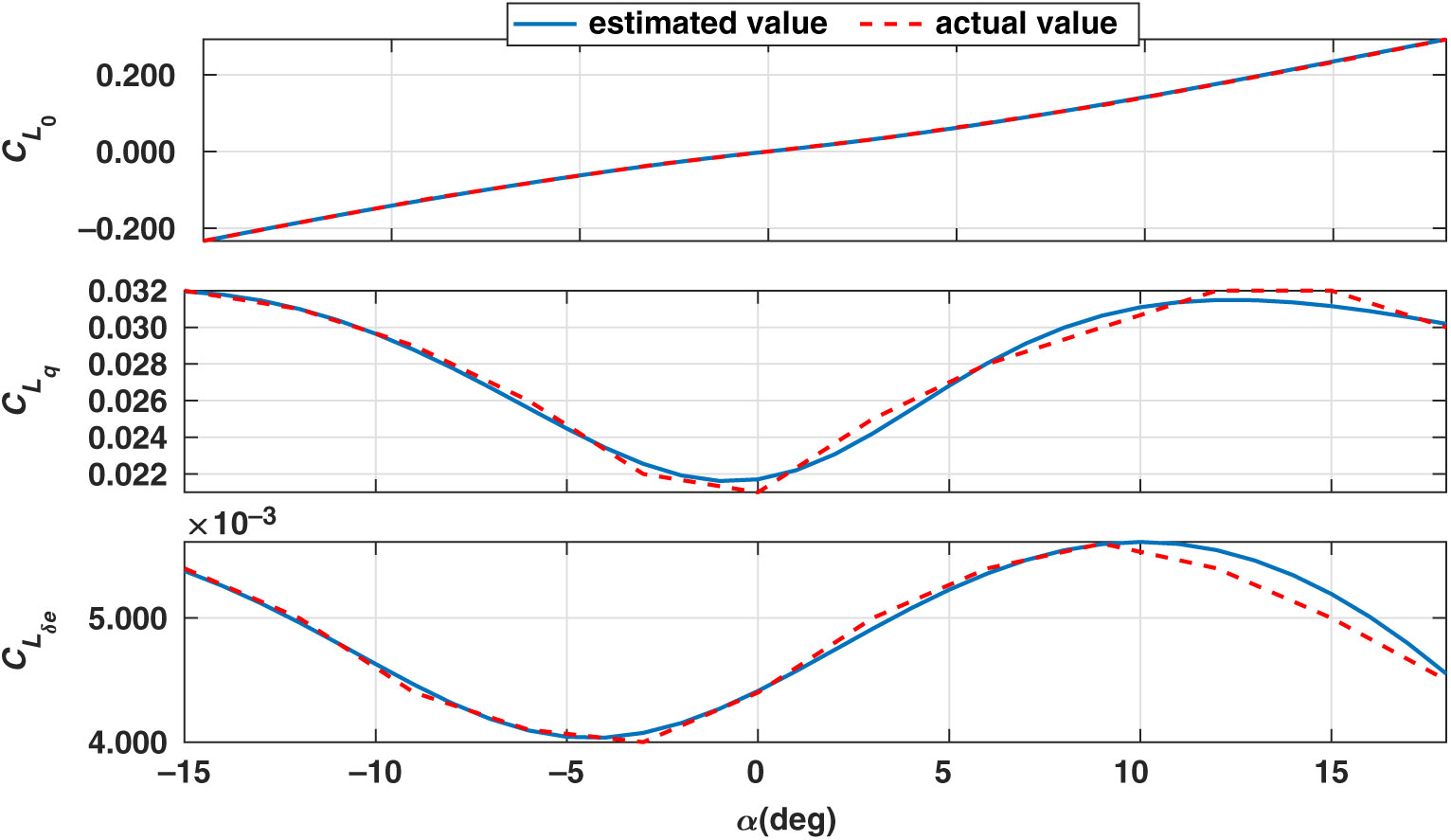
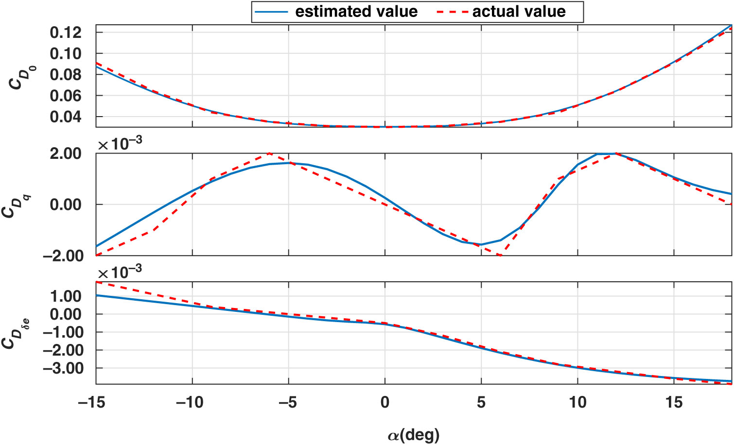
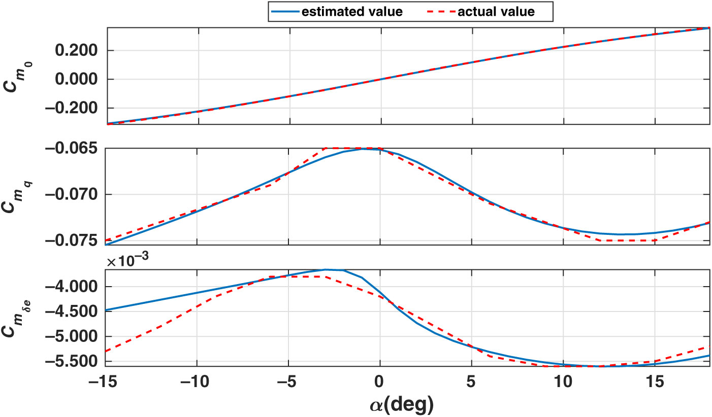
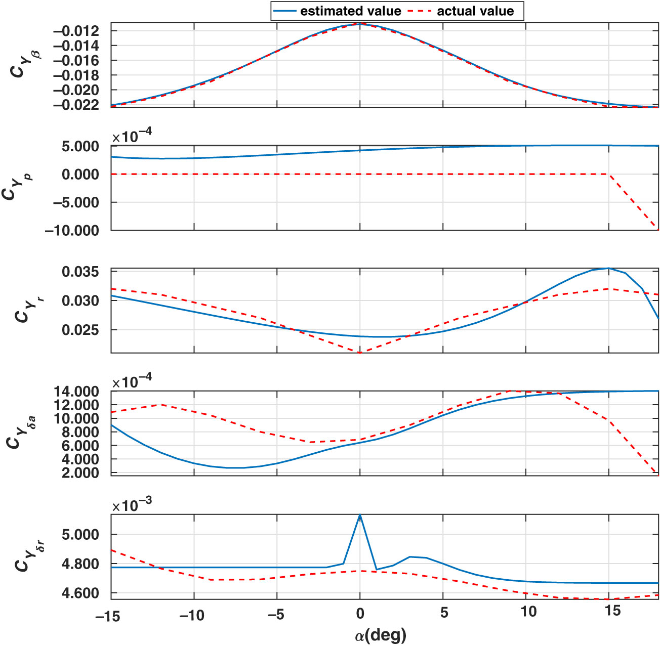
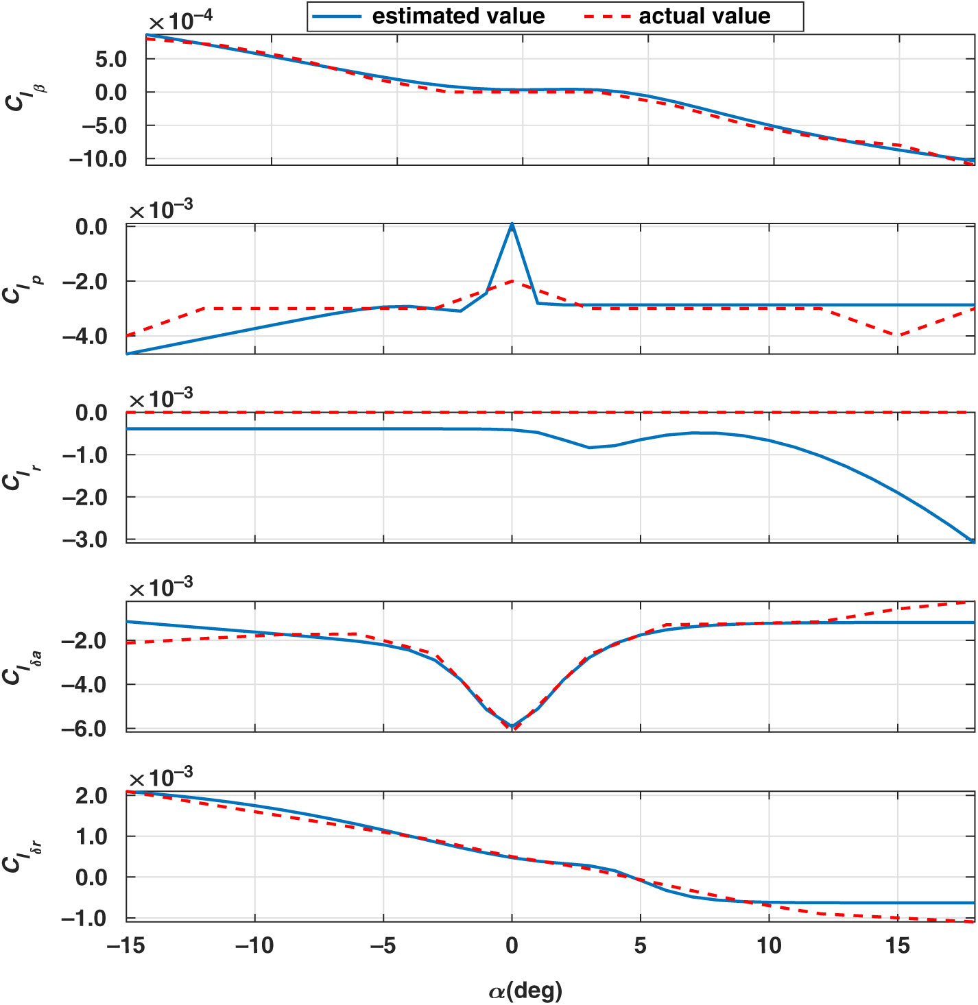
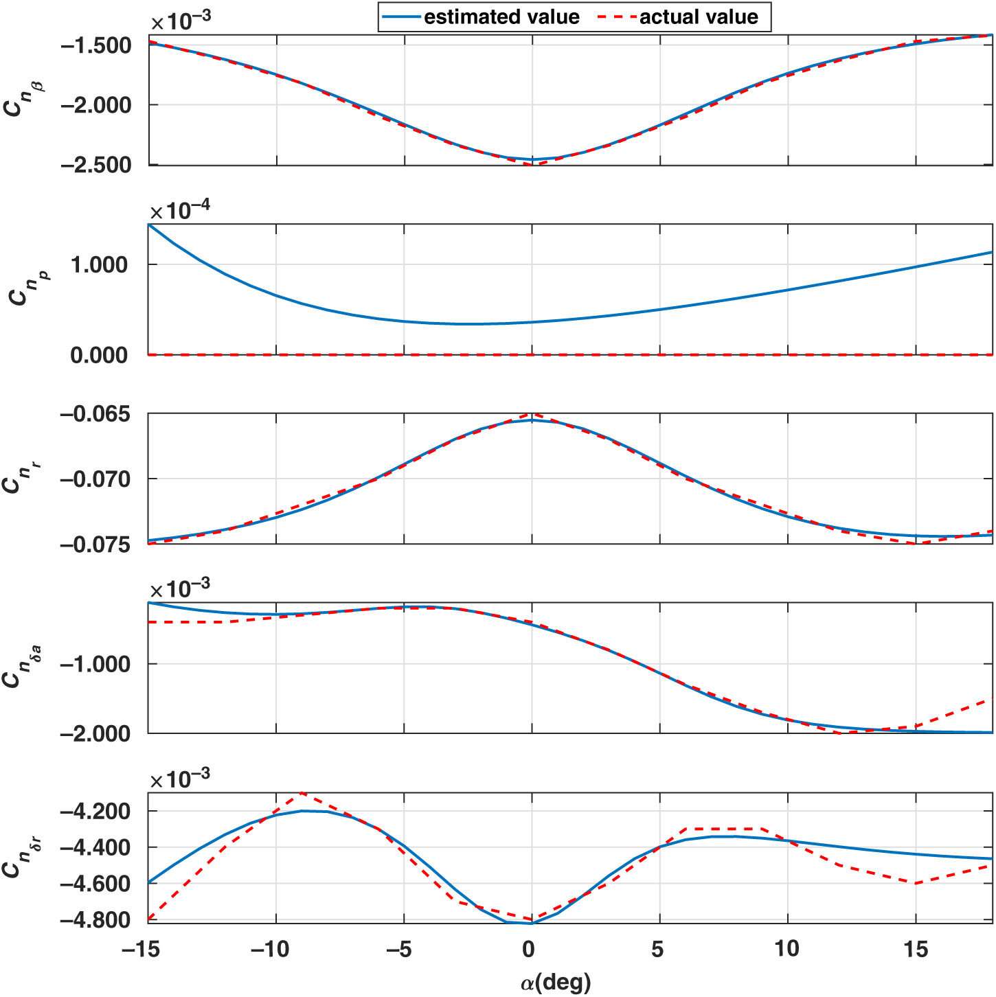
The neural network algorithm is implemented in Keras Python library which provides a clean and convenient way to create a range of deep learning models. The values of estimated and DATCOM parameters are plotted together to compare the performance of the proposed methodology. The DATCOM parameter values are considered as actual values in the plots because these values are used to generate simulated data which are then used for parameter estimation. In Figs 8, 9 and 10, the dashed lines (red) represent DATCOM or actual longitudinal parameter values and the solid lines (blue) represent estimated parameter values for $\alpha$ ranging from $[{-15}^{\circ},{18}^{\circ}]$ . Similarly, Figs 11, 12 and 13 present lateral parameters of the airship with solid lines (blue) depicting the estimated parameter values and dashed lines (red) representing DATCOM or actual parameter values.

Figure 8.

Derivatives of lift coefficient.

Figure 9.

Derivatives of drag coefficient.

Figure 10.

Derivatives of pitching moment coefficient.

Figure 11.

Derivatives of side force coefficient.

Figure 12.

Derivatives of rolling moment coefficient.

Figure 13.

Derivatives of yawing moment coefficient.

Since the aerodynamic model (Equation 3) is linear, classical estimation methods (mentioned in Section 1) such as least square could be used for estimation. But, it requires building different linear models for discrete values of $\alpha$ , and interpolation among these estimated values. However, the proposed nonlinear approach generates continuous plots of parameter values. It is worth mentioning that the fully connected FFNN trained on the same data has MSE values in the order of $10^{-4}$ . Modular neural network reduces the MSE significantly to $10^{-6}$ because it incorporates the mathematical form of the aerodynamic model in the network, whereas FFNN does not explicitly use aero modelling and rely entirely on a network to learn from data. Thus, the performance of modular neural network was found to be better than other neural network architectures and estimation algorithms.

As observed from the plots of stability and control derivatives, the estimated parameter values at both the ends slightly deviates from the actual value. This is predominantly attributed to insufficient data points in that regime. This evidently ascertains that the performance is greatly influenced by the available dataset or real flight data, if available. This is a limitation of the methodology, as real flight data might not be available for critical flight conditions because of safety aspects. However, this limitation is not applicable to unmanned aerial vehicles like an airship.

The estimated values as inferred from the plots are consistent with the assumed parameter values (i.e. missile DATCOM parameter values) used to generate simulated data. This validates the proposed methodology for estimating parameters of airship using simulated data and could be extended to real flight data of the airship without any change in neural network architecture. But, this might require addition of filters in the estimation procedure depending on the nature of measurement noise.