1 Introduction
The presence of vortex pairs over slender delta wings at high angle of attack has important effects on aerodynamic characteristics of manoeuvrable aircraft, and take-off and landing performance of supersonic aeroplanes (Lee & Ho Reference Lee and Ho1990). From the perspective of fundamental research, slender delta wings have relatively simple geometric shapes and few parameters, and the formation and evolution of the vortex pairs over them provide many interesting flow phenomena, including vortex breakdown, which are worth studying. Therefore, much attention has been paid to the studies of vortical flows around slender delta wings using theoretical, experimental and numerical methods.
Curved shear layers separated at the leading-edge roll up into concentrated vortices. Strong swirl velocity and jet-like axial velocity have been measured in the time-averaged vortex in the experiments, and are consistent with the theoretical models (Hall Reference Hall1961). The vortex flow has been assumed to be axisymmetric and conical by Hall (Reference Hall1961), which implies that the velocity components are functions of the conical parameter
 $r/x$
only (
 $r$
is the radial distance from the vortex axis and
 $x$
is the streamwise distance). There are also models that are based on the slender-body theory and the assumption of conical flow (Brown & Michael Reference Brown and Michael1954; Smith Reference Smith1968), in which the cross-flow velocity is a function of
 $s/x$
only (
 $s$
is the local semi-span). Various measurements show that the assumption of the conical flow is reasonable over slender delta wings as discussed by Hall (Reference Hall1961) and Smith (Reference Smith1968). Various unsteady flow phenomena of the vortices and the symmetry breaking of the vortex pair are reviewed below.
1.1 Shear layer instabilities
Flow separation from the leading edge and subsequent roll up of the three-dimensional curved shear layer into the leading-edge vortex are dominated by the Kelvin–Helmholtz instability (Gad-el-Hak & Blackwelder Reference Gad-el-Hak and Blackwelder1985; Gordnier & Visbal Reference Gordnier and Visbal1994; Cipolla & Rockwell Reference Cipolla and Rockwell1998). This instability is observed when the Reynolds number based on the chord length exceeds approximately
 $Re\approx 10^{4}$
. The three-dimensional nature of this instability has been studied by means of flow visualization, hot-wire velocity measurements, particle image velocimetry (PIV) measurements and direct numerical simulations. There is some disagreement in regard to the variation of the dominant frequency in the chordwise direction. Gordnier & Visbal (Reference Gordnier and Visbal1994) showed in their simulations that the shear layer frequency decreases in the chordwise direction, while the experiments of Gad-el-Hak & Blackwelder (Reference Gad-el-Hak and Blackwelder1985) do not confirm this, although their wings cannot be classified as slender delta wings.
As reviewed by Gursul (Reference Gursul2005), it is possible that disturbances in individual facilities may affect the frequency of the instability due to the shear layers being unstable in a band of frequencies. Nevertheless, simulations (Gordnier & Visbal Reference Gordnier and Visbal1994) suggest that the linear stability analysis of the shear layer in a cross-flow plane can predict the dominant frequencies.
1.2 Vortex instabilities
With increasing angle of attack vortex breakdown phenomenon is observed, where the axial flow becomes wake-like (Leibovich Reference Leibovich1984) and strong unsteadiness develops (Gursul Reference Gursul1994). The occurrence and mechanisms of vortex breakdown have been debated and different explanations have been offered as reviewed by Leibovich (Reference Leibovich1984) and Delery (Reference Delery1994). Linear temporal stability analysis of realistic delta wing flows confirmed that helical modes are destabilized downstream of the breakdown, but the perturbations are stabilized or weakly amplified upstream of the breakdown (Renac & Jacquin Reference Renac and Jacquin2007). The helical mode instability downstream of the breakdown was confirmed by two-point unsteady pressure measurements (Gursul Reference Gursul1994) and instantaneous azimuthal vorticity distribution in a plane that passes through the vortex axis (Towfighi & Rockwell Reference Towfighi and Rockwell1993). The dominant frequency of the helical mode instability of flow downstream of breakdown is smaller than that of the shear layer instability and also exhibits a decrease in the chordwise direction. In this paper, we will mostly focus on the flow upstream of breakdown or in the absence of breakdown on the wing.
Although time-averaged vortex flow upstream of breakdown appears to be stable, the flow can be highly unsteady. Large velocity fluctuations, due to the displacements of the vortex core, attributed to ‘meandering’ or ‘wandering’, were observed well upstream of vortex breakdown and also in the absence of breakdown on the wing (Menke & Gursul Reference Menke and Gursul1997). The meandering mode has been captured on a simple delta wing with a sweep angle of
 $\unicode[STIX]{x1D6EC}=70^{\circ }$
by means of the proper orthogonal decomposition (POD) analysis (Zhang, Wang & Gursul Reference Zhang, Wang and Gursul2016). The most energetic mode exhibited a vortex dipole centred on the time-averaged vortex. In the second most energetic mode, another vortex dipole was found, which was orthogonal to the one in the first mode. A linear combination of these eigenmodes represents displacements of the vortex core in the helical mode with an azimuthal wavenumber of
 $m=1$
. The same first helical mode was identified in the experiments on trailing vortices (Roy & Leweke Reference Roy and Leweke2008; Del Pino et al.
Reference Del Pino, Lopez-Alonso, Parras and Fernandez-Feria2011). Slender delta wing vortices studied in this paper (for
 $\unicode[STIX]{x1D6EC}\geqslant 75^{\circ }$
) have not been analysed by the POD method in previous research, however we expect the meandering mode to be affected as the sweep angle increases. This is based on the POD analysis of the afterbody vortices from a slanted axisymmetric cylinder (Bulathsinghala et al.
Reference Bulathsinghala, Jackson, Wang and Gursul2017). It was found that, as the upsweep angle increases, the helical mode representing the meandering has an increasing percentage of the total energy.
1.3 Symmetry breaking
A much debated and still open issue is the symmetry breaking of the vortex pair over slender delta wings. There have been conflicting experimental observations and interpretations on the existence and nature of the symmetry breaking over slender delta wings. Early observations (Birds Reference Birds1969) and analysis of the rolling-moment data (Polhamus Reference Polhamus1971) suggested that the vortex pair becomes asymmetric with increasing angle of attack
 $\unicode[STIX]{x1D6FC}$
and sweep angle
 $\unicode[STIX]{x1D6EC}$
. The boundary of vortex asymmetry, also called ‘vortex contact’ by Polhamus (Reference Polhamus1971), has been reproduced in the literature many times. The occurrence of symmetry breaking on delta wings has some similarity to well-known vortex asymmetry on bodies of revolution (Tobak & Peake Reference Tobak and Peake1982). Keener & Chapman (Reference Keener and Chapman1977) suggested that the vortex pair asymmetry on slender bodies of revolution and slender delta wings is created by the same ‘hydrodynamic instability’ resulting from the ‘crowding’ together of the vortices.
However, these observations and interpretations have been challenged by the theoretical models and other experiments. Based on the slender-body theory, Lowson & Ponton (Reference Lowson and Ponton1992) predicted that there is increasing resistance to asymmetry for thinner cross-sections, and that flow on an ideal delta wing with zero thickness would remain symmetric. They also carried out experiments for delta wings with sweep angles
 $\unicode[STIX]{x1D6EC}=70^{\circ }$
and
 $80^{\circ }$
, and did not observe any vortex asymmetry. Therefore they suggested that previously reported asymmetries might be due to the thickness of the apex of the models. Stahl, Mahmood & Asghar (Reference Stahl, Mahmood and Asghar1992) also did not observe any asymmetries before vortex breakdown occurred on wings with sweep angles
 $\unicode[STIX]{x1D6EC}=82^{\circ }$
and
 $86^{\circ }$
. Additional support in favour of symmetric flows over slender delta wings came from stability analysis of the point-vortex pair, using conical-flow assumptions and slender-body theory (Huang & Chow Reference Huang and Chow1996; Cai, Liu & Luo Reference Cai, Liu and Luo2003). Introducing small amplitude disturbances decomposed into four basic modes (displacements of the vortices being in either the same or opposite directions), it was found that the vortex pair is always stable for the parameter range studied. In these studies, the main wing parameter is the Sychev similarity parameter:
 $$\begin{eqnarray}K=\frac{\tan \unicode[STIX]{x1D6FC}}{\tan (90^{\circ }-\unicode[STIX]{x1D6EC})}.\end{eqnarray}$$
This parameter appears in the modelling of conical-flow fields with point vortices and vortex sheets by means of complex variables (Smith Reference Smith1968; Huang & Chow Reference Huang and Chow1996; Cai et al.
Reference Cai, Liu and Luo2003). The magnitude of the cross-flow component of the axial velocity is inversely proportional to the parameter
 $K$
. This velocity component can be considered to pull the vortex toward the symmetry plane and stabilize the vortex pair (Huang & Chow Reference Huang and Chow1996). As the magnitude of this component decreases with the similarity parameter
 $K$
, one would expect stability to diminish with increasing
 $K$
, which occurs either by increasing the angle of attack or by increasing the sweep angle. The point-vortex pair was found to be stable for
 $K\leqslant 2.0$
by Huang & Chow (Reference Huang and Chow1996), and later on for
 $K\leqslant 10.0$
by Cai et al. (Reference Cai, Liu and Luo2003), although the degree of stability decreases with increasing
 $K$
. In contrast, with increasing thickness of elliptic cones, the symmetric vortex pair becomes unstable (Cai et al.
Reference Cai, Liu and Luo2003). Hence, the temporal stability analysis of the point-vortex pair appears to support the suggestions that the thickness near the apex of the model might cause the flow asymmetry in the experiments.
However, recent experiments (Wu, Deng & Wang Reference Wu, Deng and Wang2014) on a sharp-edged thin delta wing with
 $\unicode[STIX]{x1D6EC}=85^{\circ }$
suggested that an asymmetric vortex may be present before vortex breakdown appears on the wing. In another study (Lim, Lua & Luo Reference Lim, Lua and Luo2001) it was found that not only was vortex asymmetry observed on thin plate wings, but also that there was no relation to the breakdown. Even when one of the vortices exhibits vortex breakdown on the wing, the vortex pair may be symmetrical up to the point of vortex breakdown or develop significant asymmetry well upstream of breakdown. In the light of these recent experiments, the apparent inconsistency between the temporal stability analysis of the point-vortex pairs and observations may originate from the oversimplification of the structure of real vortices. In addition, it is not certain to which degree the location and strength of the point vortices agree with the experiments. After all, this may not be a suitable approach to explain symmetry breaking on thin delta wings with sharp edges. It is noted that, in the case of bodies of revolution, there is experimental and computational evidence that a convective instability of the originally symmetric flow can explain the vortex asymmetry (Degani Reference Degani1991; Degani & Tobak Reference Degani and Tobak1992). A small disturbance due to geometric imperfections near the nose grows in the streamwise direction. It is not clear why the initial small perturbation grows by several orders of magnitude and also whether this instability exists for thin wings with fixed separation points.
1.4 Instabilities of vortex pairs
It is unclear whether the instabilities of vortex pairs play any role in the onset of symmetry breaking. The works of Huang & Chow (Reference Huang and Chow1996) and Cai et al. (Reference Cai, Liu and Luo2003), using point vortices in the conical flow and slender-body theory, represent the infinitely long wavelength limit in the stability analysis. The ratio of the vortex radius
 $a$
to the vortex separation
 $b$
is an important parameter with regard to the instabilities of vortex pairs. According to studies of parallel vortex pairs (as opposed to conical pairs for which both the vortex radius
 $a$
and vortex separation distance
 $b$
increase linearly in the streamwise direction), both long wavelength and short wavelength instabilities can be amplified (Leweke, Le Dizés and Williamson Reference Leweke, Le Dizés and Williamson2016). For the long wavelength (Crow) instability, the most unstable wavelengths are between
 $\unicode[STIX]{x1D706}/b$
 ${\approx}$
6 and 8 for
 $0.1\leqslant a/b\leqslant 0.3$
. On the other hand, it is expected that the short wavelength (elliptic) instability scales on the core radius. For parallel vortex pairs in the range of
 $0.1\leqslant a/b\leqslant 0.3$
, the counter-rotating vortex pair becomes unstable above a critical Reynolds number
 $\unicode[STIX]{x1D6E4}/\unicode[STIX]{x1D708}$
, which is of the order of
 $10^{2}$
to
 $10^{3}$
(Leweke et al.
Reference Leweke, Le Dizés and Williamson2016).
To the best of our knowledge, there have been no studies on the interactions between the vortices of the vortex pairs on delta wings, correlation between the unsteady flow in the vortices and possible relation to vortex-pair instabilities and symmetry breaking. It is interesting that vortex breakdown location over delta wings is not steady and exhibits low-frequency quasi-periodic fluctuations along the vortex axis as observed in several experiments (Gursul & Yang Reference Gursul and Yang1995). An interesting aspect is that the breakdown locations of the left and right vortices oscillate out-of-phase (Menke, Yang & Gursul Reference Menke, Yang and Gursul1999), revealing that there might be interactions between the vortices of the conical vortex pairs.
1.5 Objectives of this study
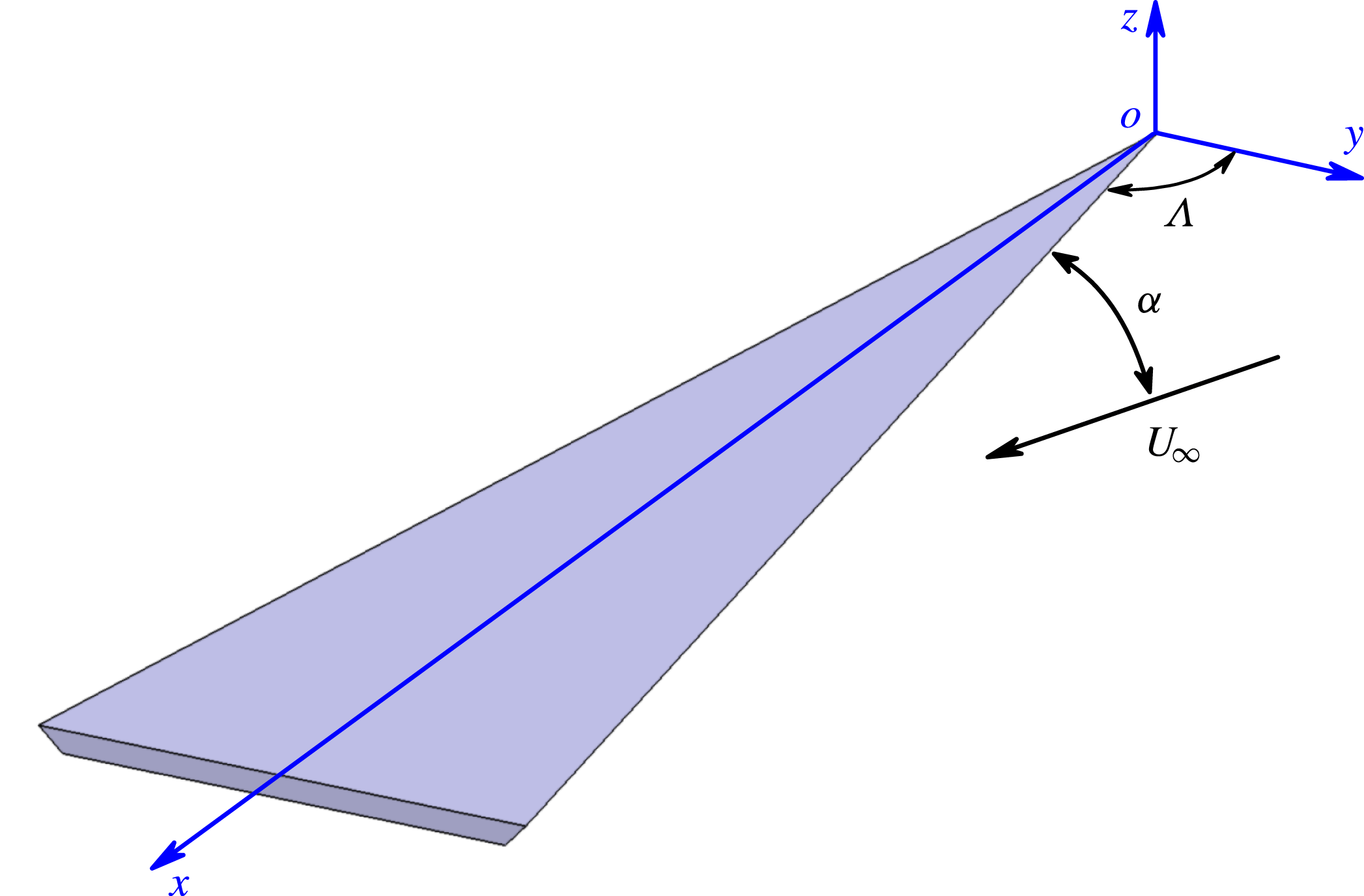
In view of inconsistencies of the previous experimental results and the unclear relation to theoretical explanations, we carried out an experimental investigation of conical vortex pairs over slender delta wings. Water tunnel experiments are conducted for three delta wings of
 $75^{\circ }$
,
 $80^{\circ }$
and
 $85^{\circ }$
sweep angle (see figure 1) using two dimensional particle image velocimetry measurements. We show that whether the time-averaged vortex pair exhibits asymmetry or not depends on a single parameter: the Sychev similarity parameter
 $K$
. We also investigated the most energetic modes of the unsteady flow field by means of proper orthogonal decomposition and the quasi-periodic oscillatory modes by means of dynamic mode decomposition (DMD) methods. These were used to investigate the shear layer instabilities and the vortex instabilities.
Schematic of slender delta wing.

2 Experimental techniques
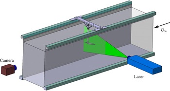
The experiments were conducted in a closed-loop water tunnel with a test section 381 mm wide and 508 mm deep and a maximum flow speed of
 $0.5~\text{m}~\text{s}^{-1}$
. The schematic of the experimental set-up is shown in figure 2. The tunnel has four viewing windows, three surrounding the test section and one downstream that allows viewing of the cross-flow planes. The delta wing models were installed upside down in the water tunnel. The support was connected to the lower surface of the wings, keeping the leeward flow unaffected. The stiffness of the support was carefully considered during the design to avoid model vibrations; no vibration was observed in the experiments. The models were painted matt black in order to reduce reflections from the laser sheet during the particle image velocimetry measurements. The maximum blockage of models in the water tunnel is approximately 1.7 % for the
 $75^{\circ }$
sweep wing at the maximum angle of attack of
 $40^{\circ }$
.
Schematic of experimental set-up.

Three models of slender delta wings with leading-edge sweep angles of
 $\unicode[STIX]{x1D6EC}=75^{\circ }$
,
 $80^{\circ }$
and
 $85^{\circ }$
were used in the experiments. The chord length of all three wings was fixed at
 $c=250~\text{mm}$
. The wing models were manufactured from aluminium sheet and had a thickness of 4 mm and
 $45^{\circ }$
leading-edge bevel. Based on the data in the literature, it was expected that vortex breakdown would not be observed on the wing until
 $\unicode[STIX]{x1D6FC}=35$
to
 $40^{\circ }$
for these slender delta wings. Therefore, the range of angles of attack in the experiments was selected to be from
 $15^{\circ }$
to
 $40^{\circ }$
with an interval of
 $5^{\circ }$
. The Reynolds number based on the root chord length of wings is
 $0.9\times 10^{5}$
. The coordinate system definition for slender wings is shown in figure 1.
Particle image velocimetry measurements were carried out with a TSI PIV system which has dual 120 mJ Nd:Yag lasers. The water flow was seeded with
 $4~\unicode[STIX]{x03BC}\text{m}$
hollow glass particles. The laser sheet illuminated the cross-flow fields from the side of the water tunnel and was perpendicular to the free stream direction, and the camera was located downstream to view the cross-flow planes through the viewing window. Measurements were taken at three cross-flow planes:
 $x/c=0.5$
, 0.75 and 1.0. Images were taken using a 4M digital camera (12 bit,
 $2048\times 2048$
pixels). Insight 3G image processing software and dual processor Xeon computer were used for PIV data processing. Image pairs were correlated to obtain particle displacement and, then, velocity fields. The
 $24\times 24$
pixels interrogation windows were used with a 25 % window overlap, and the associated grid size was approximately
 $0.3\,\%c$
. For each case, a sampling rate of 15 Hz was used in experiments, and 1000 instantaneous snapshots were taken for each case. Uncertainty in the velocity data was estimated to be approximately 2 %.
Unlike trailing vortices in the far wake, there is often vorticity of opposite sign around the leading-edge vortices as they develop over the wing. For the calculation of circulation, the area integral of the vorticity was used because this offers an easy way to exclude the secondary vorticity of opposite sign. If the line integral of velocity were used for the calculation of circulation, the determination of the integral path separating the opposite sign of vorticity would be difficult. In our calculations, the time-averaged vorticity was calculated from the time-averaged velocity field using second-order central differencing. The calculation of the circulation was continued by addition of the vorticity until a small threshold value of vorticity was reached. In our experience of using PIV data, the two methods, based on the line integral of velocity and area integral of vorticity, do not differ much. The vorticity has larger uncertainty, however the velocity magnitude used in the line integral is small when away from the core, leading to larger relative error. We estimate the uncertainty of the circulation to be approximately 6 %.
Two different methods were employed to calculate the vortex core size. The first one is based on the time-averaged flow fields, and the second one is based on the ensemble average of the instantaneous flow fields. Both methods employ the second-order moment of vorticity to calculate the core size based on the vorticity fields. In the first method, the calculation of the vorticity is based on the averaged velocity fields. The averaged velocity fields are smooth enough, therefore second-order central differencing is used as suggested by Raffel et al. (Reference Raffel, Willert, Wereley and Kompenhans2007). In the second method, vorticity in the calculation of the vortex core size was obtained by a different method. First, the local circulation around the point is calculated, and then the average vorticity is obtained from the local circulation and the area enclosed by the integral path. Since the instantaneous velocity fields consist of background noise, this ‘circulation method’ is more robust (Raffel et al. Reference Raffel, Willert, Wereley and Kompenhans2007).
During the post-processing, the time-averaged flow fields, POD modes and DMD modes were calculated to reveal the flow characteristics. The POD analysis is a well-known tool for analysing unsteady flows by expanding a random function as a series of deterministic functions with random coefficients so that it is possible to separate the deterministic part from the random one. This is used to capture the most energetic structures of the flow (Lumley Reference Lumley1970). The energy of stochastic signal is given by the sum of the eigenvalues so that each eigenvalue taken individually represents the energy contribution of the corresponding deterministic function. The modes are ranked according to their kinetic energy, and the first POD mode is then the one with the highest kinetic energy. A snapshot POD proposed by Sirovich (Reference Sirovich1987) was utilized in the present calculations, which decomposed the instantaneous velocity fields as a spatial vector function and extracted the most energetic eigenfunction. The POD analysis was implemented using the TSI Grad-POD Toolbox, which employs the spatio-temporal data analysis technique proposed by Heiland (Reference Heiland1992).
The DMD analysis, which was first proposed by Schmid (Reference Schmid2010) and rapidly developed in recent years, is also a useful method to find coherent structures in complex flow fields. The dynamic mode decomposition attempts to find distinct frequencies in the spatial data. As the DMD method decomposes the spatial flow fields by frequencies, it is very suitable to analyse periodic flows. For linear processes, DMD modes represent the global stability modes. For time-periodic flows, DMD modes reduce to Fourier modes. In the case of uniformly sampled PIV measurements, the dynamic mode decomposition can be used to identify not only the dominant frequencies, but also the spatial structure of these modes. The current DMD code is based on the algorithm proposed by Tu et al. (Reference Tu, Rowley, Luchtenburg, Brunton and Kutz2014) and has been verified and validated. The convergence testing indicated that 1000 snapshots are adequate for the DMD analysis in our case.
3 Results and discussion
3.1 Time-averaged vortex pairs
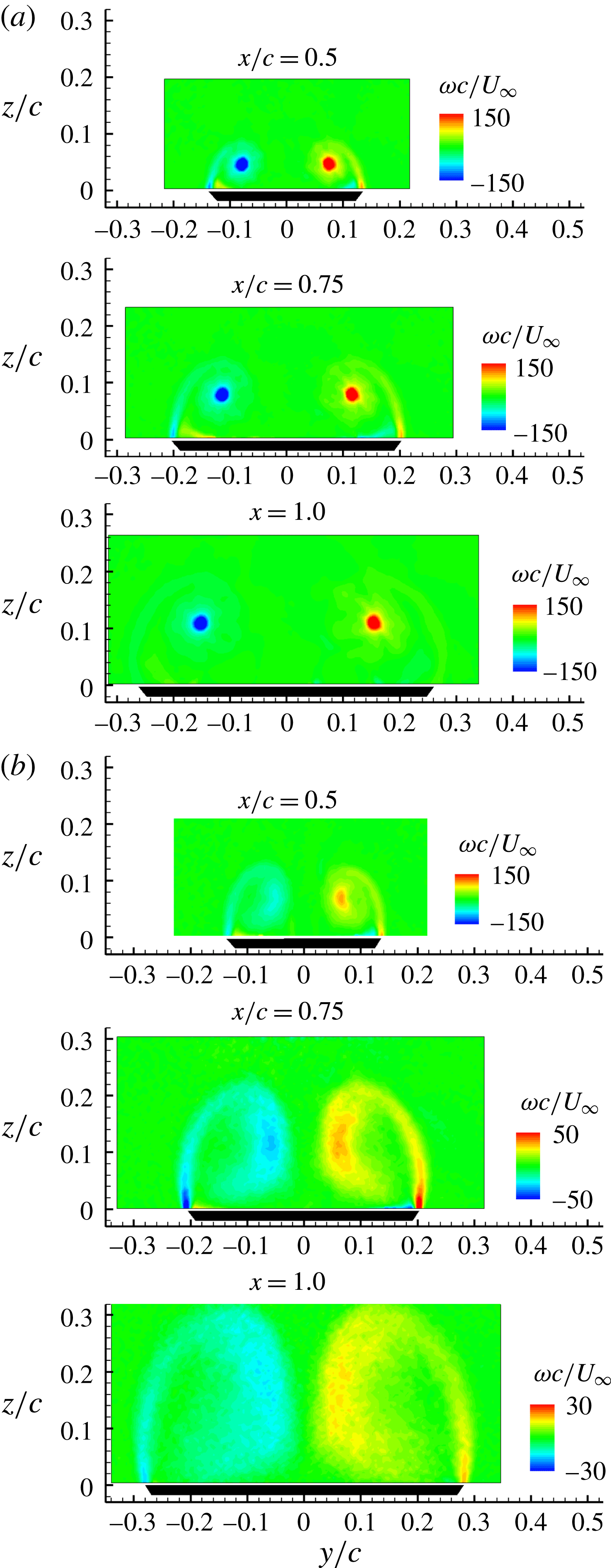
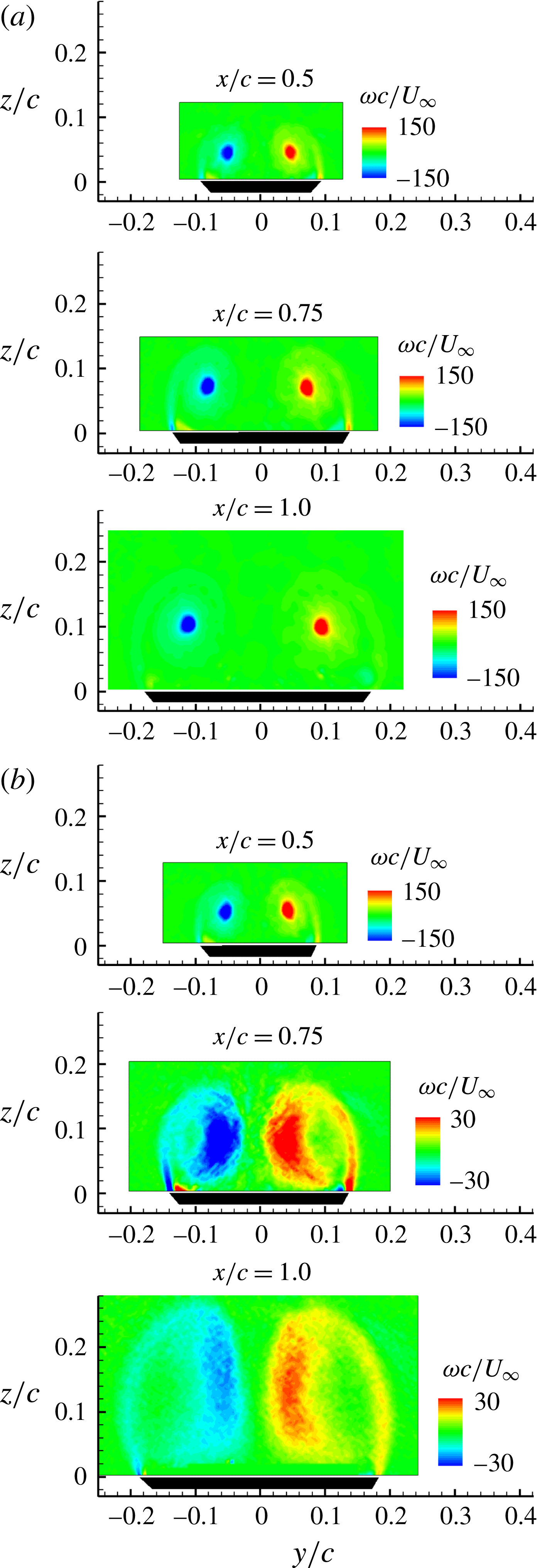
For slender delta wings with sharp edges, the vortex pairs are formed at relatively low angles of attack, and the vortices become stronger with increasing angle of attack. The time-averaged structures of the vortex pairs are relatively simple before breakdown. Figure 3 shows the time-averaged vorticity distributions for the
 $75^{\circ }$
sweep wing at
 $\unicode[STIX]{x1D6FC}=30^{\circ }$
and
 $40^{\circ }$
. The vorticity is normalized by the chord length
 $c$
and free stream speed
 $U_{\infty }$
. At
 $\unicode[STIX]{x1D6FC}=30^{\circ }$
, a symmetric vortex pair is observed at all three measurement planes and there is no breakdown. The distance between the vortices and the distance of the vortices from the wing surface appear to increase linearly with increasing chordwise distance. At
 $\unicode[STIX]{x1D6FC}=40^{\circ }$
, however, the vortex breakdown has moved upstream of the measurement plane at
 $x/c=0.5$
, and it is interesting that the time-averaged vortex structures after breakdown are still roughly symmetric (no significant asymmetry). The vorticity contours after breakdown are displayed with different scales for different planes for clarity of the vortex patterns, because the vortex cores expand after breakdown and the vorticity magnitude decreases substantially at downstream stations. The vorticity fields for the most downstream measurement plane
 $(x/c=1.0)$
of the
 $75^{\circ }$
sweep wing are illustrated in figure 4(a) for angles of attack of
 $30^{\circ }$
,
 $35^{\circ }$
and
 $40^{\circ }$
. For the smallest angle of attack, the vortex pair is symmetric and has no breakdown. For
 $\unicode[STIX]{x1D6FC}=35^{\circ }$
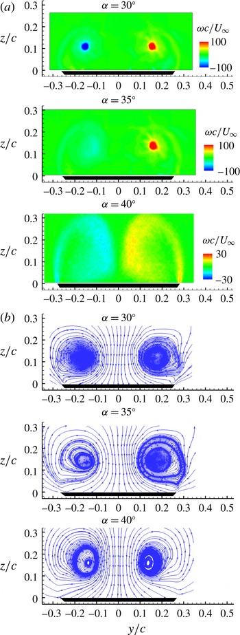
, one of the vortices exhibits breakdown while the other one does not, while the upstream (time-averaged) flow still seems symmetric. This different behaviour might be due to small imperfections in the geometry of the wing or small (undesired) yaw angle of the model. For the largest angle of attack, both vortices exhibit breakdown. However, for all three angles of attack, the time-averaged flow does not display any great asymmetry. In fact, the corresponding streamline patterns shown in figure 4(b) reveal roughly symmetric flow patterns. Even in the case of breakdown of both vortices when the distributed vorticity patches become closer to each other, there is no significant asymmetry in the time-averaged flow.
Time-averaged vorticity over the delta wing with
 $\unicode[STIX]{x1D6EC}=75^{\circ }$
at various chordwise locations: (a)
 $\unicode[STIX]{x1D6FC}=30^{\circ }$
; (b)
 $\unicode[STIX]{x1D6FC}=40^{\circ }$
.
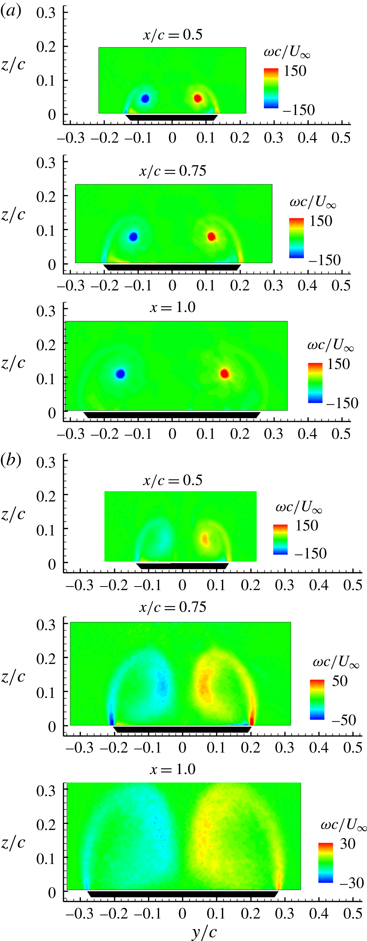
Time-averaged flow at
 $x/c=1.0$
for the delta wing with
 $\unicode[STIX]{x1D6EC}=75^{\circ }$
: (a) vorticity; (b) streamlines.

Vorticity distributions for the
 $80^{\circ }$
sweep wing are presented in figure 5 where the vortex pair appears to be symmetric and without any breakdown for
 $\unicode[STIX]{x1D6FC}=35^{\circ }$
. For
 $\unicode[STIX]{x1D6FC}=40^{\circ }$
, the vortices at the station
 $x/c=0.5$
have no breakdown. Further downstream both vortices exhibit breakdown, however the vortex pairs appear roughly symmetric. For the
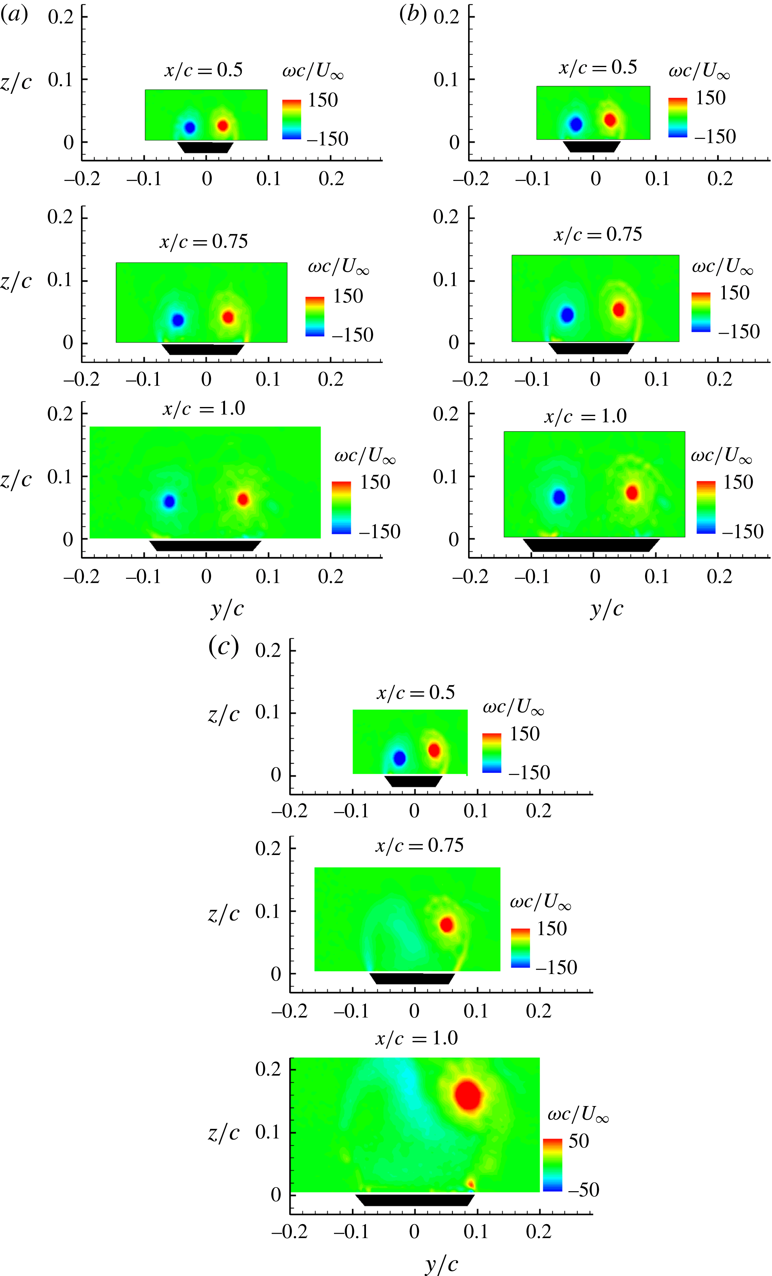
 $85^{\circ }$
sweep wing, however, the situation is different as shown in figure 6. Although the vortex pair is symmetric (within the experimental uncertainty) at lower angles of attack (
 $\unicode[STIX]{x1D6FC}\leqslant 25^{\circ }$
, not shown here), slight asymmetry at all three measurement planes can be seen from the vorticity plots at
 $\unicode[STIX]{x1D6FC}=30^{\circ }$
, without any vortex breakdown, as shown in figure 6(a). The asymmetry level grows with increasing angle of attack to
 $\unicode[STIX]{x1D6FC}=35^{\circ }$
, again without any breakdown. At the largest angle of attack, the first measurement plane shows increased asymmetry. Further downstream one of the vortices undergoes breakdown. It is clear that vortex asymmetry can develop well upstream of breakdown and also in the absence of breakdown on the wing.
Time-averaged vorticity over the delta wing with
 $\unicode[STIX]{x1D6EC}=80^{\circ }$
at various chordwise locations: (a)
 $\unicode[STIX]{x1D6FC}=35^{\circ }$
; (b)
 $\unicode[STIX]{x1D6FC}=40^{\circ }$
.

Time-averaged vorticity over the delta wing with
 $\unicode[STIX]{x1D6EC}=85^{\circ }$
at various chordwise locations: (a)
 $\unicode[STIX]{x1D6FC}=30^{\circ }$
; (b)
 $\unicode[STIX]{x1D6FC}=35^{\circ }$
; (c)
 $\unicode[STIX]{x1D6FC}=40^{\circ }$
.

3.2 Effect of the similarity parameter
 $K$

The vortex location, vortex strength and vortex core radius have been extracted for all three wings and are shown as a function of
 $K$
in figures 7–13. In doing so we have excluded all measurements with vortex breakdown (even if only one of the vortices had breakdown). We have not tried to determine the exact location of vortex breakdown on the wing, rather decided whether the breakdown occurred upstream or not. In the cases with breakdown, both the size of the vortices and magnitude of the axial velocity are significantly (almost one order of magnitude) different from those of the cases without breakdown. The spanwise
 $y_{v}$
and normal
 $z_{v}$
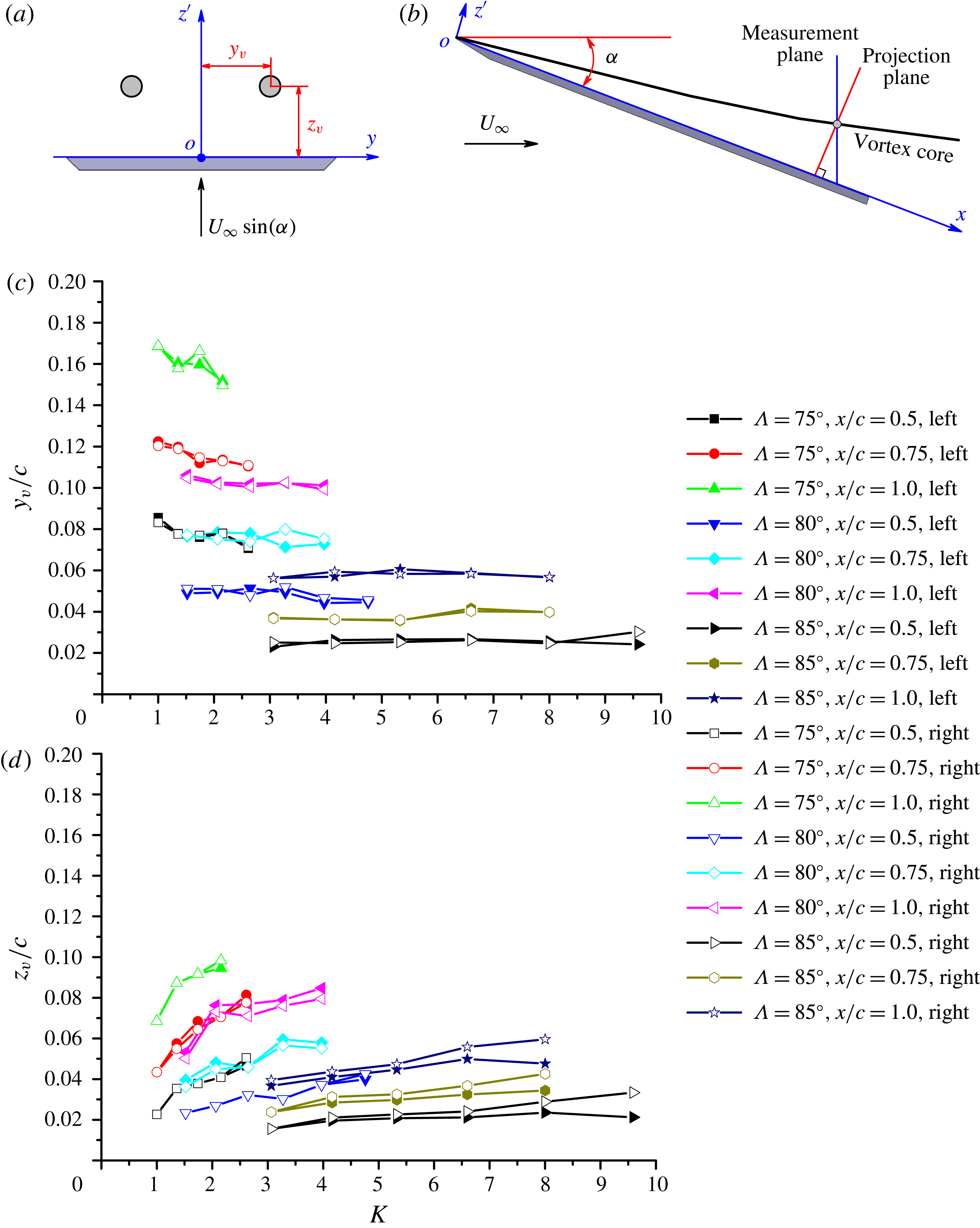
coordinates of the vortices are defined in figure 7(a), and the positions are identified by the maximum vorticity within the vortex cores. It should be noted that the normal position of vortices is defined in the plane perpendicular to the wing surface (chordwise axis
 $x$
), thus the normal positions calculated need to be projected into the plane from the measurement plane, as shown in figure 7(b), but the spanwise coordinates do not need any projection. Figure 7(c,d) shows the variation of the vortex locations with the similarity parameter
 $K$
, in which the coordinates are non-dimensionalized by the chord length
 $c$
. For these experiments, the chord length
 $c$
is the same for all three wings, therefore the variation of vortex locations in figure 7(c,d) can also be viewed as absolute magnitudes. It is seen that the vortices move upwards and outboard as the chordwise distance is increased. Increasing sweep angle results in vortex pairs becoming closer to the wing and moving inboard. There is not much difference between the left and right vortices in figure 7(c), however there is growing asymmetry in the normal coordinate (see figure 7
d) at large values of
 $K$
.
Vortex location versus similarity parameter
 $K$
: (a) definition of vortex location; (b) projection of normal location of vortices from measurement plane; (c) spanwise location
 $y_{v}/c$
against
 $K$
; (d) normal location
 $z_{v}/c$
against
 $K$
.

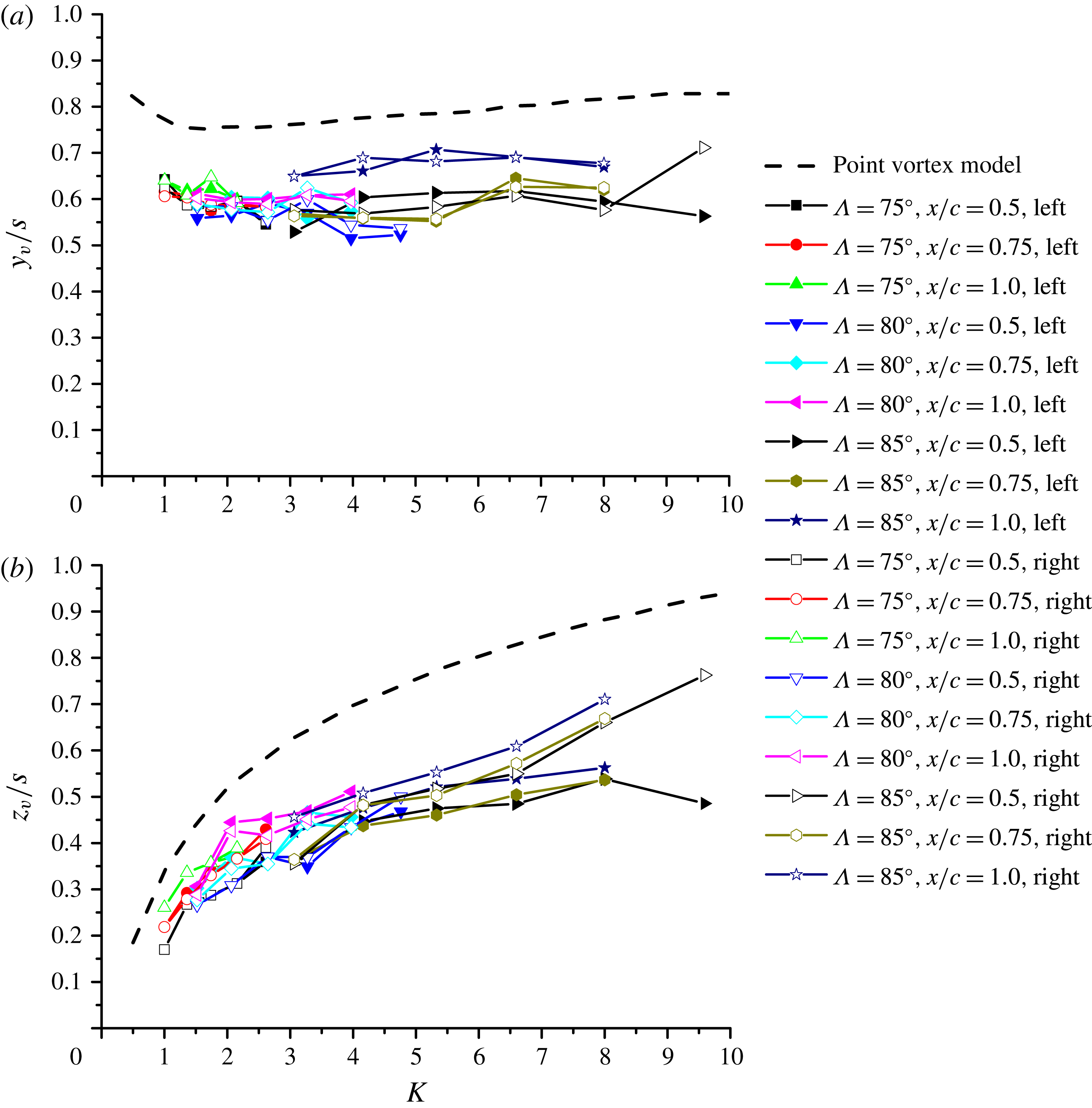
Vortex location non-dimensionalized by local semi-span
 $s$
as a function of
 $K$
: (a) spanwise location
 $y_{v}/s$
against
 $K$
; (b) normal location
 $z_{v}/s$
against
 $K$
.

Ratio of vortex spanwise location to normal location
 $y_{v}/z_{v}$
as a function of
 $K$
.

(a) Difference in the normal locations of vortices normalized by the core radius as a function of
 $K$
; (b) decomposition of total vorticity into the symmetric and antisymmetric vorticity for the largest
 $K$
; (c) variation of normalized integrated enstrophy as a function of
 $K$
.

Variation of circulation around each vortex in vortex pair with angle of attack for the wing with
 $\unicode[STIX]{x1D6EC}=75^{\circ }$
: (a) non-dimensional circulation based on chord length
 $c$
and free stream velocity
 $U_{\infty }$
; (b) non-dimensional circulation based on chord length
 $c$
and cross-flow component of free stream velocity
 $U_{\infty }\sin \unicode[STIX]{x1D6FC}$
.

Variation of circulation around each vortex with
 $K$
for all three wings: (a) non-dimensional circulation based on chord length
 $c$
and cross-flow component of free stream velocity
 $U_{\infty }\sin \unicode[STIX]{x1D6FC}$
; (b) non-dimensional circulation based on local semi-span length
 $s$
and cross-flow component of free stream velocity
 $U_{\infty }\sin \unicode[STIX]{x1D6FC}$
.

Variation of vortex core radius with
 $K$
for all three wings: (a) non-dimensional vortex radius based on local semi-span length
 $s$
; (b) non-dimensional vortex radius based on separation distance
 $b$
between the vortices.

Figure 8 presents the non-dimensional vortex location based on local semi-span
 $s$
, in which the data at various measurement planes collapse well. The results clearly indicate that the flows around slender delta wings exhibit the characteristics of conical flow. The spanwise coordinate of the vortices
 $y_{v}/s$
is basically unchanged with increasing
 $K$
, but the normal coordinate
 $z_{v}/s$
increases continuously with increasing
 $K$
. Theoretical vortex locations from a point-vortex model based on the slender-body theory are also provided as a comparison (Cai, Liu & Luo Reference Cai, Liu and Luo2001). The trends for the theoretical and experimental variations agree well, however the theory overestimates the vortex locations, i.e. vortices are more outboard and further away from the wing than the experiments. In addition, the spanwise
 $y_{v}/s$
and normal coordinate
 $z_{v}/s$
for the left and right vortices start to exhibit differences at higher
 $K$
values, indicating the development of vortex asymmetry.
The ratio of
 $y_{v}$
to
 $z_{v}$
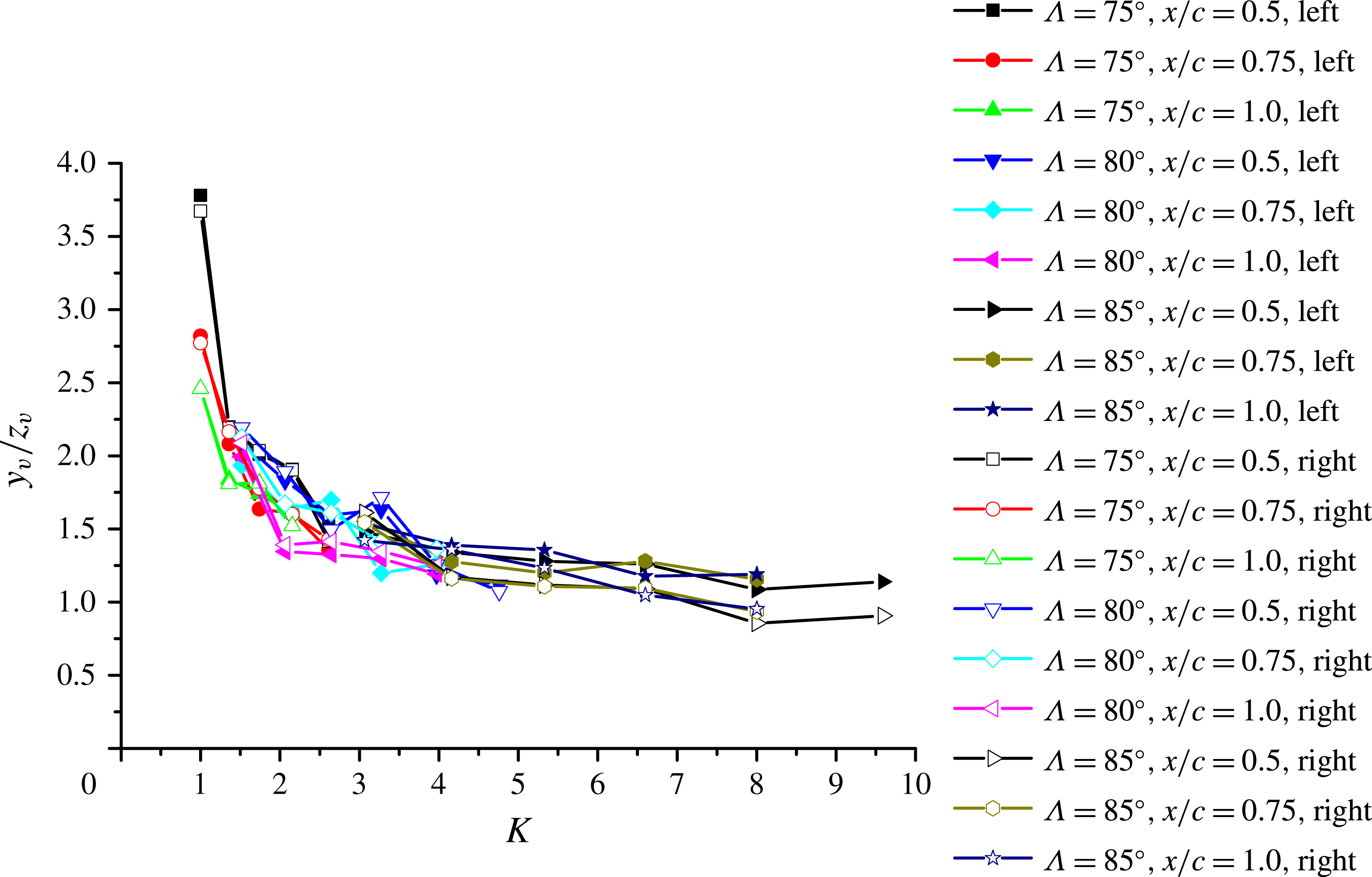
, which can be interpreted as the ratio of the vortex separation to the distance from the ‘image’ vortex, is shown in figure 9. It is seen that two vortices are gradually becoming closer to each other relative to their normal height as
 $K$
increases. The equilibrium location of the vortices is the result of the combined effects of the image vortices, the vortex sheets separated from the wing (which are usually much weaker than the concentrated vortices) as well as the flow due to the normal component of the free stream velocity. Figure 10(a) shows one of the most important observations of this paper. The difference in the normal coordinates of the two vortices increases with increasing
 $K$
, indicating that the vortex pair gradually becomes asymmetric. Obviously, it is impossible to have a perfectly symmetric model in the laboratory, however the important point is that small imperfections have no effect for low values of the similarity parameter
 $K$
and that the vortex pair is still symmetric. With increasing value of
 $K$
(only the
 $85^{\circ }$
sweep angle wing has sufficiently large values of
 $K$
), a small imperfection might have favoured the right vortex moving up. While for a perfectly symmetrical model, the left vortex moving up is as likely, this has not been tested by repeated settings of the wings. It is noted again that the data shown in figure 10 include only the vortex pairs with no breakdown, although vortex breakdown may be on the wing and upstream of the measurement plane in some cases. Apparently this does not create any asymmetry for
 $\unicode[STIX]{x1D6EC}=75^{\circ }$
and
 $80^{\circ }$
wings. For
 $\unicode[STIX]{x1D6EC}=85^{\circ }$
, vortex breakdown is on the wing and upstream of the measurement plane for one value (largest value) of
 $K$
only, and the onset of the asymmetry starts at smaller values of
 $K$
when there is no breakdown.
In figure 10(a), the vortex asymmetry is normalized by the vortex core radius
 $a$
. The vortex radius
 $a$
was obtained by using integration of the second-order moment of vorticity inside vortex cores (Leweke et al.
Reference Leweke, Le Dizés and Williamson2016) in order to take into account the non-axisymmetry of the vorticity distribution. There are 9–19 data points in the core radius, depending on the measurement plane. The ‘noise’ for the low values of
 $K$
is due to the spatial resolution of the PIV data. Based on the suggestion of an anonymous reviewer, we split the total vorticity into symmetric and antisymmetric parts. An example is shown in figure 10(b) for the largest
 $K$
value. The symmetric vorticity part represents the asymmetry of the vortex pair. This is different from the case of merging vortices of the same sign, where the asymmetric vorticity represents the asymmetry parameter (Cerretelli & Williamson Reference Cerretelli and Williamson2003). In order to calculate the amplitude of the asymmetric field, we squared the symmetric part of the vorticity (enstrophy) and integrated over the measurement plane:
 $E_{vort}=\int 0.5^{\ast }\unicode[STIX]{x1D714}_{s}^{2}\,\text{d}y\,\text{d}z$
. This was made dimensionless, taking into account the conical nature of the flow:
 $E_{vort}^{\ast }=E_{vort}/((U_{\infty }^{2}/c^{2})s^{2})$
where
 $s$
is the local semi-span. This was plotted as a function of
 $K$
in figure 10(c). Similarly, the kinetic energy of the asymmetric part of the velocity field can be integrated and plotted in the dimensionless form, which gives very similar results. It is seen that the ‘noise’ at low values of
 $K$
is eliminated, however the main conclusion of increasing asymmetry with increasing
 $K$
remains the same.
We now return to discussion of the properties of the time-averaged vortex pairs. Variation of the circulation of the vortices is shown in figures 11 and 12. It would be desirable to compare measured circulation with that of the point-vortex model in which the wing surface is normal to the cross-flow component
 $U_{\infty }\sin \unicode[STIX]{x1D6FC}$
according to the slender-body theory (Cai et al.
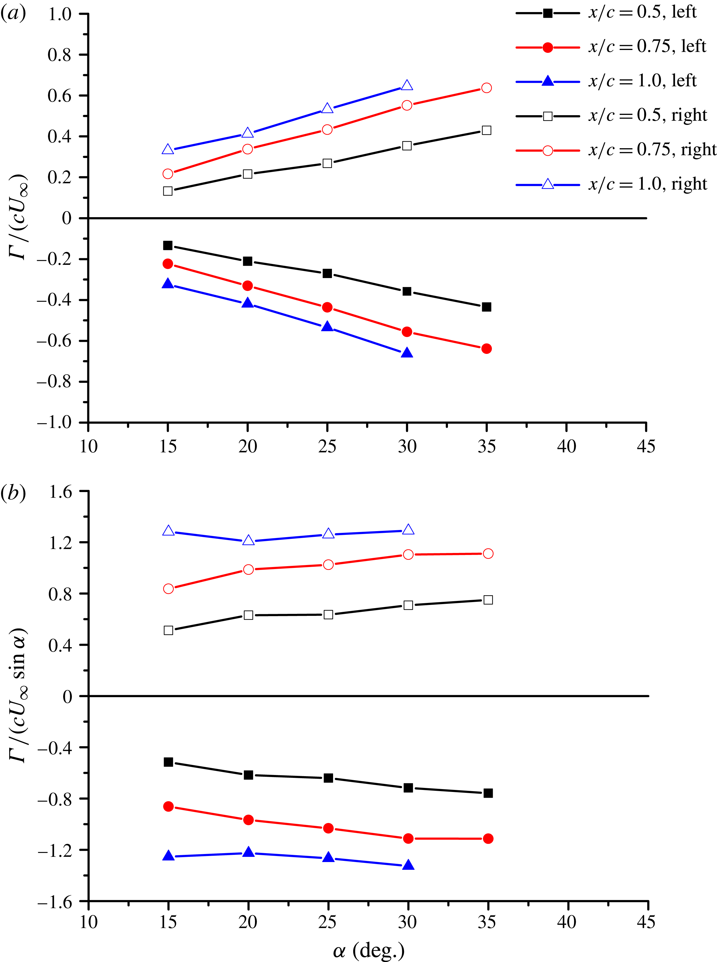
Reference Cai, Liu and Luo2003). However, our PIV measurement plane is not perpendicular to the wing surface, but normal to the free stream direction. The calculation of circulation in inclined planes to the vortex axis will not introduce an error according to the first Helmholtz theorem (Wu, Ma & Zhou Reference Wu, Ma and Zhou2006). Figure 11(a) shows that, for the
 $\unicode[STIX]{x1D6EC}=75^{\circ }$
wing, the circulation increases almost linearly with increasing angle of attack. Again, data with vortex breakdown have been excluded. If the normal component of the free stream speed
 $U_{\infty }\sin \unicode[STIX]{x1D6FC}$
is taken as the characteristic velocity (see the sketch in figure 7
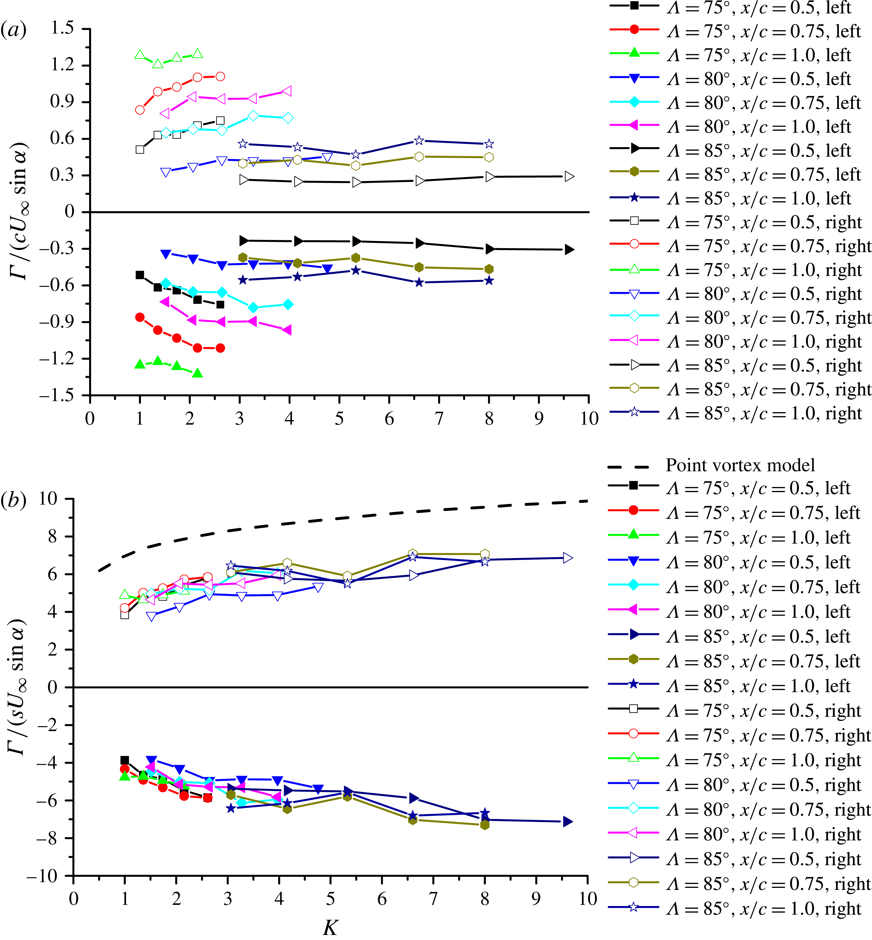
a), the effect of angle of attack can be eliminated, and the non-dimensional circulation is roughly constant with varying angle of attack, as shown in figure 11(b). Figure 12(a) shows the variation of the non-dimensional circulation as a function of
 $K$
, for all wings. It is seen that the circulation decreases with increasing
 $K$
, but the data are scattered owing to the effect of the chordwise distance at different measurement planes. This can be taken into account by the conical-flow assumption. Non-dimensional circulation based on the semi-span and the cross-flow component of the free stream velocity
 $U_{\infty }\sin \unicode[STIX]{x1D6FC}$
collapses well, and is a function of the similarity parameter
 $K$
only, as shown in figure 12(b). The theoretical prediction from the point-vortex model (Cai et al.
Reference Cai, Liu and Luo2001) is also included, and shown with the dashed line. It is seen that the theoretical circulation is significantly higher than the experimental values, although the trend is similar. In summary, circulations and vortex locations used in previous studies of the stability of point-vortex pairs are significantly different from the experimental measurements. This may be important for more realistic stability calculations.
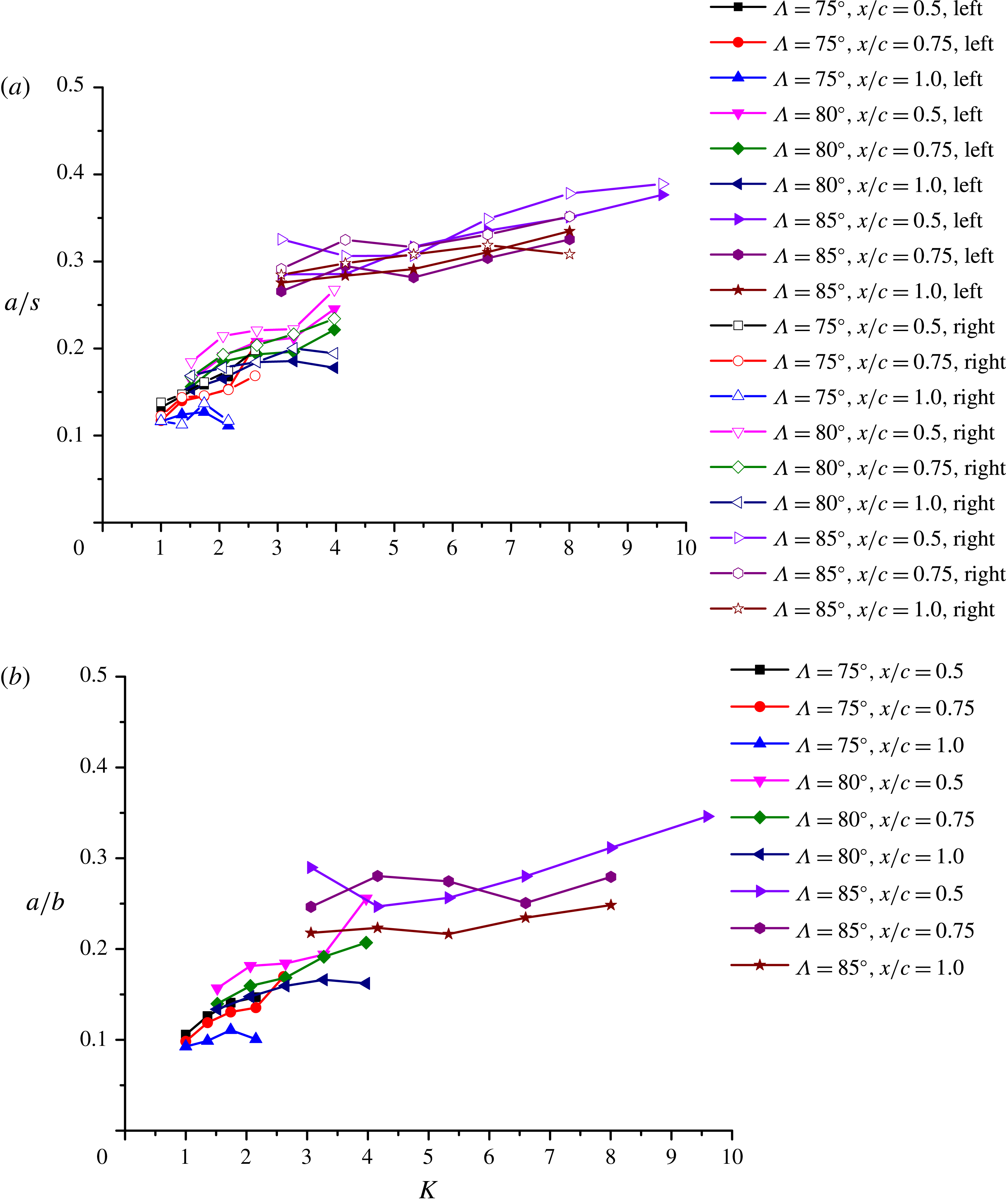
Finally, we discuss the variation of vortex core radius. The core radius determined from the time-averaged flow field grows almost linearly in the conical flow. When normalized by the local semi-span, which varies linearly with the chordwise distance, the ratio
 $a/s$
is nearly constant at different measurement planes as shown in figure 13(a). This is, in fact, the evidence that the conical-flow assumption is valid. The vortex radius normalized by the local semi-span shows reasonable collapse of the data with the parameter
 $K$
, and increases with increasing
 $K$
(figure 13
a). There seems to be a jump in the normalized radius between
 $K=3$
and 4 for the
 $\unicode[STIX]{x1D6EC}=85^{\circ }$
wing, suggesting that the most slender wing produces relatively larger vortex cores. Finite vortex core size might be important for more realistic stability calculations. Global instability analysis (Theofilis Reference Theofilis2011) of conical vortex pairs with realistic, non-axisymmetric vortices under the influence of the pressure gradient set by the wing may be useful in the near future.
Due to the vortex meandering (or wandering), the instantaneous core radius will always be smaller than that determined from the time-averaged flow field. The difference between the two is typically small. Even for relatively large meandering amplitudes (
 $\unicode[STIX]{x1D70E}/a\approx 0.34$
), Devenport et al. (Reference Devenport, Rife, Liapis and Follin1996) finds an instantaneous core radius which is 12 % smaller. For comparison, we calculated the ensemble average of the vortex radius from the instantaneous flow fields. In this case, we used ‘the circulation method’ (Raffel et al.
Reference Raffel, Willert, Wereley and Kompenhans2007) for the instantaneous velocity fields to calculate the filtered vorticity and then found the second-order moment of vorticity. For the two extreme (smallest and largest) values of the similarity parameter
 $K$
, we found that the ensemble-averaged core radius is smaller than that of the time-averaged vortex as expected, but the difference reduces from 9 % to 2 % with increasing
 $K$
. Therefore, we continue to use the time-averaged properties.
The variation of
 $a/b$
is shown in figure 13(b) for all measurements as a function of
 $K$
. For long wavelength instability, the separation distance
 $b$
increases linearly for the conical flow. Hence a direct comparison with the parallel vortex pairs is not possible. For the short wavelength instability, the smallest calculated Reynolds number
 $\unicode[STIX]{x1D6E4}/\unicode[STIX]{x1D708}$
is around
 $1.3\times 10^{4}$
at the
 $x/c=1$
measurement plane in our experiments (for
 $\unicode[STIX]{x1D6EC}=85^{\circ }$
), however we again note that this quantity also increases linearly for a conical flow. In the next section, we examine the vortex instabilities by means of the proper orthogonal decomposition and the dynamic mode decomposition.
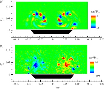
Main types of first POD modes: (a) shear layer instability for the wing of
 $\unicode[STIX]{x1D6EC}=85^{\circ }$
at
 $\unicode[STIX]{x1D6FC}=15^{\circ }$
and
 $x/c=0.75$
; (b) axisymmetric vortex mode for the wing of
 $\unicode[STIX]{x1D6EC}=75^{\circ }$
at
 $\unicode[STIX]{x1D6FC}=20^{\circ }$
and
 $x/c=0.5$
; (c) helical vortex mode for the wing of
 $\unicode[STIX]{x1D6EC}=80^{\circ }$
,
 $\unicode[STIX]{x1D6FC}=35^{\circ }$
,
 $x/c=1.0$
.

3.3 Flow instabilities
3.3.1 Overview
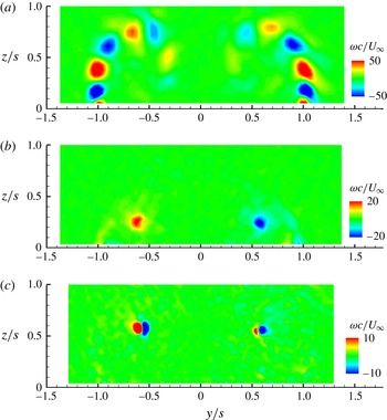
The proper orthogonal decomposition and dynamic mode decomposition analyses were carried out on instantaneous PIV snapshots for all measurement planes and wings. Figure 14 shows three typical examples of the first dominant modes observed for all wings in the absence of vortex breakdown. In general, the percentage of the total energy for first modes is small and energy is distributed over a large number of modes. For example, the energy percentages of the first modes are 5.7 % for (a), 4.5 % for (b) and 2.8 % for (c) in figure 14. The dominant mode in figure 14(a) represents the Kelvin–Helmholtz instability of the separated shear layers. As the instantaneous flow is the sum of the mean flow plus the POD modes (multiplied by some coefficients), the vorticity concentrations of alternating sign seen in this mode represent a decrease of total vorticity in one half of the wavelength and an increase in the other, resulting in instantaneous vorticity concentrations of the same sign in the shear layer. These small vortical substructures in the shear layers are generally dominant modes at lower angles of attack and for lower values of
 $K$
. The first mode shown in figure 14(b) represents oscillations of vorticity magnitude in the vortex cores, and can be considered as an axisymmetric mode (azimuthal wavenumber
 $m=0$
, Fabre, Sipp & Jacquin (Reference Fabre, Sipp and Jacquin2006). The first mode shown in figure 14(c) represents nearly vertical displacements. This leading POD mode, which is characterized by the vortex dipoles centred on the time-averaged vortex, has 2.8 % of the total energy. Higher modes not shown here have dipoles that are nearly orthogonal to those in figure 14(c). For example, for the left vortex, the next mode that is orthogonal has 1.5 % of the total energy. Even though the amplitudes of these two modes are not equal, the paired helical mode (with 1.5 % of the total energy) is still the most energetic mode. Therefore, these modes can be considered to be paired helical
 $m=1$
modes. This mode represents a helical displacement of the core, and was called the displacement wave by Fabre et al. (Reference Fabre, Sipp and Jacquin2006). Recently it was found for a tip vortex that the structure of the POD mode obtained experimentally and predicted by a spatial stability analysis of the mean flow agreed well (Edstrand et al.
Reference Edstrand, Davis, Schmid, Taira and Cattafesta2016). The helical mode was observed with wing tip vortices (Roy & Leweke Reference Roy and Leweke2008; Del Pino et al.
Reference Del Pino, Lopez-Alonso, Parras and Fernandez-Feria2011; Chen et al.
Reference Chen, Wang, Cleaver and Gursul2016), delta wing vortices (Zhang et al.
Reference Zhang, Wang and Gursul2016) and inlet/ground vortices (Wang & Gursul Reference Wang and Gursul2012). All these experimental observations showed that the dominant modes are orthogonal to each other. Amplification of the helical mode was also theoretically predicted by a transient energy growth analysis of the Lamb–Oseen vortex (Antkowiak & Brancher Reference Antkowiak and Brancher2004). It was shown that
 $m=1$
disturbances in the vortex can have transient amplification.
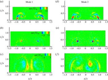
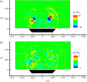
These three types of dominant mode in the absence of vortex breakdown exist simultaneously in many cases, although they are generally weak. Figure 15 shows the first two modes in the same measurement plane
 $(x/c=0.75)$
for the same wing
 $(\unicode[STIX]{x1D6EC}=75^{\circ })$
as the angle of attack is increased: (a)
 $\unicode[STIX]{x1D6FC}=20^{\circ }$
, (b)
 $\unicode[STIX]{x1D6FC}=30^{\circ }$
, (c)
 $\unicode[STIX]{x1D6FC}=40^{\circ }$
. Figure 15(a,d) shows the Kelvin–Helmholtz instability mode and the vortex helical mode in the first dominant mode (2 % of the total energy) and the second dominant mode (1.7 % of the total energy). Figure 15(b,e) shows the vortex axisymmetric mode (mode 1, 2.2 % of the total energy) and the vortex helical mode (mode 2, 0.5 % of the total energy) together with a very weak shear layer instability. Finally, in figure 15(c,f), we show the first (4.3 % of the total energy) and the second (3 % of the total energy) dominant modes in the presence of vortex breakdown.
Variation of the first two POD modes with angle of attack for the wing of
 $\unicode[STIX]{x1D6EC}=75^{\circ }$
at
 $x/c=0.75$
((a–c) show POD mode 1 and (d–f) show POD mode 2): (a,d)
 $\unicode[STIX]{x1D6FC}=20^{\circ }$
; (b,e)
 $\unicode[STIX]{x1D6FC}=30^{\circ }$
; (c,f)
 $\unicode[STIX]{x1D6FC}=40^{\circ }$
.

Some of the modes shown in figures 14 and 15 are symmetric while the others are antisymmetric. However, instantaneous flow is made of many modes which are relatively weak, and there is overall weak correlation between the left and right vortex cores. For the most slender wing
 $\unicode[STIX]{x1D6EC}=85^{\circ }$
at
 $\unicode[STIX]{x1D6FC}=30^{\circ }$
, we found a correlation coefficient of
 $R\approx 0.15$
at
 $x/c=0.5$
between the vorticity fluctuations in the left and right vortex cores. When the measurement plane was moved downstream to
 $x/c=1.0$
, the correlation coefficient was still small, but with the opposite sign,
 $R\approx -0.2$
. Therefore, we do not have strong evidence of the vortex-pair instabilities which would suggest significant correlation between the vortices, regardless of whether the time-averaged vortices are symmetric or not. Likewise, the spanwise and normal velocity components in the vortex cores are weakly correlated. Therefore, we do not have evidence of vortex-pair displacements as modelled by the temporal stability analysis of the point-vortex pairs (Huang & Chow Reference Huang and Chow1996; Cai et al.
Reference Cai, Liu and Luo2003). In the next section, we examine the quasi-periodicity of the flow instabilities.
3.3.2 Shear layer instabilities
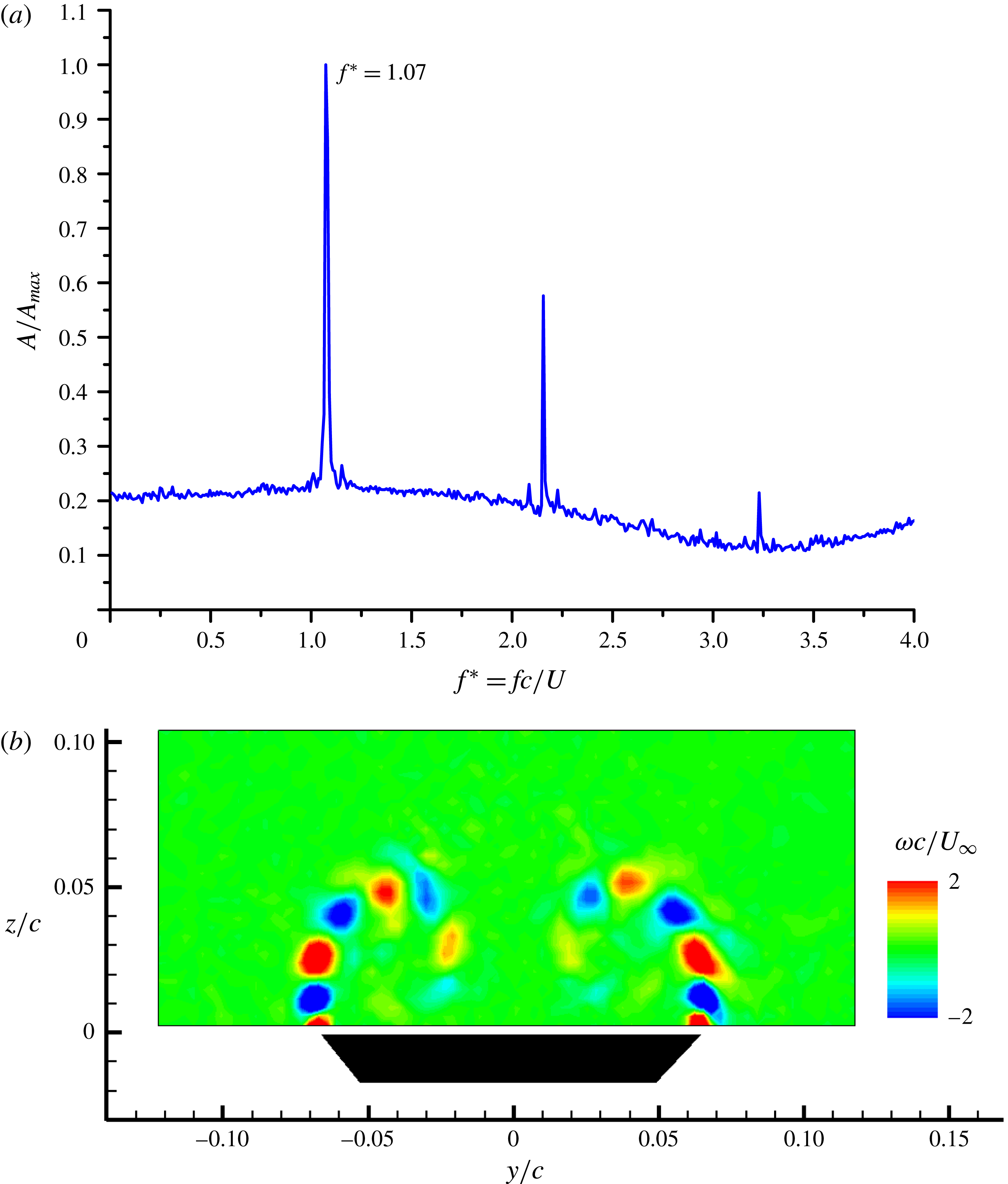
The Kelvin–Helmholtz instability had the most quasi-periodic nature compared to the other instabilities. Figure 16 shows the results of the dynamic mode decomposition analysis for
 $\unicode[STIX]{x1D6EC}=85^{\circ }$
,
 $\unicode[STIX]{x1D6FC}=15^{\circ }$
, at
 $x/c=0.75$
. The frequency spectrum of the amplitude shows a dominant frequency at
 $fc/U_{\infty }=1.07$
and its higher harmonics. Figure 16(b) shows the dominant DMD mode corresponding to the dominant frequency. This mode is very similar to the POD mode shown in figure 14(a) for the same measurement plane. Hence, the most energetic mode is also the most periodic mode.
(a) Frequency spectrum of the DMD modes, (b) dominant DMD mode for the wing of
 $\unicode[STIX]{x1D6EC}=85^{\circ }$
at
 $\unicode[STIX]{x1D6FC}=15^{\circ }$
and
 $x/c=0.75$
.

For the same wing and angle of attack, figure 17(a) shows the dominant DMD mode further downstream near the trailing edge,
 $x/c=1.0$
. This mode is very similar to the one shown in figure 16(b) for
 $x/c=0.75$
. Figure 17(b) shows an instantaneous vorticity field at
 $x/c=1.0$
, which reveals the vortical substructures in the shear layer which wraps around the vortex. The spacing (wavelength) of the vortices is consistent with the DMD mode in figure 17(a). These instantaneous vortical substructures do not show any evidence of vortex pairing around the primary vortex. Although we do not see any evidence of organized smaller-scale structures in the measurement window, initial development of the shear layer near the leading edge might involve higher-frequency vortical substructures and pairing as found by Gad-el-Hak & Blackwelder (Reference Gad-el-Hak and Blackwelder1985). The spacing (wavelength) of the vortices in the DMD modes in figure 17(a) and figure 16(b) is similar. In fact, the dominant frequency in the two planes is very similar:
 $fc/U_{\infty }=1.07$
and 1.10. Also, in the most upstream plane we found
 $fc/U_{\infty }=1.07$
. Considering that the measurements in different planes are not simultaneous, we can say that the dominant shear layer frequency is approximately constant in the chordwise direction. This finding is similar to the observations of Gad-el-Hak & Blackwelder (Reference Gad-el-Hak and Blackwelder1985) for non-slender delta wings with
 $\unicode[STIX]{x1D6EC}=45^{\circ }$
and
 $60^{\circ }$
.
(a) Dominant DMD mode, (b) instantaneous vorticity for the wing of
 $\unicode[STIX]{x1D6EC}=85^{\circ }$
at
 $\unicode[STIX]{x1D6FC}=15^{\circ }$
and
 $x/c=1.0$
.

Direct numerical simulations (Gordnier & Visbal Reference Gordnier and Visbal1994) clearly show that the shear layer frequency decreases almost linearly with the chordwise distance. As the perfectly conical geometry is used in the simulations, this result may be due to the small-scale vortices being attached to the apex. The experiments of Gad-el-Hak & Blackwelder (Reference Gad-el-Hak and Blackwelder1985) suggest constant frequency in the chordwise direction, although their wings had much lower sweep angles. We found that, even for high sweep angles, the shear layer frequency does not vary with downstream distance. This implies that the apex of the wing cannot keep the vortices pinned in the experiments, perhaps due to its finite size no matter how small it is.
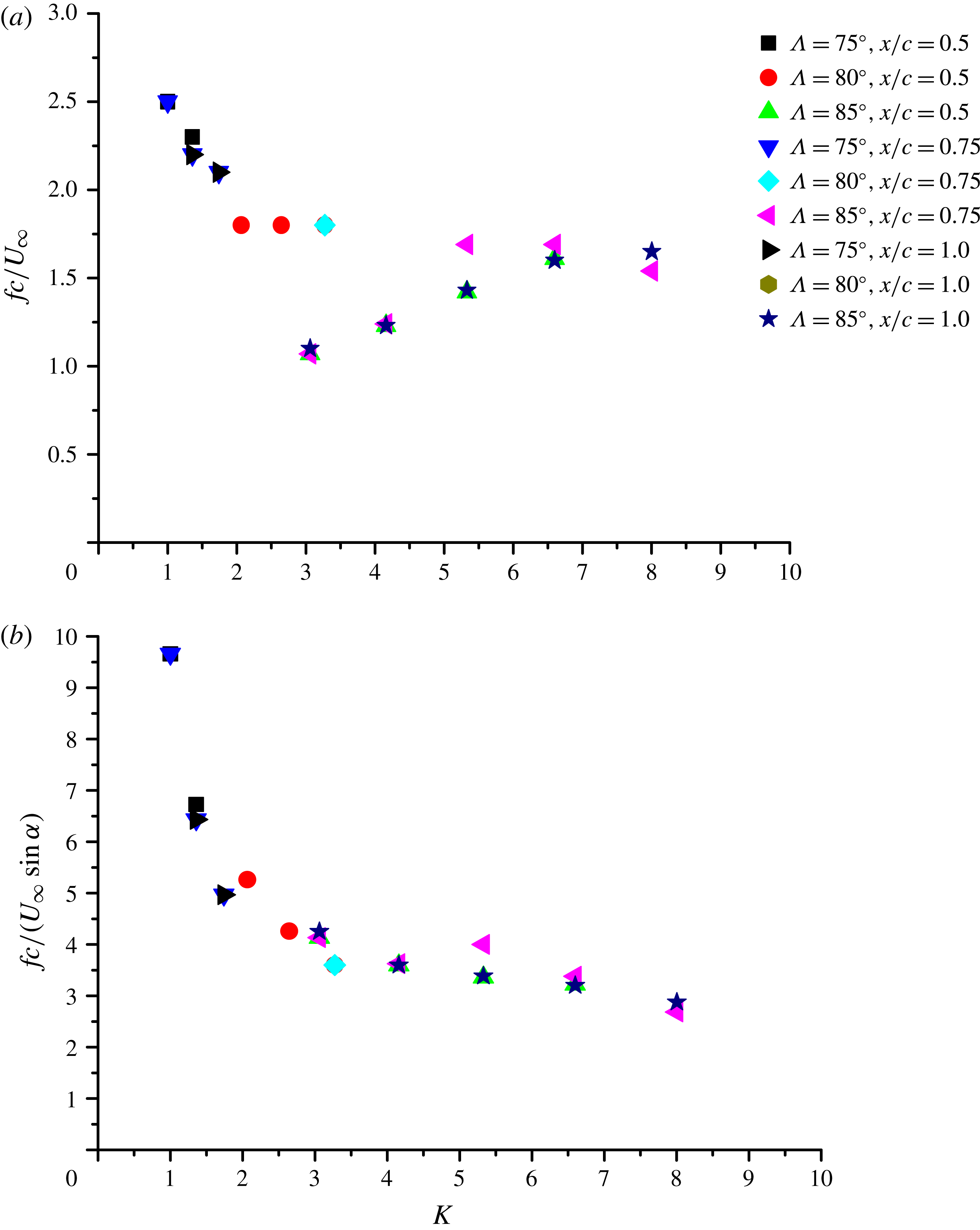
As the frequency does not show a dependency characteristic of conical flow, we plot
 $fc/U_{\infty }$
(rather than
 $fs/U_{\infty }$
) for all wings and measurement planes as a function of
 $K$
in figure 18(a). The scatter of the data may be caused by the fact that the characteristic velocity is not the free stream velocity. Gordnier & Visbal (Reference Gordnier and Visbal1994) showed that linear stability analysis of the mixing layer in the cross-flow plane could predict the shedding frequency successfully. Such a two-dimensional flow approach in the cross-flow plane suggests that the characteristic velocity in the definition of the Strouhal number might be the normal component of the free stream velocity,
 $U_{\infty }\sin \unicode[STIX]{x1D6FC}$
. Figure 18(b) shows the variation of
 $fc/(U_{\infty }\sin \unicode[STIX]{x1D6FC})$
as a function of
 $K$
. The data show excellent collapse, confirming the appropriate choice of the variables.
Variation of dominant frequencies of shear layer instability with
 $K$
, obtained by DMD: (a) non-dimensional frequency based on chord length
 $c$
and free stream velocity
 $U_{\infty }$
; (b) non-dimensional frequency based on chord length
 $c$
and cross-flow component of free stream velocity
 $U_{\infty }\sin \unicode[STIX]{x1D6FC}$
.

(a) First POD mode, (b) first DMD mode for the wing of
 $\unicode[STIX]{x1D6EC}=85^{\circ }$
at
 $\unicode[STIX]{x1D6FC}=35^{\circ }$
and
 $x/c=0.75$
.

The Strouhal numbers reported in figure 18(a) appear to be smaller than those reported in the experiments (
 $\unicode[STIX]{x1D6EC}=45^{\circ }$
,
 $60^{\circ }$
,
 $Re=1.2\times 10^{4}{-}3.3\times 10^{5}$
, Gad-el-Hak & Blackwelder Reference Gad-el-Hak and Blackwelder1985) and numerical simulations (
 $\unicode[STIX]{x1D6EC}=76^{\circ }$
,
 $Re=5\times 10^{4}$
, Gordnier & Visbal Reference Gordnier and Visbal1994). The reasons for this discrepancy are unknown. One possible reason might be the number of vortex pairings in the initial shear layer near the leading-edge region. Gordnier & Visbal (Reference Gordnier and Visbal1994) report no vortex pairing (in the absence of an external excitation in the simulations), while Gad-el-Hak & Blackwelder (Reference Gad-el-Hak and Blackwelder1985) report vortex pairing ‘at least three times’. We only see large vortical substructures around the main vortex, with no pairing in the flow fields at the current spatial resolution of the measurements.
3.3.3 Vortex instabilities
When the most energetic modes revealed axisymmetric or helical vortex instabilities, we did not find much periodicity of the flow. For example, figure 19 shows the first POD mode (5.6 % of the total energy) and the first DMD mode (which is a weak shear layer mode) for
 $\unicode[STIX]{x1D6EC}=85^{\circ }$
,
 $\unicode[STIX]{x1D6FC}=35^{\circ }$
, at
 $x/c=0.75$
. The frequency spectrum of the DMD analysis (not shown here) was noisy and the largest amplitude (at
 $fc/U_{\infty }=1.54$
) was 60 % higher than the background noise. Lack of periodicity in the helical mode can be understood in terms of the expected frequency/wavelength of this instability. Various experiments in wing tip vortices (Roy & Leweke Reference Roy and Leweke2008; Del Pino et al.
Reference Del Pino, Lopez-Alonso, Parras and Fernandez-Feria2011) and ground vortices (Wang & Gursul Reference Wang and Gursul2012) suggest that this helical mode has a long wavelength in the range
 $\unicode[STIX]{x1D706}/a=O(10^{2})$
to
 $O(10^{3})$
. Such long wavelength displacements were explained by the transient growth of the perturbations of azimuthal wavenumber
 $m=1$
in the Lamb–Oseen vortex without axial flow (Antkowiak & Brancher Reference Antkowiak and Brancher2004; Pradeep & Hussain Reference Pradeep and Hussain2006). Antkowiak and Brancher numerically simulated the transient growth of the
 $m=1$
mode, but also discussed the mechanism of growth in the limit of infinitely large wavelength. They showed that initial spiral disturbances develop into a vortex dipole quickly in the two-dimensional case and substantial transient growth exists. Heaton & Peake (Reference Heaton and Peake2007) revealed that the growth becomes infinite as the wavelength becomes very large for the helical mode. The applicability of the transient growth analysis for very large wavelengths remains an open question, however previous experimental findings suggest the existence of helical waves of large wavelength. Heaton & Peake (Reference Heaton and Peake2007) showed that the effect of axial flow in the core does not change the main conclusion that largest growth still occurs as
 $ka\rightarrow 0$
. Recently, Edstrand et al. (Reference Edstrand, Davis, Schmid, Taira and Cattafesta2016) performed a spatial stability analysis of a Batchelor vortex and found the same
 $m=1$
helical mode with very large wavelength as in their velocity measurements of a tip vortex. Therefore, we expect this mode to occur at very low frequencies. We do not, of course, know whether the helical waves are the result of an inherent instability or transient amplification of external noise. If we assume
 $a/c=O(10^{-1})$
(based on figure 13) and
 $\unicode[STIX]{x1D706}/a=O(10^{3})$
, we estimate
 $\unicode[STIX]{x1D706}/c=O(10^{2})$
, which implies
 $fc/U_{\infty }=O(10^{-2})$
. In our experiments, the smallest frequency that could be resolved was
 $fc/U_{\infty }\approx 0.01$
and we did not detect any periodicity of the vortex modes. It is likely that there might be some periodicity at longer wavelengths (smaller frequencies), which would require even longer durations of data acquisition.
As discussed previously there is not much correlation between the vortices when the time-averaged vortex pair is symmetric. The helical mode instability develops independently in each vortex. This is also true when symmetry breaking (in the time-averaged sense) takes place such as in figure 19. In fact, in the cases where one vortex had breakdown and the other did not, the helical mode instability could be detected in the unbroken vortex (for example,
 $\unicode[STIX]{x1D6EC}=85^{\circ }$
,
 $\unicode[STIX]{x1D6FC}=40^{\circ }$
, at
 $x/c=0.75$
and 1.00).
3.3.4 Vortex breakdown
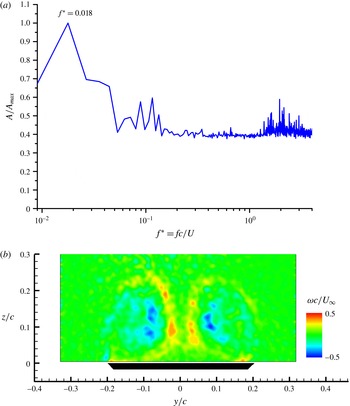
The DMD analysis showed that there are low-frequency oscillations when vortex breakdown exists on the wing. Figure 20 shows the spectrum and the dominant mode at
 $fc/U_{\infty }=0.018$
. Note that the dominant mode is a symmetric function of the spanwise coordinate
 $y$
. When this symmetric mode is added to the mean vorticity field, which is antisymmetric in the
 $y$
-direction, it represents an asymmetry in the magnitudes of vorticity of the left and right vortices. This could be caused by the antisymmetric oscillations of vortex breakdown locations, which are known to occur at low frequencies (Menke et al.
Reference Menke, Yang and Gursul1999).
(a) Frequency spectrum of the DMD modes, (b) dominant DMD mode for the wing of
 $\unicode[STIX]{x1D6EC}=75^{\circ }$
at
 $\unicode[STIX]{x1D6FC}=40^{\circ }$
and
 $x/c=0.75$
.

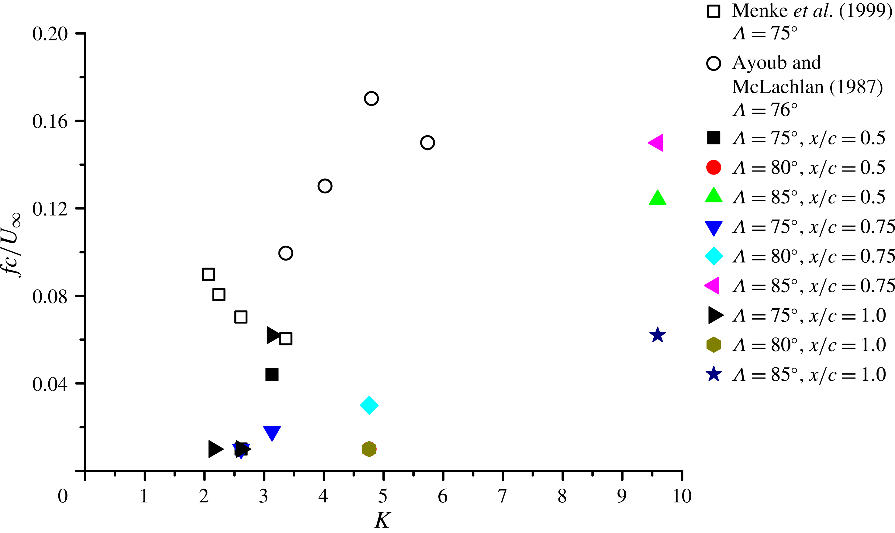
In figure 21, we plotted the Strouhal number of the low frequency oscillations as a function of
 $K$
. The solid symbols show our experiments (the DMD analysis results) for all wings when there is vortex breakdown. We also added the data points (with open symbols) obtained in other experiments (Menke et al.
Reference Menke, Yang and Gursul1999; Ayoub & McLachlan Reference Ayoub and McLachlan1987) by visualizing the locations of breakdowns. Overall, the orders of magnitude of the low-frequency oscillations are consistent, although the Strouhal number does not exhibit good collapse. In particular, the very low Reynolds number
 $(Re=2250)$
of Ayoub & McLachlan (Reference Ayoub and McLachlan1987) might have contributed to this scatter. Other forms of the Strouhal numbers did not provide better collapse of the data.
Variation of dominant frequency of vortex breakdown with
 $K$
.

4 Conclusions
An investigation of the symmetry breaking of conical vortex pairs over thin slender delta wings was carried out in a water tunnel using particle image velocimetry measurements. As the flow separation location at the leading edge is fixed, this geometry offers fundamental simplicity. It is shown that time-averaged vortex asymmetry can develop in the absence of vortex breakdown on the wing.
The vortex location in the cross-flow plane, vortex core radius and vortex strength data, which agree with the conical-flow assumptions, all collapse well when plotted as a function of the similarity parameter
 $K$
which combines the sweep angle and angle of attack. Experimentally measured vortices are located more inboard and closer to the wing surface, and are weaker in strength compared to the point vortex model used previously in the temporal stability calculations. It is shown that the asymmetry in the distance of the vortices from the wing increases gradually with increasing
 $K$
as the two vortices become closer to each other. Location, strength and finite core size of the vortices may be important for more realistic stability calculations. The axial velocity of the vortices has not been measured as this has not been possible with the current PIV system. However, even without any knowledge of the axial velocity excess, we observe the conical nature of the other vortex properties (location, circulation, core radius). In addition, the onset of the vortex asymmetry depends only on the similarity parameter. We note that the slender-body theory also neglects the axial velocity excess.
The asymmetric vortex flows on delta wings have been observed in previous investigations, but these limited observations have been complicated by the model geometry in some cases, where the apex region did not ensure ‘fixed separation’ points. On the other hand, even for fixed separation points, the observed asymmetry was attributed to vortex breakdown by some researchers whereas others observed no relation to vortex breakdown. While the experimental observations and interpretations have been contradictory, limited theoretical analysis using point vortices in conical flow and slender-body theory suggest that conical vortex pairs are always stable and should not exhibit any asymmetry. The present work not only shows that vortex asymmetry exists for fixed separation points, and unrelated to vortex breakdown, but also proposes a single parameter for its onset.
We have investigated the features of the instantaneous flow and found a very small correlation coefficient between the vorticity fluctuations in the centres of the vortices. Likewise, there has been no significant correlation between the velocities of the vortices in the cross-flow plane. We have been able to capture the shear layer modes and vortex modes (mostly axisymmetric and first helical modes) by using proper orthogonal decomposition analysis, however the modes are weak. The total energy is distributed over many modes. The shear layer mode is also the most dominant in the dynamic mode decomposition analysis, particularly for lower values of
 $K$
. The dominant frequency of the shear layer mode does not have the conical flow characteristic. The Strouhal number
 $fc/(U_{\infty }\sin \unicode[STIX]{x1D6FC})$
is a function of the similarity parameter
 $K$
only. This choice of the characteristic velocity
 $U_{\infty }\sin \unicode[STIX]{x1D6FC}$
suggests that cross-flow analysis of the shear layer instability is appropriate. The helical vortex mode did not show much periodicity, and this could be caused by the very large wavelengths (very low frequencies) expected for this instability. On the other hand, low-frequency oscillations were detected in the presence of vortex breakdown, which agree with previous flow visualization studies of vortex breakdown.
Acknowledgements
The first author acknowledges financial support from the National Natural Science Foundation of China (NSFC) under grant no. 11272033.