3.1 Validation of the code

To validate the numerical approach, oscillatory flow over a plane and smooth wall, where a single sphere is kept fixed, was simulated for a value of the Reynolds number $R_{\unicode[STIX]{x1D6FF}}$ equal to $47.87$ . The dimensionless diameter $D=D^{\ast }/\unicode[STIX]{x1D6FF}^{\ast }$ of the sphere was set equal to $6.267$ and the sphere did not touch the bottom but its dimensionless distance $\unicode[STIX]{x1D716}=\unicode[STIX]{x1D716}^{\ast }/\unicode[STIX]{x1D6FF}^{\ast }$ from it was set equal to $0.0978$ , which is equal to the value used by Fischer et al. (Reference Fischer, Leaf and Restrepo2002). These values of the parameters were chosen to allow a comparison of the present results with those of Fischer et al. (Reference Fischer, Leaf and Restrepo2002). Figure 2 shows the spanwise vorticity component in a vertical plane aligned with the direction of the fluid oscillations and crossing the centre of the sphere. Different phases of the cycle are considered after the flow reaches a periodic state. The phases are chosen equal to those considered by Fischer et al. (Reference Fischer, Leaf and Restrepo2002) in their figure 3 and a qualitative comparison can be easily made. This comparison shows that the present approach provides a reliable description of the oscillatory flow around an object. Indeed, looking at figure 2 and at figure 3 of Fischer et al. (Reference Fischer, Leaf and Restrepo2002), it can be observed that counter-clockwise spanwise vorticity is generated along the sphere surface when the external flow moves from the right to the left of the figure. The production of counter-clockwise vorticity intensifies, when the clockwise vortex shed during the previous half-cycle is convected from the right to the left and travels above the top of the sphere. Then, the flow separates at the sphere crest and the free shear layer tends to be convected by the clockwise vortex which moves because dragged by the free stream flow. Later, further counter-clockwise vorticity is shed, which tends to roll up and to generate a counter-clockwise rotating vortex. Meanwhile, the clockwise rotating vortex, previously shed by the sphere surface, dissipates because of viscous effects. Then, the counter-clockwise rotating vortex is convected from the left to the right and the phenomenon repeats specularly during the following half-cycle.

Figure 2.

Spanwise component of the vorticity computed in the middle vertical plane crossing the sphere ( $x_{2}=30$ ) for $R_{\unicode[STIX]{x1D6FF}}=47.87$ , $D=6.267$ , $\unicode[STIX]{x1D716}=\unicode[STIX]{x1D716}^{\ast }/\unicode[STIX]{x1D6FF}^{\ast }=0.09777$ at $t=\unicode[STIX]{x1D714}^{\ast }t^{\ast }=3.66\unicode[STIX]{x03C0}$ , (a); $t=3.80\unicode[STIX]{x03C0}$ , (b); $t=3.96\unicode[STIX]{x03C0}$ , (c); $t=4.44\unicode[STIX]{x03C0}$ , (d); $t=4.50\unicode[STIX]{x03C0}$ , (e). The vorticity isolines are for $\unicode[STIX]{x1D714}_{2}^{\ast }\unicode[STIX]{x1D6FF}^{\ast }/U_{0}^{\ast }=\pm 0.2,\pm 0.5,\pm 1,\pm 2,\pm 3,\pm 4$ (solid lines $=$ positive values, broken lines $=$ negative values). When comparing the present results with those by Fischer et al. (Reference Fischer, Leaf and Restrepo2002), the reader should consider that the values of the vorticity isolines in Fischer et al.’s paper are unknown.

Figure 3.

Time development of the lift coefficient $C_{L}$ for a single sphere in an oscillatory boundary layer over a smooth wall for $R_{\unicode[STIX]{x1D6FF}}=47.87$ , $D=6.267$ and $\unicode[STIX]{x1D716}=\unicode[STIX]{x1D716}^{\ast }/\unicode[STIX]{x1D6FF}^{\ast }=0.09777$ . (a) Present results; (b) Fischer et al.’s Reference Fischer, Leaf and Restrepo2002 results.

Figure 4.

Streamwise velocity component at different phases of the cycle in the middle vertical plane crossing the largest sphere for $R_{\unicode[STIX]{x1D6FF}}=56$ , $D=28$ , $d=2.6$ and $\unicode[STIX]{x1D716}=0.374$ . The thin solid ( $u_{1}>0$ ) and broken ( $u_{1}<0$ ) lines are the isovelocity contours $(\unicode[STIX]{x0394}u_{1}=0.1)$ and the thick solid line corresponds to $u_{1}=0$ . (a) $t=\unicode[STIX]{x03C0}$ , (b) $t=9\unicode[STIX]{x03C0}/8$ , (c) $t=10\unicode[STIX]{x03C0}/8$ , (d) $t=11\unicode[STIX]{x03C0}/8$ , (e) $t=12\unicode[STIX]{x03C0}/8$ , (f) $t=13\unicode[STIX]{x03C0}/8$ , (g) $t=14\unicode[STIX]{x03C0}/8$ , (h) $t=15\unicode[STIX]{x03C0}/8$ . Particularly high-velocity regions in the wake of the sphere are denoted by the label A.

Figure 5.

Streamwise velocity component at $t=\unicode[STIX]{x03C0}$ , when the free stream velocity is maximum, in the region close to the bottom for $D=28$ , $d=2.6$ , $\unicode[STIX]{x1D716}=0.374$ and $R_{\unicode[STIX]{x1D6FF}}=56$ (a,c,e) and $R_{\unicode[STIX]{x1D6FF}}=112$ (b,d,f). (a,b) Region on the downstream side; (c,d) region on the upstream side and ( $e,f$ ) region far from the large sphere. The thin solid ( $u_{1}>0$ ) and broken ( $u_{1}<0$ ) lines are the isovelocity contours $(\unicode[STIX]{x0394}u_{1}=0.1)$ and the thick solid line corresponds to $u_{1}=0$ .

Figure 6.

Streamwise velocity component at different phases of the cycle in the horizontal plane crossing the largest sphere for $R_{\unicode[STIX]{x1D6FF}}=56$ , $D=28$ , $d=2.6$ and $\unicode[STIX]{x1D716}=0.374$ . The thin solid ( $u_{1}>0$ ) and broken ( $u_{1}<0$ ) lines are the isovelocity contours $(\unicode[STIX]{x0394}u_{1}=0.1)$ and the thick solid line corresponds to $u_{1}=0$ . (a) $t=\unicode[STIX]{x03C0}$ , (b) $t=9\unicode[STIX]{x03C0}/8$ , (c) $t=10\unicode[STIX]{x03C0}/8$ , (d) $t=11\unicode[STIX]{x03C0}/8$ , (e) $t=12\unicode[STIX]{x03C0}/8$ , (f) $t=13\unicode[STIX]{x03C0}/8$ , (g) $t=14\unicode[STIX]{x03C0}/8$ , (h) $t=15\unicode[STIX]{x03C0}/8$ . Regions of high velocity are denoted by B and C in panels (a) and (b).

Figure 7.

Detail of panel $(f)$ of figure 6 (red box). The computational grid is overlapped to contour patches (two confining mesh refinements can be seen). See the caption of figure 6 for the values of the simulation parameters.

No quantitative comparison can be made between the vorticity computed by means of the present code and that described by Fischer et al. (Reference Fischer, Leaf and Restrepo2002), because Fischer et al. (Reference Fischer, Leaf and Restrepo2002) do not provide the values of the isovorticity lines. A quantitative estimate of the accuracy of the present results can be made by comparing the time development of the lift coefficient $C_{L}$ plotted in figure 3 with that drawn in figure 3 of Fischer et al. (Reference Fischer, Leaf and Restrepo2002). Herein, the lift coefficient is defined as the ratio between the lift force and the quantity $(1/8)\unicode[STIX]{x1D70C}^{\ast }\unicode[STIX]{x03C0}D^{\ast 2}U_{0}^{\ast 2}$ . The agreement turns out to be fair (the largest difference is a few per cent of the maximum value) and similar to that observed comparing the velocity profiles with those obtained by Fischer et al. (Reference Fischer, Leaf and Restrepo2002).

3.2 The velocity field

Once the reliability of the code was ascertained, results were obtained by considering a large sphere over a rough bed made by much smaller spheres. The first simulation is characterized by $R_{\unicode[STIX]{x1D6FF}}=56.0,D=28.0$ and $d=2.6$ . Moreover, because of the numerical approach, the spheres do not touch the bottom but are $0.374\unicode[STIX]{x1D6FF}^{\ast }$ from it and are laid in a hexagonal arrangement. The distance of the spheres from the bottom, which is required for numerical reasons, is larger than that used in the previous run because small values of $\unicode[STIX]{x1D716}^{\ast }$ imply large computational costs and the value of $\unicode[STIX]{x1D716}^{\ast }$ does not affect significantly the flow above the roughness elements. Indeed, the results of Fornarelli & Vittori (Reference Fornarelli and Vittori2009) and those of Mazzuoli & Vittori (Reference Mazzuoli and Vittori2016), who computed the oscillatory flow above semi-spheres and spheres, respectively, show that the geometry of the wall roughness below the sphere centres does not affect significantly the flow above them. Figure 4 shows the value of the streamwise velocity component plotted in the vertical midplane aligned with the direction of the fluid oscillations, at different phases of the cycle starting from $\unicode[STIX]{x03C0}$ to $15\unicode[STIX]{x03C0}/8$ every $\unicode[STIX]{x03C0}/8$ , once the flow field attained a periodic state. As expected, the presence of the large sphere slows down the fluid in front of the sphere, while a recirculating region appears behind it. Moreover, high velocities are present just above the crest of the sphere. A careful analysis of the figure shows the presence of further high velocity regions in the wake of the sphere, the most evident of which is denoted by the label A in the figure. These regions, which are close to the bottom (see and compare figure 4 b–e), move and suggest the existence of vortex structures which are convected by the oscillating fluid and feel the effects of the self-induced velocity due to the interaction of the vortices with their image vortices below the seafloor. These vortex structures survive for a significant time interval as it can be inferred by the presence of regions (the most evident of which is denoted by A in figure 4 h) characterized by a positive velocity, while the fluid far from the bottom has a significant negative velocity.

The smaller spheres act as a bottom roughness and create a layer of fluid, the thickness of which is $O(d)$ , where the velocity almost vanishes. To show the details of the flow around the small spheres, the left-hand side panels of figure 5 show enlargements of the region close to the bottom, when the free stream velocity is positive and maximum. Near the large sphere, on the downstream side (see figure 5 a), the streamwise velocity component close to the bottom is directed from the right to the left while the free stream velocity is in the opposite direction. The flow reverses its direction because of the clockwise vorticity shed by the large sphere which induces negative velocities close to the bottom. On the other hand, on the upstream side (see figure 5 c), the velocity is positive but it assumes small values because of the blockage effect due to the resting large sphere. However, around the base of the sphere, the fluid accelerates and the streamwise velocity increases because the pressure on the stoss side of the sphere is larger than the pressure on the lee side. At last, far from the sphere (see figure 5 e), the velocity field is ‘homogeneous’ in the streamwise and spanwise directions. In particular, within the gaps among the small spheres, the fluid is practically at rest and significant velocities are observed only above the crests of the spheres. Figure 5 (right-hand side panels) also shows results for the same values of the parameters but for $R_{\unicode[STIX]{x1D6FF}}=112$ , which are discussed later on.

Figure 6 shows again the streamwise velocity component, at the same phases of the cycle as those considered in figure 4, but in a horizontal plane which crosses the centre of the large sphere. As expected, on the upstream side, the fluid slows down when approaching the sphere because of its blockage effect, while on the lateral sides it accelerates and the flow separates from the sphere surface along the downstream side, generating recirculating regions behind the sphere. Moreover, the presence of intense vortex structures shed by the sphere can be inferred by the regions of high velocity denoted by B and C in figure 6(a,b).

Some of the panels of figure 6 show very small flow structures which might appear not fully resolved. To show that the numerical grid is small enough to provide an accurate description of the time development of the flow field, figure 7 shows an enlargement of the region highlighted in figure 6(f), where the numerical grid is also plotted. Figure 7 shows that the grid size is much smaller than the smallest flow structures and it is small enough to provide reliable description of the viscous boundary layer which develops on the sphere surface (more quantitative results which support this statement are described later when larger values of the Reynolds number are considered such that smaller vortices are generated).

The flow described by figures 4–6 is practically the mirror image of that observed during the previous and following half-cycles. This finding, along with the symmetry of the flow with respect to the vertical plane crossing the centre of the large sphere and aligned with the flow direction, suggests that the flow is not turbulent. However, the signal of the velocity just behind the large sphere (see figure 8) shows that rapid fluctuations of the velocity are superimposed on much slower oscillations. The former are induced by the passage of the vortex structures shed by the large sphere while the latter are due to the oscillating pressure gradient which forces the fluid motion.

Since it is expected that an increase of the Reynolds number leads to stronger nonlinear effects and causes the generation of a larger number of vortex structures of smaller size, it might be that a chaotic flow appears and/or turbulence is triggered when the Reynolds number is increased. Indeed, Blondeaux & Vittori (Reference Blondeaux and Vittori1991) and Vittori & Blondeaux (Reference Vittori and Blondeaux1993), who investigated the two-dimensional oscillatory flow above a rippled bed and around a circular cylinder, respectively, found that the nonlinear interaction of coherent vortex structures gives rise to a chaotic flow when the Reynolds number becomes larger than a critical value.

Figure 8.

(a) Streamwise, (b) wall-normal and (c) spanwise components of the velocity at $(x_{1},x_{3})=(123.67,14.39)$ plotted versus time for $R_{\unicode[STIX]{x1D6FF}}=56$ , $D=28$ , $d=2.6$ , $\unicode[STIX]{x1D716}=0.374$ and $x_{2}=54.83$ (—○—), $x_{2}=61.83$ (—▫—), $x_{2}=68.83$ (—▵—).

Figure 9.

Streamwise velocity component at different phases of the cycle in the middle vertical plane crossing the largest sphere for $R_{\unicode[STIX]{x1D6FF}}=112$ , $D=28$ , $d=2.6$ and $\unicode[STIX]{x1D716}=0.374$ . The thin solid ( $u_{1}>0$ ) and broken ( $u_{1}<0$ ) lines are the isovelocity contours $(\unicode[STIX]{x0394}u_{1}=0.1)$ and the thick solid line corresponds to $u_{1}=0$ . (a) $t=\unicode[STIX]{x03C0}$ , (b) $t=9\unicode[STIX]{x03C0}/8$ , (c) $t=10\unicode[STIX]{x03C0}/8$ , (d) $t=11\unicode[STIX]{x03C0}/8$ , (e) $t=12\unicode[STIX]{x03C0}/8$ , (f) $t=13\unicode[STIX]{x03C0}/8$ , (g) $t=14\unicode[STIX]{x03C0}/8$ , (h) $t=15\unicode[STIX]{x03C0}/8$ . Particularly high-velocity regions in the wake of the sphere are denoted by the label A.

Figure 10.

(a) Streamwise, (b) wall-normal and (c) spanwise components of the velocity plotted versus time. $x_{1}=123.67$ , $x_{3}=14.39$ and $x_{2}=54.83$ (—○—), $x_{2}=61.83$ (—▫—), $x_{2}=68.83$ (—▵—). $R_{\unicode[STIX]{x1D6FF}}=112$ , $D=28$ , $d=2.6$ , $\unicode[STIX]{x1D716}=0.374$ .

To ascertain whether an increase of the Reynolds number leads to a turbulent flow, a further run was made for the same values of the parameters ( $D=28$ , $d=2.6$ , $\unicode[STIX]{x1D716}=0.374$ ) but for $R_{\unicode[STIX]{x1D6FF}}=112$ and figure 9, which is similar to figure 4, shows the streamwise velocity component. Since the dimensionless diameters of large and small spheres are kept fixed, the increase of Reynolds number is due to a proportional increase of $U_{0}^{\ast }$ . It follows that the Keulegan–Carpenter number of the phenomenon, $K_{c}=U_{0}^{\ast }/(\unicode[STIX]{x1D714}^{\ast }D^{\ast })$ , increases too and this explains why the streamwise size of computational box was increased.

The results show that the vortex structures, which are generated during each half-cycle by the roll up of the shear layer shed by the surface of the large sphere, break and generate an ensemble of small vortices on the lee side of the sphere. The nonlinear self-interaction of the small vortices in the wake of the large sphere gives rise to a turbulent flow, as it appears from figure 10 where the time development of the three velocity components just behind the sphere is plotted. Indeed, the rapid velocity fluctuations, which are superimposed on the slow oscillations induced by the pressure gradient, turn out to have a random character. Moreover, the velocity field is no longer the mirror image of the velocity fields which are observed during the following or previous half-cycles and the instantaneous flow field loses its symmetry with respect to the vertical plane which crosses the centre of the sphere and is aligned with the direction of the fluid oscillations.

The results of the numerical simulation for $R_{\unicode[STIX]{x1D6FF}}=112$ show that the flow in the wake of the large sphere is turbulent but the evaluation of turbulence characteristics is not simple. First of all, the flow induced by the forcing pressure gradient is oscillating and turbulence characteristics are time dependent and confined within relatively small regions. Moreover, the turbulent fluctuations are neither homogeneous nor isotropic.

In principle, the average flow field could be evaluated by using a phase average procedure and by taking advantage of some symmetries of the problem. However, the large computational costs did not allow us to simulate the flow for a large number of cycles. Since turbulence is observed in the wake of the sphere within relatively small regions, where turbulence characteristics weakly depend on the horizontal coordinates but they strongly vary in the vertical direction, we evaluate the velocity fluctuations $(u_{1}^{\prime },u_{2}^{\prime },u_{3}^{\prime })$ by subtracting a spatial averaged flow field $(\overline{u}_{1},\overline{u}_{2},\overline{u}_{3})$ from the actual values of the velocity field. The spatial average is performed over a volume which extends in the horizontal directions, covering the region where turbulence is detected, but it is quite thin, having a thickness equal to a few grid cells. Moreover, the turbulent velocity fluctuations are evaluated only at particular phases of the oscillatory cycle and far from the sphere, when and where turbulence can be assumed to be independent on the horizontal coordinates. In particular, the regions close to the sphere, where the coherent vortices shed by the sphere make turbulence characteristics to depend on $x_{1}$ and $x_{2}$ are not considered.

Then, the normalized two-point correlations of the velocity fluctuations are evaluated in the streamwise and spanwise directions. The results allow one to gain an estimate of the size of the vortex structures which characterize the turbulence field. For example, the normalized two-point correlation $R_{11}=\overline{u_{1}^{\prime }(\boldsymbol{x})u_{1}^{\prime }(\boldsymbol{x}+\boldsymbol{r})}/\overline{u_{1}^{\prime }(\boldsymbol{x})u_{1}^{\prime }(\boldsymbol{x})}$ is plotted at $(x_{1},x_{2},x_{3})=(276.33,47.64,16.63)$ as a function of $r_{1}$ and $r_{2}$ in figure 11. The results allow an estimate of (i) the longitudinal and lateral integral length scales of the turbulent fluctuations, which turn out to be of order $10\unicode[STIX]{x1D6FF}^{\ast }$ , and (ii) longitudinal and lateral Taylor microscales, which turn out to be of order $\unicode[STIX]{x1D6FF}^{\ast }$ . It is worth pointing out that the evaluation of $R_{11}$ was not made for larger values of $r$ , even though its value does not vanish for $r=22$ , because turbulence is present only in a small spatial region such that the evaluation of $R_{11}$ for larger values of $r$ would be meaningless. At last, the dissipation rate $\unicode[STIX]{x1D700}^{\ast }=\overline{(\unicode[STIX]{x2202}u_{i}^{\ast }/\unicode[STIX]{x2202}x_{j}^{\ast })(\unicode[STIX]{x2202}u_{i}^{\ast }/\unicode[STIX]{x2202}x_{j}^{\ast })}$ is evaluated again at $t=5.13\unicode[STIX]{x03C0}$ and it shows that the Kolmogorov scale $(\unicode[STIX]{x1D708}^{\ast 3}/\unicode[STIX]{x1D700}^{\ast })^{1/4}$ is of order $10^{-1}\unicode[STIX]{x1D6FF}^{\ast }$ , thus indicating that the grid size is sufficiently small to provide reliable results on turbulence dynamics.

Figure 11.

Normalized correlation function $R_{11}$ of the fluctuations of the streamwise velocity component, as a function of the streamwise and spanwise separations $r_{1}$ and $r_{2}$ , respectively, obtained at $t=5.13$ considering a rectangular volume centred in $(x_{1},x_{2},x_{3})=(276.33,47.64,16.63)$ of dimensions $(46.71\times 46.71\times 1.87)$ for $R_{\unicode[STIX]{x1D6FF}}=112$ , $D=28$ , $d=2.6$ .

Turbulence is generated also close to the rough bottom by the interaction of the large-scale coherent vortices, convected by the free stream, with the roughness elements (the small spherical particles). The results show that in this region the velocity fluctuations are highly anisotropic.

Even though turbulence is present in the wake of the large sphere, the bottom boundary layer (see figure 5 f) and the flow close to the large sphere (see figure 5 b) keep in the laminar regime. Indeed, no random oscillations of the velocity field are present above the small spheres as long as they do not interact with the vortices originated from the large sphere (see figure 5 f). This finding is in agreement with the results of Mazzuoli & Vittori (Reference Mazzuoli and Vittori2016) who observed that larger values of the Reynolds number are necessary to trigger turbulence appearance in the oscillatory boundary layer over spherical particles of similar size. For example, Mazzuoli & Vittori (Reference Mazzuoli and Vittori2016) found that the critical value of the Reynolds number for $d=2.32$ (a value which is close to $d=2.6$ ) ranges above $500$ .

Figure 12.

Spanwise component of the vorticity computed in the middle vertical plane (a,c,e,g,i) and vertical component of the vorticity computed in the horizontal plane crossing the centre of the sphere (b,d,f,h,j) for $R_{\unicode[STIX]{x1D6FF}}=56$ , $D=28$ , $d=2.6$ and $\unicode[STIX]{x1D716}=0.374$ at $t=21/8\unicode[STIX]{x03C0}$ , (a,b); $t=23/8\unicode[STIX]{x03C0}$ , (c,d); $t=25/8\unicode[STIX]{x03C0}$ , (e,f); $t=28/8\unicode[STIX]{x03C0}$ , (g,h); $t=4\unicode[STIX]{x03C0}$ , (i,j). The vorticity isolines are equispaced by $\unicode[STIX]{x0394}\unicode[STIX]{x1D714}_{2}=0.1$ in the range $\pm 0.8$ . Instead of the isoline $\unicode[STIX]{x1D714}_{2}=0$ , the value $\unicode[STIX]{x1D714}_{2}=-0.05$ is considered (solid lines $=$ positive values, broken lines $=$ negative values). A and B in panel (c) denote regions of high vorticity.

Figure 13.

Spanwise component of the vorticity computed in the plane $x_{2}=x_{2c}+20$ ( $x_{2c}$ being the spanwise coordinate of the centre of the large sphere) for $R_{\unicode[STIX]{x1D6FF}}=56$ , $D=28$ , $d=2.6$ and $\unicode[STIX]{x1D716}=0.374$ at $t=21/8\unicode[STIX]{x03C0}$ , (a) and $t=25/8\unicode[STIX]{x03C0}$ , (b). The vorticity isolines are equispaced by $\unicode[STIX]{x0394}\unicode[STIX]{x1D714}_{2}=0.1$ in the range $\pm 0.8$ . Instead of the isoline $\unicode[STIX]{x1D714}_{2}=0$ , the value $\unicode[STIX]{x1D714}_{2}=-0.05$ is considered (solid lines $=$ positive values, broken lines $=$ negative values).

Figure 14.

Streamwise component of the vorticity computed (a,b) in the middle vertical plane crossing the sphere centre $x_{1}=x_{1c}=95.66$ , (c,d) at $x_{1}=x_{1c}+0.5D$ and (e,f) at $x_{1}=x_{1c}+1.5D$ for $D=28$ , $d=2.6$ , $\unicode[STIX]{x1D716}=0.374$ , $t=\unicode[STIX]{x1D714}^{\ast }t^{\ast }=3\unicode[STIX]{x03C0}$ . (a,c,e), $R_{\unicode[STIX]{x1D6FF}}=56$ and (b,d,f), $R_{\unicode[STIX]{x1D6FF}}=112$ . The vorticity isolines are equispaced by $\unicode[STIX]{x0394}\unicode[STIX]{x1D714}_{2}=0.1$ in the range $\pm 0.8$ . Instead of the isoline $\unicode[STIX]{x1D714}_{2}=0$ , the value $\unicode[STIX]{x1D714}_{2}=-0.05$ is considered (solid lines $=$ positive values, broken lines $=$ negative values).

3.3 The vorticity field and the dynamics of the vortex structures

As discussed in the introduction, one of the aims of the work is the identification of the coherent vortex structures shed by the large sphere and their influence on the forces exerted by the fluid on the sediment spherical particles resting on the bottom. Similarly to figure 2, figure 12 (left-hand side panels) shows the spanwise vorticity component in the middle vertical plane crossing the sphere ( $x_{2}=30$ ) and aligned with the direction of the fluid oscillations for $R_{\unicode[STIX]{x1D6FF}}=56$ , $D=28$ , $d=2.6$ and $\unicode[STIX]{x1D716}=0.374$ for a few phases of the cycle. The main differences between the results of figure 12 and those of figure 2 are due to the different diameter of the large sphere and the presence of the spherical roughness elements in the former case. The numerical simulation shows that clockwise vorticity is generated along the surface of the large sphere when the fluids moves from left to right (see figure 12 a,c,e). Moreover, the production of vorticity increases as the fluid velocity close to the sphere increases because of either the external pressure gradient or the interaction of the sphere with a coherent vortex structure. When the flow reverses its direction, no further clockwise vorticity is generated along the surface of the sphere (figure 12 i) but the counter-clockwise rotating vortices (see vortices A and B in figure 12 c) still moves from left to right because of their interaction with the seafloor (see figure 12 e,g). Figure 12 shows that significant vorticity is also shed close to the seafloor by the small spheres and a thick boundary layer is present close to the bottom.

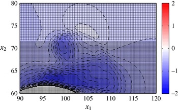
Up to now, the vorticity dynamics is discussed looking at the flow in a vertical plane crossing the centre of the large sphere and aligned with the direction of the fluid oscillations. However, the flow is not two-dimensional. Indeed, the vorticity is more intense around the large sphere on the lateral sides where a strong interaction of the vortex structures shed by the sphere takes place with the bottom roughness. In particular, figure 13 shows that the local deceleration of the external flow induced close to the bottom by a coherent vortex causes the separation of the bottom boundary layer and a complex dynamics of the vorticity field. The three-dimensional features of the flow are clearly shown in figure 12 (right-hand side panels) where the vertical vorticity component in a horizontal plane crossing the centre of the large sphere is plotted. The vortex structures shed by the sphere during half-cycle have a size larger than that which can be guessed on the basis of the spanwise vorticity plots and they are characterized by a more complex dynamics. In particular, figure 12(b,d,h) show that complex vortex structures exist where clockwise and counter-clockwise vorticity strongly interact. These vortex structures move away from the sphere till they break and dissipate. Finally, figure 14 shows the streamwise vorticity component in three different vertical planes orthogonal to the direction of the fluid oscillations and in the wake of the sphere, when the free stream velocity is maximum ( $t=3\unicode[STIX]{x03C0}$ ). The first plane crosses the centre of the large sphere, the second is tangent to the sphere on the downstream side and the third is one diameter apart. The figure shows that two counter-rotating streamwise vortices are present behind the sphere, which are close to the bed and strongly interact with the seafloor. In particular the streamwise vortices, which are close to the seafloor when they are near the sphere, lift from the bed as they move away from the sphere.

Figure 15.

Spanwise component of the vorticity computed in the middle vertical plane (a,c,e,g,i) and vertical component of the vorticity computed in the horizontal plane crossing the centre of the sphere (b,d,f,h,j) for $R_{\unicode[STIX]{x1D6FF}}=112$ , $D=28$ , $d=2.6$ and $\unicode[STIX]{x1D716}=0.374$ at $t=21/8\unicode[STIX]{x03C0}$ , (a,b); $t=23/8\unicode[STIX]{x03C0}$ , (c,d); $t=25/8\unicode[STIX]{x03C0}$ , (e,f); $t=28/8\unicode[STIX]{x03C0}$ , (g,h); $t=4\unicode[STIX]{x03C0}$ , (i,j). The vorticity isolines are equispaced by $\unicode[STIX]{x0394}\unicode[STIX]{x1D714}_{2}=0.1$ and visualized in the range $\pm 0.8$ . Instead of the isoline $\unicode[STIX]{x1D714}_{2}=0$ , the value $\unicode[STIX]{x1D714}_{2}=-0.05$ is considered (solid lines $=$ positive values, broken lines $=$ negative values).

Figure 16.

(a) Spanwise component of the vorticity computed at $x_{3}=7.38$ inside the red box indicated in figure 15 $(d)$ . The computational grid is overlapped to the contour patches. (b) Energy spectrum $E(\unicode[STIX]{x1D705}_{2})$ of the flow field shown in panel $(a)$ (red line A–B) is plotted versus the spanwise wavenumber $k_{2}$ for $x_{1}=229.3$ .

Figure 17.

Vortex structures visualized by (red) the contour surfaces of $\unicode[STIX]{x1D706}_{2}=-0.1$ , for $D=28,d=2.6,R_{\unicode[STIX]{x1D6FF}}=56$ at (a)  $t=21\unicode[STIX]{x03C0}/8$ , (b)  $t=23\unicode[STIX]{x03C0}/8$ , (c)  $t=25\unicode[STIX]{x03C0}/8$ , (d)  $t=28\unicode[STIX]{x03C0}/8$ , (e)  $t=4\unicode[STIX]{x03C0}$ . The curved vortex structures that move away from the sphere are denoted by C in panel (c).

A similar vorticity dynamics is observed for the larger value of $R_{\unicode[STIX]{x1D6FF}}$ ( $R_{\unicode[STIX]{x1D6FF}}=112$ ), even though the vortex structures, shed by the large sphere and moving away from it, break earlier and give rise to smaller vortices (see figure 15 a–f). The size of the turbulent eddies appearing in figure 15 is quite small and the reader might question the reliability and accuracy of the results. To show that also in this case the flow is well resolved, figure 16(a) shows an enlargement of the region highlighted in figure 15(d) along with the numerical grid which appears to be small enough to provide reliable and accurate results. To quantitatively support this statement, the energy spectrum of the flow field shown in figure 16(a) is computed as a function of the spanwise wavenumber $\unicode[STIX]{x1D705}_{2}$ for $x_{1}=229.3$ and plotted in figure 16(b). The results show that the energy of the smallest resolved flow components is negligible. Since similar results are obtained for different values of $(x_{1},x_{3})$ and $t$ (not shown herein), it clearly appears that the flow field is well resolved.

Since the analysis of isosurfaces of the velocity and vorticity components provides a partial information on the coherent vortex structures and may be considered inadequate to detect vortices in an unsteady three-dimensional flow, we computed the eigenvalues of the symmetric tensor  $\overline{\unicode[STIX]{x1D63F}}^{2}+\overline{\unicode[STIX]{x1D734}}^{2}$ ( $\overline{\unicode[STIX]{x1D63F}}$ is the strain rate tensor and $\overline{\unicode[STIX]{x1D734}}$ is the spin tensor) and we considered the regions with two negative eigenvalues. Indeed, as discussed by Jeong & Hussain (Reference Jeong and Hussain1995), these regions correlate well with coherent vortex structures buried in a background vorticity field. Figure 17 visualizes the isosurface characterized by a negative value of $\unicode[STIX]{x1D706}_{2}$ , which is the second eigenvalue of the tensor $\overline{\unicode[STIX]{x1D63F}}^{2}+\overline{\unicode[STIX]{x1D734}}^{2}$ ( $\unicode[STIX]{x1D706}_{2}=-0.1$ ) at different phases of the cycle for $R_{\unicode[STIX]{x1D6FF}}=56$ . The results plotted in figure 17 allow to visualise the three-dimensional structure of the vorticity field and to gain a clear idea of its dynamics. In particular, at $t=21\unicode[STIX]{x03C0}/8$ (figure 17 a), the fluid moves from the right to the left and the roll up of the vorticity shed by the sphere generates two vortex structures at the base of the sphere which grow in time because of the continuous shedding of vorticity. Later, when the flow reverses its direction, these vortex structures no longer grow but are simply convected from the left to the right. In particular, when the vortex structures come close to the sphere, they strongly interact with it and induce the shedding of two new vortex structures which couple with the vortices previously released from the sphere and move away from the sphere because of the free stream flow and the self-induced velocity (see figure 17 b). Meanwhile, two further vortex structures are shed by the sphere while the vortices previously generated decay because of viscous effects and their interaction with the rough bottom (see figure 17 d). The vorticity dynamics during the following half-cycle is practically the mirror image of that previously described. It is interesting to point out that those, which appear as vortex structures generated by the roll up of vorticity of the same sign, are indeed generated by the strong interaction of vortex structures of different sign as it can be inferred by the results plotted in figure 12(d), where it appears clearly that the curved vortex structures which move away from the sphere (denoted as C in figure 17(c)) are due to both clockwise and counter-clockwise vorticity (see figure 12 d,f).

3.4 The bottom shear stress and the forces acting on bottom particles

The present investigation was also aimed at identifying the regions of the seafloor where the vortices shed by the larger sphere tend to set the sediments into motion and sweep them away. A simple analysis shows that the sediment particles start to move when the bed shear stress becomes larger than a critical value which depends on the parameter $\sqrt{(\unicode[STIX]{x1D70C}_{s}^{\ast }/\unicode[STIX]{x1D70C}^{\ast }-1)g^{\ast }d^{\ast 3}}/\unicode[STIX]{x1D708}^{\ast }$ , which is known as both the Galilei/Galileo number and the sediment Reynolds number. Hence, the shear stress just above the small spheres is evaluated as a function of time and figure 18 shows its streamwise component at different phases of the cycle for $D=28,d=2.6$ and $R_{\unicode[STIX]{x1D6FF}}=56$ . As expected, the numerical results show that the shear stress acting on the seafloor (far from the large sphere) attains its maximum value with a phase shift $\unicode[STIX]{x1D719}\simeq \unicode[STIX]{x03C0}/4$ with respect to the free stream velocity. Indeed, the flow regime in the bottom boundary layer keeps laminar for $R_{\unicode[STIX]{x1D6FF}}=56$ and even for $R_{\unicode[STIX]{x1D6FF}}=112$ . The spatial and temporal distribution of the shear stress feels the effects of the large sphere and the action of the vortices shed by the sphere itself. Indeed, the largest values of the shear stress are found around the sphere in the lateral regions where the velocity attains its maximum values, while behind the sphere, regions of relatively small values of the shear stress are observed because of the shadow effect of the sphere which creates a sheltered area characterized by a relatively small velocity. Moreover, the footprints of the coherent vortex structures shed by the sphere can be easily identified, since the coherent vortices induce locally relatively high velocities and hence high values of the shear stress.

For example, at $t=11.98$ , the maximum values of the bed shear stress are attained in the vicinity of the large sphere and into two layers, which leave the lateral surface of the sphere in the downstream direction, because of the local large velocities induced by the sphere presence and the flow separation. However, at $t=10.21$ , when the shear stress far from the sphere is relatively small because of the flow inversion, the regions characterized by the largest values of the shear stress are in the wake of the sphere and can be paired with the coherent vortices convected by the free stream.

Figure 18.

Shear stress acting on the plane $x_{3}=3.08$ , just above the crest of the small roughness elements, shadowed by colours for $D=28,d=2.6,R_{\unicode[STIX]{x1D6FF}}=56$ . From left to right and from top to bottom: $t=9.82$ , $t=10.21$ , $t=11.39$ , $t=11.98$ .

Figure 19.

Top view of the bottom areas where the small spheres could be potentially mobilized by the flow during certain phases of the oscillatory period, in which the Shields parameter $\unicode[STIX]{x1D703}_{max}$ exceeds $\unicode[STIX]{x1D703}_{crit}=0.05$ , for either the relative density of the spheres $s=1.025$ (grey areas) or $s=1.05$ (red/darker areas) and $D=28,d=2.6$ . The broken line indicates the projection of the large sphere equator (a)  $R_{\unicode[STIX]{x1D6FF}}=56$ and (b)  $R_{\unicode[STIX]{x1D6FF}}=112$ .

Finally, the region where the flow would be able to move the small spheres at any phase of the cycle is visualized in figure 19(a). This region is evaluated by computing the modulus of the shear stress at each phase and selecting its maximum value $\unicode[STIX]{x1D70F}_{max}^{\ast }$ , during the oscillatory cycle, at each location. Then, the maximum value of the Shields parameter $\unicode[STIX]{x1D703}_{max}$ is computed as $\unicode[STIX]{x1D703}_{max}=\unicode[STIX]{x1D70F}_{max}^{\ast }/(\unicode[STIX]{x1D70C}_{s}^{\ast }-\unicode[STIX]{x1D70C}^{\ast })g^{\ast }d^{\ast }$ and the region of the possible motion of the small spheres is assumed to be coincident with the area of the sea bottom where $\unicode[STIX]{x1D703}_{max}$ is larger than a critical value $\unicode[STIX]{x1D703}_{crit}$ . The value of $\unicode[STIX]{x1D703}_{crit}$ depends on the particle Reynolds number $R_{p}=\sqrt{(\unicode[STIX]{x1D70C}_{s}^{\ast }/\unicode[STIX]{x1D70C}^{\ast }-1)g^{\ast }d^{\ast 3}}/\unicode[STIX]{x1D708}^{\ast }$ and different empirical relationships are available into the literature to determine $\unicode[STIX]{x1D703}_{crit}$ . One of the most used is that of Brownlie (Reference Brownlie1981) which has been recently amended by Parker, Seminara & Solari (Reference Parker, Seminara and Solari2003) dividing its value by a factor $2$ . For small values of $R_{p}$ , the relationships provide large values of $\unicode[STIX]{x1D703}_{crit}$ . However, Soulsby, Whitehouse et al. (Reference Soulsby and Whitehouse1997) noticed that, even for small grain sizes, the value of $\unicode[STIX]{x1D703}_{crit}$ never exceeds $0.3$ . To take into account this experimental evidence, he proposed a new relationship. Because of the large uncertainty which affects the estimate of $\unicode[STIX]{x1D703}_{crit}$ , the results of figure 19 are obtained by using $\unicode[STIX]{x1D703}_{crit}=0.05$ which is a reasonable estimate for relatively large spherical particles.

Because of the relatively large size of the small spheres and the weakness of the oscillatory flow, the region of potential erosion around the large sphere is quantified by assuming that the small spheres are made by a relatively light material (e.g. polyethylene with a relative density $s=\unicode[STIX]{x1D70C}_{s}^{\ast }/\unicode[STIX]{x1D70C}^{\ast }$ equal to both $1.025$ and $1.05$ ).

As it could be guessed on the basis of the time development of the streamwise component of the bottom shear stress (see figure 18), the results plotted in figure 19(a) show that the small spheres, simulating the sediments around the ‘large’ spherical object, tend to be swept away mainly from the sides of the large sphere and along the trajectories of the coherent vortex structures shed by the object. The symmetry of the flow is not perfect because it would be necessary to simulate more cycles to have a fully periodic regime. For $R_{\unicode[STIX]{x1D6FF}}=56$ , the small spheres, which simulate the sediment grains, would move only for $s=1.025$ . Moreover, sediment transport would be observed only in the region surrounding the large sphere while the sediment grains far from it would be at rest (clear water conditions). On the other hand for $R_{\unicode[STIX]{x1D6FF}}=112$ and $s=1.025$ (see figure 19 b), the small spheres would move also far from the large sphere even though the largest values of the shear stress and the most intense sediment transport would be observed close to the large sphere. However, increasing $s$ ( $s=1.05$ ), the sediment motion would again be confined in the region close to the large sphere and clear water conditions would be observed.

Finally, we should point out that the critical value of the Shields parameter is evaluated on the basis of an empirical approach which is based on data obtained for steady flows and does not take into account the effects of the pressure gradient oscillations (Sleath Reference Sleath1999). Even though it is likely that the oscillatory character of the flow has no significant influence on the initiation of sediment motion because of the large ratio between the fluid displacement oscillations and the sediment size, future simulations with mobile particles might provide detail information on the conditions of incipient motion of sediment particles in oscillatory flows, which is still an active area of research (Frank et al. Reference Frank, Foster, Sou and Calantoni2015a ,Reference Frank, Foster, Sou, Calantoni and Chou b ).

Figure 20.

Top view of the lower part of the bottom layer of particles (a). Red (on the right) and blue (on the left) spheres are numerically instrumented to determine the hydrodynamic force exerted by the flow oscillations. The broken black line indicates the equator of the large sphere ( $R_{\unicode[STIX]{x1D6FF}}=112,D=28,d=2.6$ and five layers of small spheres arranged in a hexagonal patterns). Time development of the horizontal ( $\sqrt{F_{1}^{2}+F_{2}^{2}}$ ) (b) and vertical ( $F_{3}$ ) (c) components of the hydrodynamic force as well as the spanwise torque component ( $T_{2}$ ) (d) acting on the small spheres indicated in panel (a) (blue-cross and red-circle lines are related to the blue (left) and red (right) spheres, respectively) located either in the top layer [——] or in the bottom layer [- - -]. Panel (e) shows the velocity far from the bottom.

To better simulate the flow close to and within the sea bottom, the run for $D=28,d=2.6,R_{\unicode[STIX]{x1D6FF}}=112$ was repeated with five layers of sediment particles, laid over the plane rigid wall located at $x_{3}=0$ . If the results obtained for these values of the parameters are compared with those previously discussed, no qualitative change is observed. In particular, the boundary layer separates from the surface of the large sphere and generates free shear layers which in turn roll up and generate large vortex structures. Later, these vortex structures break and give rise to turbulent regions. These turbulent regions are advected by the mean flow until viscous effects damp turbulence oscillations. It is only interesting to point out that the streamwise pressure gradient, which forces the flow, is independent of the vertical coordinate and it tends to generate fluid motion also inside the packed small spheres. However, the fluid encounters a large resistance through the sphere gaps and the flow through the particles turns out to be negligible.

It is also interesting to analyse the force acting on a single small sphere within the bed. Figure 20 shows the time development of the dimensionless horizontal component ( $\sqrt{F_{1}^{2}+F_{2}^{2}}$ ) of the force (figure 20 $b$ ) along with the vertical ( $F_{3}$ ) component (figure 20 $c$ ) and the spanwise component of the torque acting on the sediment grains considered in figure 20( $a$ ). The force $F_{i}$ and torque $T_{i}$ components acting on the large and small spheres are evaluated by means of the numerical integration of $t_{i}$ and $\unicode[STIX]{x1D6FF}_{ijk}x_{j}t_{k}$ on the surface of the spheres:

where $t_{i}=-pn_{i}+(1/R_{\unicode[STIX]{x1D6FF}})((\unicode[STIX]{x2202}u_{i}/\unicode[STIX]{x2202}x_{j})+(\unicode[STIX]{x2202}u_{j}/\unicode[STIX]{x2202}x_{i}))n_{j}$ is the sum of two contributions. The former is due to the pressure acting on the surface of the spheres and the latter to the viscous stresses. In the previous relationships $S$ indicates the surface of the spheres, $n_{i}$ is the component along the $x_{i}$ -axis of the unit vector normal to the surface, $x_{i}$ indicates the position of the infinitesimal surface of the sphere with respect to its centre and $\unicode[STIX]{x1D6FF}_{ijk}$ is the Levi-Civita symbol. The blue lines (with crosses) show the time development of the components of the force and torque acting on the particles far from the large sphere (blue particles on the left-hand side of figure 20 $a$ ) while the red lines (with circles) show the force components on the particles close to the large sphere (red particles on the right-hand side of figure 20 $a$ ). In both figures 20( $b$ ) and 20( $c$ ), continuous lines and broken lines appear. The former refer to particles in the top layer while the latter refer to particles in the bottom layer. Far from the large sphere, the horizontal component of the force is almost in phase with the pressure gradient which originates the fluid motion (figure 20 $e$ shows the free stream velocity). The differences between the horizontal component of the force acting on the particles of the surficial layer and that acting on the particles of the bottom layer are small, thus indicating that the viscous contribution to the force is small. Moreover, the vertical component is negligible. Close to the large sphere, the force acting on the particles shows large fluctuations which are due to the interaction of the particles with the vortex structures shed by the large sphere. Of course the largest fluctuations are observed for the particle of the surficial layer, since the effects of the vortex structures on the particle rapidly damp moving inside the packed particles. We should note the presence of large uplifting forces near $t=8.5$ and $t=11.5$ that can significantly reduce the particle stability. The time development of the force acting on the surficial particle close to the large sphere indicates a phase lag of the maximum force with respect to the maximum flow which is similar to that observed by Mazzuoli & Vittori (Reference Mazzuoli and Vittori2016) for larger values of the Reynolds number. Indeed, the presence of the large sphere causes a local acceleration of the flow around it and the small particles feel larger values of the velocity which induce also significant values of the vertical component of the force. The torque oscillates and is significant only for the particles in the surficial layer. In particular the torque oscillates almost in phase with the free stream velocity even though, close to the large spherical object, large fluctuations are present which are caused by the effects of the shear layers and the vortex structures shed by the large sphere.

A simple dimensional analysis of the phenomenon shows that the flow field depends on three dimensionless parameters beside the geometrical arrangement of both the large sphere and the small spheres. In particular, the results would appear to depend on the value of $\unicode[STIX]{x1D716}$ , i.e. the dimensionless distance of the spheres from the bottom and of a sphere from the other. However, as discussed previously, the parameter $\unicode[STIX]{x1D716}$ has a minor influence on the velocity field and the forces acting on both the large sphere and the spherical roughness elements. Hence, in the following, we do not consider explicitly the values of $\unicode[STIX]{x1D716}$ which are slightly different in the simulations described in the paper. We chose the Reynolds number $R_{\unicode[STIX]{x1D6FF}}=U_{0}^{\ast }\unicode[STIX]{x1D6FF}^{\ast }/\unicode[STIX]{x1D708}^{\ast }$ and the ratios $D=D^{\ast }/\unicode[STIX]{x1D6FF}^{\ast },d=d^{\ast }/\unicode[STIX]{x1D6FF}^{\ast }$ as dimensionless parameters and we fixed the sphere arrangement as depicted in figure 1. The reader should be aware that the Keulegan–Carpenter number $K_{c}=U_{0}^{\ast }/(\unicode[STIX]{x1D714}^{\ast }D^{\ast })$ of the phenomenon, often introduced in coastal engineering studies, turns out to be $R_{\unicode[STIX]{x1D6FF}}/(2D)$ and the Reynolds number $Re=U_{0}^{\ast 2}/(\unicode[STIX]{x1D714}^{\ast }\unicode[STIX]{x1D708}^{\ast })$ turns out to be equal to $R_{\unicode[STIX]{x1D6FF}}^{2}/2$ . The large computational costs did not allow an exhaustive investigation of the parameter space to be carried out. Hence, being interested in the flow field generated close to the sea bottom by wind waves and in its interaction with small spherical objects, the simulations we carried out consider values of $R_{\unicode[STIX]{x1D6FF}}$ typical of the boundary layer under sea waves. Moreover, values of $K_{c}$ of order $1$ are considered such that the velocity and vorticity fields are significantly affected by the unsteadiness of the forcing flow and the wake behind the sphere is topologically different from that which is generated behind an isolated sphere in a steady uniform flow. To show that the numerical approach can be used to investigate cases of practical relevance, a further run was carried out by considering $D=11.21,d=0.561$ , $R_{\unicode[STIX]{x1D6FF}}=112$ and $\unicode[STIX]{x1D716}=0.112$ . These values of the parameters correspond to sea waves characterized by a period and a height equal to about $10~\text{s}$ and $0.4~\text{m}$ , respectively, propagating on a water depth $h^{\ast }\simeq 30$  m. Moreover, the sediment diameter $d^{\ast }=1$  mm is that of a coarse sand and $D^{\ast }=20$  mm corresponds to the size of a small munition. Figure 21(a) shows a snapshot of the velocity field around the small munition at $t=2.75\unicode[STIX]{x03C0}$ . Looking at the velocity field, it is possible to understand why the streamwise component $F_{1}$ of the force on the munition (see figure 21 b) attains relative maxima for values of $t$ close to $n\unicode[STIX]{x03C0}$ ( $n=1,2,\ldots$ ), when a region of dead water develops behind the munition. Moreover, it appears that the small bumps and further relative maxima in the time development of $F_{1}$ are caused slightly before other maxima by the passage of clockwise/counter-clockwise vortices shed during the previous half-cycle and dragged by the free stream. The lift force is always positive and tends to pick up the small munition, while the spanwise component of the force almost vanishes even though small oscillations are randomly generated when the symmetry of the flow, with respect to a vertical plane crossing the centre of the large sphere, is broken by the instability of the wake. A detailed analysis of the flow field and the bed shear stress shows that no qualitative change, with respect to the results previously described, is generated by the variation of the parameters, at least in the investigated range.

Figure 21.

(a) Streamwise velocity component at $t=2.75\unicode[STIX]{x03C0}$ in the middle vertical plane crossing the largest sphere for $R_{\unicode[STIX]{x1D6FF}}=112$ , $D=11.21$ , $d=0.56$ , $\unicode[STIX]{x1D716}=0.112$ . The thin lines are the isovelocity contours equispaced by $\unicode[STIX]{x0394}u_{1}=0.1$ . Panel (b) shows, for the same simulation, the streamwise (thick solid line), spanwise (broken line) and wall-normal (thin solid line) force components acting on the large sphere throughout the last period presently simulated. The grey broken line indicate the free stream velocity.