2. Preliminaries on Laguerre functions

In this paper, we shall use Laguerre series expansion to study the finite-time Gerber-Shiu functions $\phi _n(u)$. Throughout this paper, we let $L^{1}(\mathbb {R}_+)$ and $L^{2}(\mathbb {R}_+)$ denote the classes of real-valued absolutely integrable and square integrable functions on the positive half-line $\mathbb {R}_+$, respectively. Define the scalar product and $L^{2}$-norm on $L^{2}(\mathbb {R}_+)$ as

$$\langle f, g\rangle :=\int_0^{\infty} f(x)g(x)\,dx,\quad \|f\|_2:=\sqrt{\langle f, f\rangle},\quad \forall f,g\in L^{2}(\mathbb{R}_+),$$

respectively. For any $f\in L^{1}(\mathbb {R}_+)$, define its Fourier transform by

$$\mathcal{F}f(s)=\int_0^{\infty} e^{isx} f(x)\,dx,\quad s\in \mathbb{R},$$

and define its $j$-fold ($j\geq 2$) convolution recursively by

$$f^{*j}(x)=\int_0^{x} f(x-y)f^{*(j-1)}(y)\,dy,\quad x\geq 0,$$

with $f^{*1}(x)=f(x)$.

The Laguerre functions are defined by

$$\varphi_k(x)=\sqrt{2}L_k(2x) e^{{-}x},\quad x\geq 0;\ k=0,1,\ldots,$$

where $L_k(x)$ are the Laguerre polynomials given by

$$L_k(x)=\sum_{j=0}^{k} ({-}1)^{j} \left(\begin{array}{c} k\\ j \end{array}\right) \frac{x^{j}}{j!},\quad x\geq 0;\ k=0,1,\ldots.$$

It is known that $\{\varphi _k\}_{k=0,1,\ldots }$ is a complete orthonormal basis of $L^{2}(\mathbb {R}_+)$, which satisfies (i) $\|\varphi _k\|_2=1$ for each $k\geq 0$; and (ii) $\langle \varphi _k, \varphi _j\rangle =0$ for $k\neq j$. Hence, we can expand any $f\in L^{2}(\mathbb {R}_+)$ on the Laguerre basis as follows,

(2.1)\begin{equation} f(x)=\sum_{k=0}^{\infty} A_{f,k} \varphi_k(x),\quad x\geq 0, \end{equation}

where the Laguerre coefficients $A_{f,k}$ are given by

$$A_{f,k}=\langle f, \varphi_k\rangle=\int_{0}^{\infty}f(x)\varphi_k(x)\,dx,\quad k=0,1,\ldots.$$

Furthermore, we have $\sup _k|A_{f,k}|\leq \|f\|_2$, since by Cauchy–Schwarz inequality

$$|A_{f,k}| \leq \left(\int_0^{\infty} f^{2}(x)dx\right)^{{1}/{2}}\left(\int_0^{\infty} \varphi_k^{2}(x) dx\right)^{{1}/{2}}=\|f\|_2.$$

The Laguerre functions have many nice properties. The following three properties will be used in the remainder of this paper.

Property 1. The collection $\{\varphi _k\}$ is uniformly bounded, that is, for each $k=0,1,2,\ldots$,

(2.2)\begin{equation} \sup_{x\geq 0}|\varphi_k(x)|\leq \sqrt{2}. \end{equation}

Property 2. The convolution of two Laguerre functions is a linear combination of two Laguerre functions, that is, for any $k, l=0,1,2\ldots$,

(2.3)\begin{equation} \int_{0}^{x}\varphi_k(x-y)\varphi_l(y)\,dy=\frac{1}{\sqrt{2}}[\varphi_{k+l}(x)-\varphi_{k+l+1}(x)],\quad x\geq 0. \end{equation}

Property 3. For integers $j,l=0,1,2\ldots$,

(2.4)\begin{equation} x^{l} \varphi_j(x)=\sum_{m=0}^{j+l}\Xi_{l,j,m}\varphi_m(x), \end{equation}

where $\Xi _{0,j,m}=\mathbf {1}_{\{j=m\}}$, and for $l=0, 1,\ldots$,

(2.5)\begin{equation} \Xi_{l+1,j,m}=\left\{\begin{array}{ll} \dfrac{1}{2}\Xi_{l,j,0}-\dfrac{1}{2}\Xi_{l,j,1}, & m=0,\\[6pt] \left(m+\dfrac{1}{2}\right)\Xi_{l,j,m}-\dfrac{m}{2}\Xi_{l,j,m-1}-\dfrac{m+1}{2}\Xi_{l,j,m+1}, & m=1,2,\ldots, l+j-1,\\[6pt] \left(l+j+\dfrac{1}{2}\right)\Xi_{l,j,l+j}-\dfrac{l+j}{2}\Xi_{l,j,l+j-1}, & m=l+j,\\[6pt] -\dfrac{l+j+1}{2}\Xi_{l,j,l+j}, & m=l+j+1. \end{array}\right. \end{equation}

Furthermore, we have

(2.6)\begin{equation} |\Xi_{l,j,m}|\leq 2^{l} (j+1+l)^{l},\quad m=0,1,\ldots, l+j. \end{equation}

Properties 1 and 2 can be found in Abramowitz and Stegun [Reference Abramowitz and Stegun1], and Property 3 is proved in Lemma 2.1 of Cheung and Zhang [Reference Cheung and Zhang9].

In practical applications, we need to truncate the infinite series summation in (2.1) to compute the function $f$, that is, for some positive integer $K$,

$$f(x)\approx \hat{f}_K(x):=\sum_{k=0}^{K} A_{f,k} \varphi_k(x).$$

The above approximation error can be obtained by introducing the Sobolev–Laguerre space (see [Reference Bongioanni and Torrea8]). For constant $\theta > 0$, the Sobolev–Laguerre space is defined by

$$W(\mathbb{R}_+,\theta)=\left\{f: f\in L^{2}(\mathbb{R}_+), \sum_{k=0}^{\infty}k^{\theta} A^{2}_{f,k}<\infty \right\}.$$

If $f\in W(\mathbb {R}_+,\theta )$ for some $\theta >1$, by Cauchy–Schwarz inequality, we can obtain

(2.7)\begin{equation} \sup_{x\geq 0}|f(x)-\hat{f}_K(x)| =O(K^{-(\theta-1)/2}). \end{equation}

See Shimizu and Zhang [Reference Shimizu and Zhang27] Prop. 3. Here and after, for two positive sequences $\{x_K\}$ and $\{y_K\}$, we use $x_K=O(y_K)$ to mean $\lim _{K\rightarrow \infty } x_K/y_K\leq C$ for some $C>0$.

Remark 1. In general, it may not be easy to directly verify the condition $f\in W(\mathbb {R}_+,\theta )$. However, if $\theta$ is a positive integer, by Comte and Genon-Catalot [Reference Comte and Genon-Catalot10] Sect. 2.2 we know that one sufficient condition for $\sum _{k=0}^{\infty }k^{\theta } A^{2}_{f,k}<\infty$ is that $f$ has derivatives up to order $\theta -1$ with $f^{(\theta -1)}$ absolutely continuous and for $k=0,1,\ldots, \theta -1$ the functions

(2.8)\begin{equation} x^{{(k+1)}/{2}}(fe^{x})^{(k+1)} e^{{-}x}:=x^{{(k+1)}/{2}}\sum_{j=0}^{k+1}\left(\begin{array}{c} k+1\\ j \end{array}\right) f^{(j)} \end{equation}

belong to $L^{2}(\mathbb {R}_+)$.

3. Analysis of the density function of $S_\Delta$

In this section, we study the distribution of the size of total claims $S_\Delta$ during the time interval $[0, \Delta ]$, which is a compound Poisson random variable. It is known that $S_\Delta$ follows a mixed distribution such that $S_\Delta$ has a probability mass at zero with $P(S_\Delta =0)=e^{-\lambda \Delta }$, and on $(0, \infty )$ it has a probability density function given by

(3.1)\begin{equation} g(x)=e^{-\lambda \Delta}\sum_{j=1}^{\infty} \frac{(\lambda \Delta)^{j}}{j!} f^{*j}_X(x),\quad x> 0. \end{equation}

For the above density function $g$, we further truncate the infinite summation in (3.1) to obtain

(3.2)\begin{equation} g(x)\approx \tilde{g}(x):=e^{-\lambda \Delta} \sum_{j=1}^{J} \frac{(\lambda \Delta)^{j}}{j!}f^{*j}_X(x),\quad x> 0, \end{equation}

where $J$ is a large positive integer.

The approximation error is given in the following proposition, which implies that the truncation error has an exponential decay rate w.r.t. $J$.

Proposition 1. Under Condition 1, we have, for any $r>0$

(3.3)\begin{equation} \sup_{x\geq 0} |g(x)-\tilde{g}(x)|\leq C_g e^{{-}rJ}, \end{equation}

where $C_g= \|f_X\|_2^{2}e^{ \lambda \Delta (e^{r}-1)}e^{-r}$.

When the claim size density function $f_X\in L^{2}(\mathbb {R}_+)$, we also have $f_X^{*j}\in L^{2}(\mathbb {R}_+)$ for each $j=2,3\ldots$, since by Parseval's theorem we have, for each $j\geq 2$,

$$\|f_X^{*j}\|_2^{2}=\frac{1}{2\pi}\int_{-\infty}^{\infty} |\mathcal{F}f_X(s)|^{2j}ds\leq \frac{1}{2\pi}\int_{-\infty}^{\infty} |\mathcal{F}f_X(s)|^{2}\,ds=\|f_X\|_2^{2}<\infty,$$

where we have used the fact $|\mathcal {F}f_X(s)|\leq 1$, $\mathcal {F}f_X^{*j}(s)=[\mathcal {F}f_X(s)]^{j}$. Furthermore, since $\tilde {g}$ is a finite linear combination of $f_X^{*j}$, we have $\tilde {g}\in L^{2}(\mathbb {R}_+)$. Hence, we can expand $f_X^{*j}$ and $\tilde {g}$ on the Laguerre basis as follows,

(3.4)\begin{equation} f_X^{*j}(x)= \sum_{k=0}^{\infty} A_{f_X^{*j},k} \varphi_k(x),\quad \tilde{g}(x)=\sum_{k=0}^{\infty} A_{\tilde{g},k} \varphi_k(x),\quad x> 0, \end{equation}

where the Laguerre coefficients $A_{\tilde {g},k}$ and $A_{f_X^{*j},k}$ satisfy the following relation,

(3.5)\begin{equation} A_{\tilde{g},k}=\int_0^{\infty} \tilde{g}(x)\varphi_k(x)\,dx =e^{-\lambda \Delta} \sum_{j=1}^{J} \frac{(\lambda \Delta)^{j}}{j!}\int_0^{\infty} f^{*j}_X(x)\varphi_k(x)\,dx =e^{-\lambda \Delta} \sum_{j=1}^{J} \frac{(\lambda \Delta)^{j}}{j!} A_{f_X^{*j},k}. \end{equation}

In order to obtain the Laguerre coefficients $A_{\tilde {g},k}$, it suffices to determine the Laguerre coefficients $A_{f_X^{*j},k}$. First, we require the following condition.

Condition 3. For each $j=1,2,\ldots, J$,

(3.6)\begin{equation} \sum_{k=0}^{\infty} |A_{f_X^{*j},k}|<\infty. \end{equation}

Remark 3. Note that if $f_X^{*j}\in W(\mathbb {R}_+,\theta )$ for some $\theta >1$, we can use Cauchy–Schwarz inequality to get

$$\sum_{k=0}^{\infty}| A_{f,k}|=|A_{f,0}|+\sum_{k=1}^{\infty} k^{{\theta}/{2}}|A_{f,k}| k^{-{\theta}/{2}}\leq |A_{f,0}|+\left( \sum_{k=1}^{\infty} k^{\theta} A_{f,k}^{2}\right)^{{1}/{2}} \left(\sum_{k=1}^{\infty} k^{-\theta}\right)^{{1}/{2}}<\infty.$$

Hence, Condition 3 is satisfied as long as $f_X^{*j}\in W(\mathbb {R}_+,\theta )$ for some $\theta >1$.

Next, we show that the Laguerre coefficients $A_{f_X^{*j},k}$ can be recursively determined. When $j=1$, we have $A_{f_X^{*1},k}=A_{f_X, k}$. For the case $j\geq 2$, by (2.2) we have

$$\sum_{k=0}^{\infty}\sum_{l=0}^{\infty} \sup_{0\leq y\leq x} |A_{f_X,k} \varphi_k(x-y) A_{f^{*(j-1)}_X,l} \varphi_l(y)|\leq 2 \sum_{k=0}^{\infty} |A_{f_X,k} | \sum_{l=0}^{\infty} | A_{f^{*(j-1)}_X,l}|<\infty,$$

under Condition 3. Then, we can use Fubini theorem and the convolution formula (2.3) to obtain

(3.7)\begin{align} f^{*j}_X(x)& =\int_{0}^{x}f_X(x-y)f^{*(j-1)}_X(y)\,dy\nonumber\\ & =\sum_{k=0}^{\infty} \sum_{l=0}^{\infty} A_{f_X,k} A_{f^{*(j-1)}_X,l} \int_{0}^{x}\varphi_k(x-y)\varphi_l(y)\,dy\nonumber\\ & =\frac{1}{\sqrt{2}}\sum_{k=0}^{\infty} \sum_{l=0}^{\infty} A_{f_X,k} A_{f^{*(j-1)}_X,l} [\varphi_{k+l}(x)-\varphi_{k+l+1}(x)]\nonumber\\ & =\frac{1}{\sqrt{2}}\sum_{k=0}^{\infty} \sum_{m=0}^{k} A_{f_X,m} [ A_{f^{*(j-1)}_X,k-m}- A_{f^{*(j-1)}_X,k-m-1}]\varphi_{k}(x) \end{align}

with $A_{f^{*(j-1)}_X,-1}=0$, from which we know that the Laguerre coefficients $A_{f^{*j}_X,k}$ can be recursively determined according to the following formulas

$$A_{f^{*j}_X,k}=\frac{1}{\sqrt{2}}\sum_{m=0}^{k} A_{f_X,m} [ A_{f^{*(j-1)}_X,k-m}- A_{f^{*(j-1)}_X,k-m-1}],\quad j=2, 3,\ldots,J.$$

4. Integral equations

Using the density function $g$, we can derive some integral equations satisfied by the finite-time Gerber-Shiu functions. First, for $\phi _1(u)$, by conditioning on the size of total claims during $[0, \Delta ]$ we have

(4.1)\begin{align} \phi_1(u)& =e^{-\delta\Delta}\int_{u+c\Delta}^{\infty}w(x-u-c\Delta)g(x)\,dx\nonumber\\ & =e^{-\delta\Delta}\int_{0}^{\infty}w(x)g(x+u+c\Delta)\,dx, \end{align}

and for $\phi _n(u)$ with $n\geq 2$,

(4.2)\begin{align} \phi_n(u)& =e^{-\delta\Delta}\int_{u+c\Delta}^{\infty}w(x-u-c\Delta)g(x)\,dx +e^{-\delta\Delta}\int_{0}^{u+c\Delta}\phi_{n-1}(u+c\Delta-x)g(x)\,dx\nonumber\\ & \quad +e^{-\delta\Delta}\times P(S_{\Delta}=0)\times\phi_{n-1}(u+c\Delta)\nonumber\\ & =\phi_1(u)+e^{-\delta\Delta}\int_{0}^{u+c\Delta}\phi_{n-1}(u+c\Delta-x)g(x)\,dx +e^{-(\delta+\lambda)\Delta}\phi_{n-1}(u+c\Delta). \end{align}

Next, using the approximation density function $\tilde {g}$, we obtain from (4.1) and (4.2) that

(4.3)\begin{equation} \phi_1(u)\approx \tilde{\phi}_1(u):=e^{-\delta\Delta}\int_{0}^{\infty}w(x)\tilde{g}(x+u+c\Delta)\,dx, \end{equation}

and for $n\geq 2$,

(4.4)\begin{equation} \phi_n(u)\approx \tilde{\phi}_n(u):=\tilde{\phi}_1(u)+e^{-\delta\Delta} \int_{0}^{u+c\Delta}\tilde{\phi}_{n-1}(u+c\Delta-x)\tilde{g}(x)\,dx +e^{-(\delta+\lambda)\Delta}\tilde{\phi}_{n-1}(u+c\Delta). \end{equation}

Using the fact that $g(x)\geq \tilde {g}(x)$, we find that $\tilde {\phi }_1(u)\leq \phi _1(u)$, which together with (4.2) and (4.4) yields that for each $n$,

(4.5)\begin{equation} \tilde{\phi}_n(u)\leq \phi_n(u)\leq \phi(u). \end{equation}

The error of the above approximation is derived in the following proposition.

Proposition 2. Under Conditions 1 and 2, we have, for any $r>0$

(4.6)\begin{equation} \sup_{u\geq 0}|\phi_n(u)-\tilde{\phi}_n(u)|\leq C_n e^{{-}rJ}, \end{equation}

where $C_1=C_w\cdot E[e^{rN_\Delta }(1+N_\Delta ^{\kappa } EX^{\kappa })] e^{-r}$, and for $n\geq 2$

$$C_n= [2^{n-1}-1] \left(C_1+C_g\int_0^{\infty} \phi(u)\,du\right) +2^{n-1} C_1.$$

In order to apply Laguerre series expansion to approximate the finite-time Gerber-Shiu functions, we need to suppose that the functions $\tilde {\phi }_n(u)$ are all square integrable. By the integral equation (4.4) and mathematical induction, we can obtain the following proposition, which proves the square integrability of $\tilde {\phi }_n$ under Condition 1 together with an additional condition $\tilde {\phi }_1\in L^{1}(\mathbb {R}_+)\cap L^{2}(\mathbb {R}_+)$.

Remark 4. We claim that the condition $\tilde {\phi }_1\in L^{1}(\mathbb {R}_+)\cap L^{2}(\mathbb {R}_+)$ is not very restrictive if Condition 2 is satisfied. First, we have

\begin{align*} \tilde{\phi}_1(u)& \leq C_w e^{-\delta\Delta}\int_0^{\infty} [1\vee x^{\kappa}] \tilde{g}(x+u+c\Delta)\,dx\nonumber\\ & \leq C_w e^{-\delta\Delta}\int_0^{\infty} [1+ x^{\kappa}] \tilde{g}(x+u+c\Delta)\,dx\nonumber\\ & \leq C_w e^{-\delta\Delta}\int_0^{\infty} [1+ x^{\kappa}] \tilde{g}(x)\,dx\nonumber\\ & \leq C_w e^{-\delta\Delta}\int_0^{\infty} [1+ x^{\kappa}] g(x)\,dx\nonumber\\ & \leq C_w e^{-\delta\Delta}[ 1+E[S^{\kappa}_\Delta]]. \end{align*}

Next, we have

\begin{align*} \int_0^{\infty} \tilde{\phi}_1(u)\,du& \leq C_w e^{-\delta\Delta} \int_0^{\infty} \int_0^{\infty} [1\vee x^{\kappa}] \tilde{g}(x+u+c\Delta)\,dx\,du\nonumber\\ & =C_we^{-\delta\Delta}\int_0^{\infty} \int_{u+c\Delta}^{\infty} [1\vee(y-u-c\Delta)^{\kappa}] \tilde{g}(y)\,dy\,du\nonumber\\ & \leq C_w e^{-\delta\Delta} \int_0^{\infty} \int_u^{\infty} [1\vee y^{\kappa}] g(y)\,dy\,du\nonumber\\ & =C_we^{-\delta\Delta}\int_0^{\infty} \int_0^{y} [1\vee y^{\kappa}] g(y)\,du\,dy\nonumber\\ & \leq C_w e^{-\delta\Delta}\int_0^{\infty} [y+y^{\kappa+1}] g(y)\,dy\nonumber\\ & \leq C_w e^{-\delta\Delta}[E[S_\Delta]+ E[S_\Delta^{\kappa+1}]]. \end{align*}

Hence, if $E[S^{\kappa +1}_\Delta ]<\infty$, we have $\tilde {\phi }_1\in L^{1}(\mathbb {R}_+)$, and

$$\int_0^{\infty} [\tilde{\phi}_1(u)]^{2}\,du \leq C_we^{-\delta\Delta}[ 1+E[S^{\kappa}_\Delta]] \int_0^{\infty} \tilde{\phi}_1(u)\,du\leq C_w^{2}e^{{-}2\delta\Delta}[ 1+E[S^{\kappa}_\Delta]] \cdot [E[S_\Delta]+ E[S_\Delta^{\kappa+1}]],$$

that is, $\tilde {\phi }_1\in L^{2}(\mathbb {R}_+)$. Note that the condition $E[S^{\kappa +1}_\Delta ]<\infty$ is satisfied when the individual claim sizes have finite $(\kappa +1)$th moment, that is, $EX^{\kappa +1}<\infty$. When the penalty function $w$ is bounded, we can take $\kappa =0$, so that $\tilde {\phi }_n\in L^{1}(\mathbb {R}_+)\cap L^{2}(\mathbb {R}_+)$ as long as $EX<\infty$.

5. Laguerre series expansion for $\tilde {\phi }_n(u)$

In this section, we show how to use the Laguerre series expansion to approximate the finite-time Gerber-Shiu functions. In the remainder of this section, we suppose that the conditions in Proposition 3 hold true, so that $\tilde {\phi }_n\in L^{1}(\mathbb {R}_+)\cap L^{2}(\mathbb {R}_+)$ for each $n=1,2,\ldots$. For each $\tilde {\phi }_n$, we have the following unique Laguerre series expansion

(5.1)\begin{equation} \tilde{\phi}_n(u)=\sum_{k=0}^{\infty} A_{\tilde{\phi}_n,k}\varphi_k(u),\quad u\geq 0. \end{equation}

In the remainder of this section, we are devoted to computing the Laguerre coefficients $A_{\tilde {\phi }_n,k}$. Throughout the following two subsections, we shall also need the following condition.

5.1. Computing the Laguerre coefficients $A_{\tilde {\phi }_1,k}$

In this subsection, we study how to compute the Laguerre coefficients $A_{\tilde {\phi }_1,k}$. First, we need the following proposition.

Proposition 4. Suppose that Condition 2 holds true and $\tilde {g}\in W(\mathbb {R}_+,\theta )$ for some $\theta >2\kappa +5$, then we have

(5.2)\begin{equation} \sum_{k=0}^{\infty} |A_{\tilde{g}, k}| \int_0^{\infty} w(x)|\varphi_k(x+u+c\Delta)|\,dx<\infty. \end{equation}

Replacing $\tilde {g}$ in (4.3) by its Laguerre expansion, we know from Proposition 4 that the term-by-term integration is permitted due to the Fubini theorem, so that we have

(5.3)\begin{equation} \tilde{\phi}_1(u)=e^{-\delta\Delta}\sum_{k=0}^{\infty} A_{\tilde{g},k}\int_{0}^{\infty}w(x)\varphi_k(x+u+c\Delta)\,dx. \end{equation}

Furthermore, for each $z\geq 0$, since the function $u\mapsto \varphi _k(u+z)$, $u\geq 0$, is square integrable, then it has Laguerre series expansion given by

(5.4)\begin{equation} \varphi_k(u+z)=\sum_{j=0}^{k} \zeta_{k,j}(z) \varphi_j(u), \end{equation}

where the Laguerre coefficients are given by

(5.5)\begin{align} \zeta_{k,j}(z)& =\int_0^{\infty} \varphi_k(u+z)\varphi_j(u)\,du\nonumber\\ & =e^{{-}z}\sum_{m=0}^{k}\sum_{n=0}^{j}\sum_{l=0}^{m}({-}1)^{m+n}(z)^{m-l} \left(\begin{array}{c} k\\ m \end{array}\right)\left(\begin{array}{c} j\\ n \end{array}\right)\left(\begin{array}{c} m\\ l \end{array}\right)\frac{(2)^{m-l}(l+n)!}{m!n!}. \end{align}

By (5.4), we can rewrite (5.3) as

\begin{align*} \tilde{\phi}_1(u)& =e^{-\delta\Delta}\sum_{k=0}^{\infty} A_{\tilde{g},k} \sum_{j=0}^{k} \int_{0}^{\infty}w(x)\zeta_{k,j}(x+c\Delta)\,dx\varphi_j(u)\nonumber\\ & =e^{-\delta\Delta}\sum_{j=0}^{\infty} \sum_{k=j}^{\infty} A_{\tilde{g},k} \int_{0}^{\infty}w(x)\zeta_{k,j}(x+c\Delta)\,dx\varphi_j(u)\nonumber\\ & =\sum_{k=0}^{\infty} A_{\tilde{\phi}_1,k}\varphi_k(u), \nonumber \end{align*}

where the Laguerre coefficients $A_{\tilde {\phi }_1,k}$ are given by

(5.6)\begin{equation} A_{\tilde{\phi}_1,k}=e^{-\delta\Delta} \sum_{j=k}^{\infty} A_{\tilde{g},j} \int_{0}^{\infty}w(x)\zeta_{j,k}(x+c\Delta)\,dx. \end{equation}

In most applications, the integral in (5.6) can be explicitly computed. Some examples are given in Appendix B.

From the point of view of numerical computation, we should truncate the infinite summation in (5.6), that is, for some large integer $K>k$ we have

(5.7)\begin{equation} A_{\tilde{\phi}_1,k}\approx \hat{A}_{\tilde{\phi}_1,k}:=e^{-\delta\Delta} \sum_{j=k}^{K} A_{\tilde{g},j} \int_{0}^{\infty}w(x)\zeta_{j,k}(x+c\Delta)\,dx. \end{equation}

Furthermore, for the Laguerre series expansion of $\tilde {\phi }_1(u)$, by series truncation we obtain

$$\tilde{\phi}_1(u)\approx \hat{\phi}_1(u):=\sum_{k=0}^{K} \hat{A}_{\tilde{\phi}_1,k}\varphi_k(u),\quad u\geq 0.$$

The approximation errors are given in the following propositions.

Proposition 5. Suppose that Condition 2 holds true, and for some $\rho >\frac {1}{2}$, $\tilde {g}\in W(\mathbb {R}_+,\theta )$ for some $\theta \geq 2(\kappa +3+\rho )$, then we have

(5.8)\begin{equation} |A_{\tilde{\phi}_1,k}- \hat{A}_{\tilde{\phi}_1,k}| =k^{2}\cdot O(K^{-\rho+{1}/{2}}),\quad k< K. \end{equation}

Proposition 6. Suppose that Conditions 2 and 4 hold true, and for some $\rho >\frac {7}{2}$, $\tilde {g}\in W(\mathbb {R}_+,\theta )$ for some $\theta \geq 2(\kappa +3+\rho )$, then we have

(5.9)\begin{equation} \sup_{u\geq 0}|\tilde{\phi}_1(u)-\hat{\phi}_1(u)|=O(\max(K^{-(\theta^{*}-1)/2}, K^{-\rho+{7}/{2}})). \end{equation}

Proof. First, we have

$$\tilde{\phi}_1(u)-\hat{\phi}_1(u)=\sum_{k=K+1}^{\infty} {A}_{\tilde{\phi}_1,k}\varphi_k(u)+ \sum_{k=0}^{K}[ {A}_{\tilde{\phi}_1,k}-\hat{A}_{\tilde{\phi}_1,k} ]\varphi_k(u),$$

which together with (2.2) yields

(5.10)\begin{equation} \sup_{u\geq 0}|\tilde{\phi}_1(u)-\hat{\phi}_1(u)| \leq \sqrt{2}\sum_{k=K+1}^{\infty} |{A}_{\tilde{\phi}_1,k}|+ \sqrt{2}\sum_{k=0}^{K} |{A}_{\tilde{\phi}_1,k}-\hat{A}_{\tilde{\phi}_1,k} |. \end{equation}

By Shimizu and Zhang [Reference Shimizu and Zhang27] Prop. 3, we have $\sum _{k=K+1}^{\infty } |{A}_{\tilde {\phi }_1,k}|=O(K^{-(\theta ^{*}-1)/2})$ under Condition 4. By Proposition 5, we obtain

$$\sum_{k=0}^{K} |{A}_{\tilde{\phi}_1,k}-\tilde{A}_{\tilde{\phi}_1,k} | =O(K^{3})\cdot O(K^{-\rho+{1}/{2}})=O(K^{-\rho+{7}/{2}}).$$

Hence, the desired convergence rate is obtained.

5.2. Computing the Laguerre coefficients $A_{\tilde {\phi }_n,k}$ for $n\geq 2$

In this subsection, we derive the Laguerre coefficients $A_{\tilde {\phi }_n,k}$ for $n\geq 2$. First, by formula (5.4), we obtain

(5.11)\begin{align} \tilde{\phi}_{n-1}(u+c\Delta)& =\sum_{k=0}^{\infty} A_{\tilde{\phi}_{n-1},k}\varphi_k(u+c\Delta)= \sum_{k=0}^{\infty} A_{\tilde{\phi}_{n-1},k}\sum_{j=0}^{k} \zeta_{k,j}(c\Delta)\varphi_j(u)\nonumber\\ & =\sum_{k=0}^{\infty} \sum_{j=k}^{\infty} A_{\tilde{\phi}_{n-1},j} \zeta_{j,k}(c\Delta)\varphi_k(u). \end{align}

Next, by the convolution formula (2.3), we have

(5.12)\begin{align} & \int_{0}^{u+c\Delta}\tilde{\phi}_{n-1}(u+c\Delta-x)\tilde{g}(x)\,dx\nonumber\\ & \quad = \int_0^{u+c\Delta} \sum_{j=0}^{\infty} A_{\tilde{\phi}_{n-1},j} \varphi_j(u+c\Delta-x)\sum_{k=0}^{\infty} A_{\tilde{g},k} \varphi_k(x)\,dx\nonumber\\ & \quad = \sum_{j=0}^{\infty} \sum_{k=0}^{\infty} A_{\tilde{\phi}_{n-1},j} A_{\tilde{g},k} \int_0^{u+c\Delta} \varphi_j(u+c\Delta-x) \varphi_k(x)\,dx\nonumber\\ & \quad = \sum_{j=0}^{\infty}\sum_{k=0}^{\infty} A_{\tilde{\phi}_{n-1},j} A_{\tilde{g},k} \frac{1}{\sqrt{2}}[\varphi_{j+k}(u+c\Delta)-\varphi_{j+k+1}(u+c\Delta)]\nonumber\\ & \quad =\sum_{m=0}^{\infty} \sum_{j=0}^{m} \frac{1}{\sqrt{2}}A_{\tilde{\phi}_{n-1},j} [A_{\tilde{g},m-j}-A_{\tilde{g},m-j-1} ]\varphi_m(u+c\Delta), \end{align}

where we set $A_{\tilde {g}, k}=0$ for $k<0$. Note that the above term-by-term integration is permitted by the Fubini theorem and Conditions 3 and 4. Furthermore, using the expansion formula (5.4) and changing the order of summation, we can obtain from (5.12) that

(5.13)\begin{align} & \int_{0}^{u+c\Delta}\tilde{\phi}_{n-1}(u+c\Delta-x)\tilde{g}(x)\,dx\nonumber\\ & \quad = \sum_{m=0}^{\infty} \sum_{j=0}^{m} \frac{1}{\sqrt{2}}A_{\tilde{\phi}_{n-1},j} [A_{\tilde{g},m-j}-A_{\tilde{g},m-j-1} ] \sum_{k=0}^{m} \zeta_{m,k}(c\Delta)\varphi_k(u)\nonumber\\ & \quad = \sum_{k=0}^{\infty} \sum_{m=k}^{\infty} \sum_{j=0}^{m} \frac{1}{\sqrt{2}}A_{\tilde{\phi}_{n-1},j} [A_{\tilde{g},m-j}-A_{\tilde{g},m-j-1} ] \zeta_{m,k}(c\Delta)\varphi_k(u). \end{align}

Finally, substituting (5.11) and (5.13) back into (4.4) gives

(5.14)\begin{align} \sum_{k=0}^{\infty} A_{\tilde{\phi}_n,k}\varphi_k(u)& = \sum_{k=0}^{\infty} A_{\tilde{\phi}_1,k}\varphi_k(u)+e^{-(\delta+\lambda)\Delta}\sum_{k=0}^{\infty} \sum_{j=k}^{\infty} A_{\tilde{\phi}_{n-1},j} \zeta_{j,k}(c\Delta)\varphi_k(u)\nonumber\\ & \quad +e^{-\delta\Delta} \sum_{k=0}^{\infty} \sum_{m=k}^{\infty} \sum_{j=0}^{m} \frac{1}{\sqrt{2}}A_{\tilde{\phi}_{n-1},j} [A_{\tilde{g},m-j}-A_{\tilde{g},m-j-1} ] \zeta_{m,k}(c\Delta)\varphi_k(u). \end{align}

By comparing the Laguerre coefficients on both sides of (5.14), we obtain, for $k=0,1,2\ldots$,

(5.15)\begin{align} A_{\tilde{\phi}_n,k}& = A_{\tilde{\phi}_1,k}+e^{-(\delta+\lambda)\Delta} \sum_{j=k}^{\infty} A_{\tilde{\phi}_{n-1},j} \zeta_{j,k}(c\Delta)\nonumber\\ & \quad +e^{-\delta\Delta} \sum_{m=k}^{\infty} \sum_{j=0}^{m} \frac{1}{\sqrt{2}}A_{\tilde{\phi}_{n-1},j} [A_{\tilde{g},m-j}-A_{\tilde{g},m-j-1} ] \zeta_{m,k}(c\Delta), \end{align}

which shows a recursive method for computing the Laguerre coefficients $A_{\tilde {\phi }_n,k}$.

For computation of $A_{\tilde {\phi }_n,k}$, we truncate the infinite series summation in (5.15) to get, for a large integer $K$,

(5.16)\begin{align} A_{\tilde{\phi}_n,k}& \approx A_{\tilde{\phi}_1,k}+e^{-(\delta+\lambda)\Delta} \sum_{j=k}^{K} A_{\tilde{\phi}_{n-1},j} \zeta_{j,k}(c\Delta)\nonumber\\ & \quad +e^{-\delta\Delta} \sum_{m=k}^{K} \sum_{j=0}^{m} \frac{1}{\sqrt{2}}A_{\tilde{\phi}_{n-1},j} [A_{\tilde{g},m-j}-A_{\tilde{g},m-j-1} ] \zeta_{m,k}(c\Delta). \end{align}

Furthermore, replacing the Laguerre coefficients $A_{\tilde {\phi }_1,k}$ by their approximates $\hat {A}_{\tilde {\phi }_1,k}$ defined in (5.7), we can approximate the Laguerre coefficients $A_{\tilde {\phi }_n,k}$ by $\hat {A}_{\tilde {\phi }_n,k}$, which are recursively defined by

(5.17)\begin{align} \hat{A}_{\tilde{\phi}_n,k}& = \hat{A}_{\tilde{\phi}_1,k}+e^{-(\delta+\lambda)\Delta} \sum_{j=k}^{K} \hat{A}_{\tilde{\phi}_{n-1},j} \zeta_{j,k}(c\Delta)\nonumber\\ & \quad +e^{-\delta\Delta} \sum_{m=k}^{K} \sum_{j=0}^{m} \frac{1}{\sqrt{2}}\hat{A}_{\tilde{\phi}_{n-1},j} [A_{\tilde{g},m-j}-A_{\tilde{g},m-j-1} ] \zeta_{m,k}(c\Delta). \end{align}

Accordingly, we obtain the following approximation for $\tilde {\phi }_n(u)$,

(5.18)\begin{equation} \tilde{\phi}_n(u)\approx \hat{\phi}_n(u) :=\sum_{k=0}^{K} \hat{A}_{\tilde{\phi}_n,k}\varphi_k(u),\quad u\geq 0. \end{equation}

For the approximation error of $\hat {A}_{\tilde {\phi }_n,k}$, we have the following result.

Proposition 7. For each fixed $n=1,2,\ldots$, suppose that Conditions 1, 2 and 4 (with $\theta ^{*}>2(n+1)$), and for some $\rho > n+\frac {3}{2}$, $\tilde {g}\in W(\mathbb {R}, \theta )$ for some $\theta >2(\kappa +3+\rho )$, then we have for each large integer $K$,

(5.19)\begin{equation} \sup_{k\leq K}|A_{\tilde{\phi}_n,k}-\hat{A}_{\tilde{\phi}_n,k}| =O(\max(K^{-({\theta^{*}}/{2}-n-1)}, K^{-(\rho-n-{3}/{2})})). \end{equation}

Furthermore, using the same arguments as in the proof of Proposition 6, we can obtain the approximation error of $\hat {\phi }_n(u)$.

Proposition 8. For each fixed $n=1,2,\ldots$, suppose that Conditions 1, 2 and 4 (with $\theta ^{*}>2(n+1)$), and for some $\rho > n+\frac {3}{2}$, $\tilde {g}\in W(\mathbb {R}, \theta )$ for some $\theta >2(\kappa +3+\rho )$, then we have for each large integer $K$,

(5.20)\begin{equation} \sup_{u\geq 0} |\tilde{\phi}_n(u)-\hat{\phi}_n(u)|= O(\max(K^{-({\theta^{*}}/{2}-n-2)}, K^{-(\rho-n-{5}/{2})})). \end{equation}

Remark 5. By the proof of Proposition 7, we know that there exists error propagation when using $\hat {\phi }_n(u)$ to approximate the finite-time Gerber-Shiu function, however, the numerical results in Section 7 show that good approximation performance can also be obtained for a large $n$ (for example $n=20{,}000$).

6. Laguerre series expansion for $\phi (u)$

In this section, we study how to apply the Laguerre series expansion method to study the infinite-time Gerber-Shiu function $\phi (u)$. First, using monotone convergence theorem, we find from (4.2) that the infinite-time Gerber-Shiu function satisfies the following integral equation

(6.1)\begin{equation} \phi(u)=\phi_1(u)+e^{-\delta\Delta}\int_{0}^{u+c\Delta}\phi(u+c\Delta-x)g(x)\,dx+e^{-(\delta+\lambda)\Delta}\phi(u+c\Delta). \end{equation}

Furthermore, replacing $g$ and ${\phi }_1$ by their approximations $\tilde {g}$ and $\tilde {\phi }_1$ in (6.1), and let $\tilde {\phi }$ denote the solution of the following integral equation

(6.2)\begin{equation} \tilde\phi(u)=\tilde\phi_1(u)+e^{-\delta\Delta}\int_{0}^{u+c\Delta}\tilde\phi(u+c\Delta-x)\tilde g(x)\,dx+e^{-(\delta+\lambda)\Delta}\tilde\phi(u+c\Delta). \end{equation}

Note that monotone convergence theorem yields

$$\lim_{n\rightarrow \infty} \tilde\phi_n(u)=\tilde\phi(u).$$

Remark 6. The approximation error of $\tilde {\phi }(u)$ can be analyzed as in the proof of Proposition 2 as follows. By (6.1) and (6.2), we obtain

(6.3)\begin{align} \sup_{u\geq 0}|\phi(u)-\tilde{\phi}(u)|& \leq \sup_{u\geq 0}|\phi_1(u)-\tilde{\phi}_1(u)| + e^{-(\lambda+\delta)\Delta} \sup_{u\geq 0}|\phi(u+c\Delta)-\tilde{\phi}(u+c\Delta)|\nonumber\\ & \quad+ e^{-\delta\Delta}\sup_{u\geq 0}\int_0^{u+c\Delta} |\phi(u+c\Delta-x)[g(x)-\tilde{g}(x)]|\,dx\nonumber\\ & \quad + e^{-\delta\Delta}\sup_{u\geq 0}\int_0^{u+c\Delta} |\tilde{g}(x)[\phi(u+c\Delta-x)-\tilde{\phi}(u+c\Delta-x)]|\,dx\nonumber\\ & \leq \sup_{u\geq 0}|\phi_1(u)-\tilde{\phi}_1(u)| + e^{-(\lambda+\delta)\Delta} \sup_{u\geq 0}|\phi(u)-\tilde{\phi}(u)| \nonumber\\ & \quad +e^{-\delta\Delta}\int_0^{\infty} \phi(u)\,du \cdot \sup_{x\geq 0}|g(x)-\tilde{g}(x)|+e^{-\delta\Delta}\int_0^{\infty} \tilde{g}(x)\,dx\nonumber\\ & \quad\cdot \sup_{u\geq 0}|\phi(u)-\tilde{\phi}(u)|. \end{align}

When $\delta >0$, the above inequality, together with Propositions 1 and 2, gives

(6.4)\begin{align} \sup_{u\geq 0} |\phi(u)-\tilde{\phi}(u)| & \leq \frac{\sup_{u\geq 0}|\phi_1(u)-\tilde{\phi}_1(u)| +e^{-\delta\Delta}\int_0^{\infty} \phi(u)\,du \cdot \sup_{x\geq 0}|g(x)-\tilde{g}(x)| }{ 1-e^{-(\lambda+\delta)\Delta}- e^{-\delta\Delta}\int_0^{\infty} \tilde{g}(x)\,dx }\nonumber\\ & \leq \frac{\sup_{u\geq 0}|\phi_1(u)-\tilde{\phi}_1(u)| +e^{-\delta\Delta}\int_0^{\infty} \phi(u)\,du \cdot \sup_{x\geq 0}|g(x)-\tilde{g}(x)| }{ 1-e^{-\delta\Delta} }\nonumber\\ & = O(e^{{-}rJ}), \end{align}

an exponential decay rate w.r.t. the truncation parameter $J$. When $\delta =0$, we consider the error $\sup _{0\leq u\leq C}|\phi (u)-\tilde {\phi }(u)|$ for some fixed number $C>0$. Similar to (6.3), we can easily obtain

\begin{align*} \sup_{0\leq u\leq C}|\phi(u)-\tilde{\phi}(u)|& \leq \sup_{0\leq u\leq C}|\phi_1(u)-\tilde{\phi}_1(u)| + e^{-\lambda\Delta} \sup_{0\leq u\leq C}|\phi(u)-\tilde{\phi}(u)|\\ & \quad +\int_0^{\infty} \phi(u)\,du \cdot \sup_{x\geq 0}|g(x)-\tilde{g}(x)|+\int_0^{C+c\Delta} \tilde{g}(x)\,dx\\ & \quad \cdot \sup_{0\leq u\leq C}|\phi(u)-\tilde{\phi}(u)|, \end{align*}

from which we can obtain exponential decay rate for the error as follows,

(6.5)\begin{align} \sup_{0\leq u\leq C} |\phi(u)-\tilde{\phi}(u)| & \leq \frac{\sup_{0\leq u\leq C}|\phi_1(u)-\tilde{\phi}_1(u)| +\int_0^{\infty} \phi(u)\,du \cdot \sup_{x\geq 0}|g(x)-\tilde{g}(x)| }{ 1-e^{-\lambda\Delta}- \int_0^{C+c\Delta}\tilde{g}(x)\,dx }\nonumber\\ & \leq \frac{\sup_{0\leq u\leq C}|\phi_1(u)-\tilde{\phi}_1(u)| +\int_0^{\infty} \phi(u)\,du \cdot \sup_{x\geq 0}|g(x)-\tilde{g}(x)| }{ \int_{C+c\Delta}^{\infty} g(x)\,dx }\nonumber\\ & = O(e^{{-}rJ}). \end{align}

Now, we use Laguerre series expansion method to solve the integral equation (6.2). First, we have

(6.6)\begin{equation} \tilde{\phi}(u)=\sum_{k=0}^{\infty} A_{\tilde{\phi},k}\varphi_k(u), \end{equation}

and by formula (5.4)

(6.7)\begin{equation} \tilde{\phi}(u+c\Delta)=\sum_{k=0}^{\infty} A_{\tilde{\phi},k}\varphi_k(u+c\Delta) =\sum_{k=0}^{\infty} \sum_{j=k}^{\infty} A_{\tilde{\phi},j} \zeta_{j,k}(c\Delta)\varphi_k(u). \end{equation}

By the same arguments leading to (5.13), we obtain

(6.8)\begin{equation} \int_{0}^{u+c\Delta}\tilde{\phi}(u+c\Delta-x)\tilde{g}(x)\,dx =\sum_{k=0}^{\infty} \sum_{m=k}^{\infty} \sum_{j=0}^{m} \frac{1}{\sqrt{2}}A_{\tilde{\phi},j} [A_{\tilde{g},m-j}-A_{\tilde{g},m-j-1} ] \zeta_{m,k}(c\Delta)\varphi_k(u). \end{equation}

Plugging the Laguerre series expansions (5.1), (6.6), (6.7) and (6.8) into (6.2), we obtain

(6.9)\begin{align} \sum_{k=0}^{\infty} A_{\tilde{\phi},k}\varphi_k(u) & = \sum_{k=0}^{\infty} A_{\tilde{\phi}_1,k}\varphi_k(u) +e^{-(\lambda+\delta)\Delta}\sum_{k=0}^{\infty} \sum_{j=k}^{\infty} A_{\tilde{\phi},j} \zeta_{j,k}(c\Delta)\varphi_k(u)\nonumber\\ & \quad +e^{-\delta\Delta}\sum_{k=0}^{\infty} \sum_{m=k}^{\infty} \sum_{j=0}^{m} \frac{1}{\sqrt{2}}A_{\tilde{\phi},j} [A_{\tilde{g},m-j}-A_{\tilde{g},m-j-1} ] \zeta_{m,k}(c\Delta)\varphi_k(u). \end{align}

By comparing the Laguerre coefficients on both sides of (6.9), we find that the coefficients $A_{\tilde \phi,k}$ satisfy the following linear system of equations, for $k=0,1,\ldots$,

(6.10)\begin{align} A_{\tilde{\phi},k} & = A_{\tilde{\phi}_1,k} +e^{-(\lambda+\delta)\Delta} \sum_{j=k}^{\infty} A_{\tilde{\phi},j} \zeta_{j,k}(c\Delta)\nonumber\\ & \quad +e^{-\delta\Delta} \sum_{m=k}^{\infty} \sum_{j=0}^{m} \frac{1}{\sqrt{2}}A_{\tilde{\phi},j} [A_{\tilde{g},m-j}-A_{\tilde{g},m-j-1} ] \zeta_{m,k}(c\Delta). \end{align}

Furthermore, we consider the series truncation approximation

(6.11)\begin{equation} \hat{\phi}(u)=\sum_{k=0}^{K} \hat{A}_{\tilde{\phi},k}\varphi_k(u),\quad u\geq 0, \end{equation}

where the coefficients $\hat {A}_{\phi,k}$ satisfy the following linear system of equations, for $k=0,1,\ldots, K$,

(6.12)\begin{align} \hat{A}_{\tilde{\phi},k} & = \hat{A}_{\tilde{\phi}_1,k} +e^{-(\lambda+\delta)\Delta} \sum_{j=k}^{K} \hat{A}_{\tilde{\phi},j} \zeta_{j,k}(c\Delta)\nonumber\\ & \quad +e^{-\delta\Delta} \sum_{m=k}^{K} \sum_{j=0}^{m} \frac{1}{\sqrt{2}}\hat{A}_{\tilde{\phi},j} [A_{\tilde{g},m-j}-A_{\tilde{g},m-j-1} ] \zeta_{m,k}(c\Delta). \end{align}

7. Numerical results

In this section, we present some numerical results to show the effectiveness of our method. All computations are performed in MATLAB on a MacBook, with Intel(R) Core(TM) i5 CPU, at 1.6 GHz and a RAM of 8 GB. Throughout this section, we set $c=1.2$, $\lambda =1$ and $J=15$, and consider the following claim size density functions:

• • Exp(1): $f_X(x)=e^{-x},\ x>0$;

• • Erlang(2,2): $f_X(x)=4xe^{-2x},\ x>0$;

• • Pareto(7,6): $f_X(x)=\frac {7\cdot 6^{7}}{(6+x)^{8}},\ x>0$;

• • Combination of exponentials (CoE): $f_X(x)=\frac {1}{3}(\frac {1}{2}e^{-({1}/{2})x})+\frac {2}{3}(2e^{-2x}),\ x>0$.

It is easily seen that the above density functions have a common mean of $1$, but with different variances given by 1(Exp(1)), 0.5(Erlang(2,2)), 1.4(Pareto(7,6)) and 2(CoE). For the light-tailed density functions (Exp(1), Erlang(2,2) and CoE), we can easily check that they belong to any Sobolev–Laguerre space $W(\mathbb {R}_+,\theta )$ with $\theta \geq 0$. For the heavy-tailed density function Pareto(7,6), by Remark 1 we can find that it belongs to the Sobolev–Laguerre space $W(\mathbb {R}_+,\theta )$ with $0\leq \theta \leq 14$.

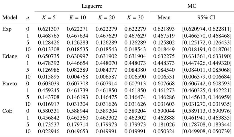
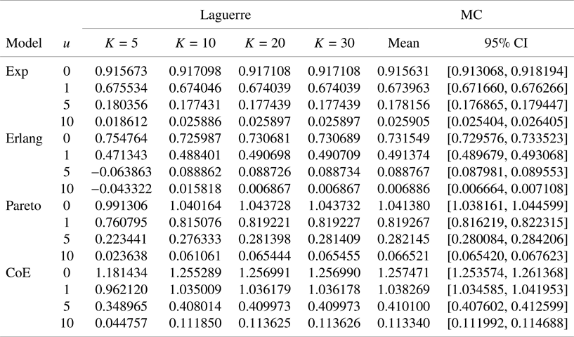
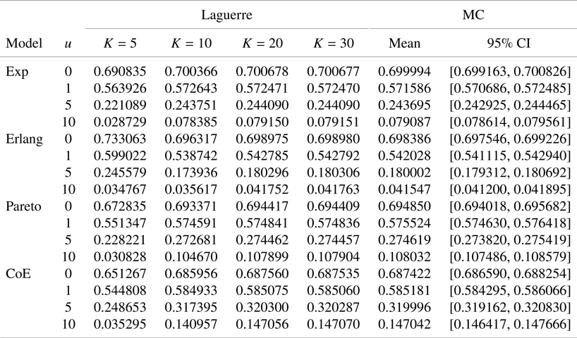
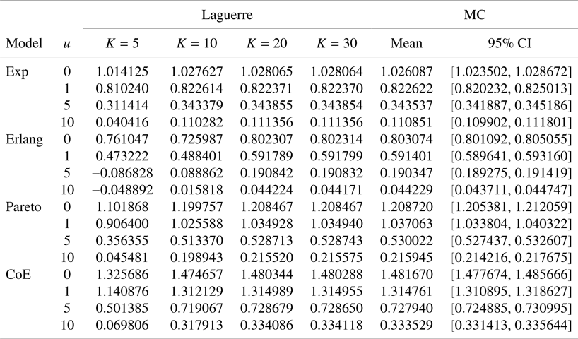
First, we test the accuracy of the Laguerre series expansion method. It is known that there are no explicit formulas for the Gerber-Shiu functions under fixed periodic observation. Hence, in order to provide benchmark results, we perform Monte Carlo simulation for each risk model. Both the mean values and the 95% confidence intervals will be calculated based on $10^{6}$ sample paths of the surplus processes. In Tables 1–4, we report the numerical results for the finite-time Gerber-Shiu function $\phi (u;T)$ with $\delta =0.01$, $\Delta =1$ and (i) $T=10$, $w\equiv 1$; (ii) $T=10$, $w(x)=x$; (iii) $T=50$, $w\equiv 1$ and (iv) $T=50$, $w(x)=x$. For these two penalty functions, the finite-time Gerber-Shiu functions are respectively the Laplace transform of the ruin time and the expected discounted value of the deficit at ruin when ruin occurs within the first $T/\Delta$ observation times.

Table 1.

Approximating results of $\phi (u,T)$, $T=10$, $w\equiv 1$.

Table 2.

Approximating results of $\phi (u,T)$, $T=10$, $w(x)=x$.

Table 3.

Approximating results of $\phi (u,T)$, $T=50$, $w\equiv 1$.

Table 4.

Approximating results of $\phi (u,T)$, $T=50$, $w(x)=x$.

In each table, we set the initial surplus level $u=0$, 1, 5, 10, and take the truncation parameter $K=5$, 10, 20, 30. It follows from each row (i.e., $u$ is fixed) that the approximation performance gets better as $K$ becomes larger, and the values are stable when $K$ is $30$. Compared with the Monte Carlo values, we can find that each relative error of Laguerre series expansion is controlled within $1\%$, and the approximate values are well covered by each of the confidence intervals. On the other hand, fix the truncation parameter $K$, we observe from each column that the finite-time Gerber-Shiu function is a decreasing function of the initial surplus level $u$.

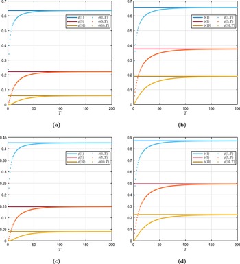
Next, we study the impact of the observation parameters $T$ and $\Delta$ on the finite-time Gerber-Shiu functions. Set $\delta =0.01$. Fix the initial surplus level $u=1$, 5, 10 and the inter-observation time $\Delta =0.01$. In Figure 1, we plot the curves for the finite-time Gerber-Shiu functions for different claim size density functions and penalty functions. Note that $\phi (u;T)=\phi _n(u)$ with $n=T/\Delta$. The curves are plotted based on the Laguerre series expansion $\hat {\phi }_n(u)$ with truncation parameter $K=30$. As expected, each finite-time Gerber-Shiu function is an increasing function of $T$. This fact is very intuitive, since the larger the observation interval $[0, T]$, the more likely we can monitor the ruin event. It is easily seen from Figure 1 that $\phi (u;T)\rightarrow \phi (u)$. In fact, we can find that $\phi (u,T)\approx \phi (u)$ when $T\geq 150$. The limit is obvious due to the monotone convergence theorem. On the other hand, we note that the difference between $\phi (u)$ and $\phi (u;T)$ is the following $T$-deferred Gerber-Shiu function

(7.1)\begin{equation} \bar{\phi}(u;T)=E[e^{-\delta \tau} w(|U_{\tau}|) \mathbf{1}_{\{T<\tau<\infty\}} |U_0=u],\quad u\geq 0. \end{equation}

Under the additional condition $E[e^{-\delta \tau } \tau ^{k} w(|U_{\tau }|) \mathbf {1}_{\{\tau <\infty \}} |U_0=u]<\infty$ for $k>0$, Markov's inequality yields

$$\bar{\phi}(u;T)\leq \frac{1}{T^{k}}E[e^{-\delta \tau} \tau^{k} w(|U_{\tau}|) \mathbf{1}_{\{\tau<\infty\}} |U_0=u].$$

Hence, we have $\phi (u;T)-\phi (u)=O(T^{-k})$.

FIGURE 1.

Convergence of $\phi (u;T)$ for increasing $T$. $\Delta =0.01$, $u=1, 5, 10$. (a) Erlang, $w\equiv 1$; (b) CoE, $w\equiv 1$; (c) Erlang, $w(x)=x$; (d) Pareto, $w(x)=x$.

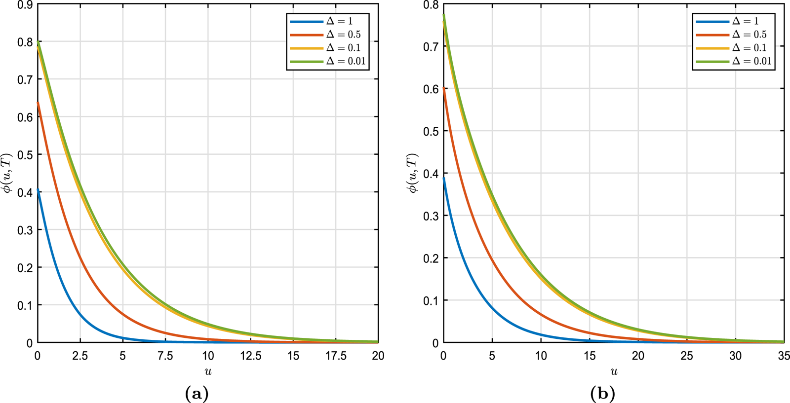
In Figure 2, we plot the finite-time Gerber-Shiu functions (with $\delta =0.01$ and $w\equiv 1$) on fixed observation interval $[0, 50]$, but with different observation frequency, $\Delta =1$, 0.5, 0.1, 0.01. Again, we find that under each observation frequency, the finite-time Gerber-Shiu functions are decreasing w.r.t. the initial surplus level $u$. By Figure 2, we can also find that the corresponding finite-time Gerber-Shiu functions increase as $\Delta$ decreases, which may be due to that ruin is more likely to be monitored as the observation frequency increases. On the other hand, when fixing the initial surplus level $u$, we can observe from Figure 2 the convergence behavior of the finite-time Gerber-Shiu functions w.r.t. $\Delta$. 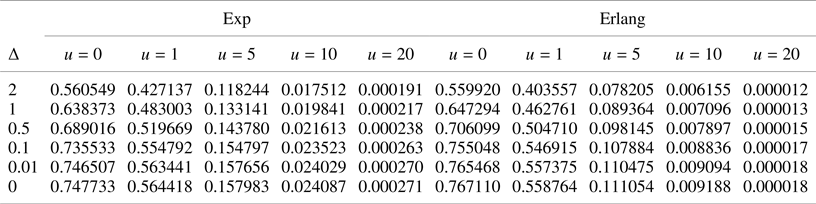In fact, as $\Delta \rightarrow 0$, the finite-time Gerber-Shiu functions will converge to those under continuous observation. 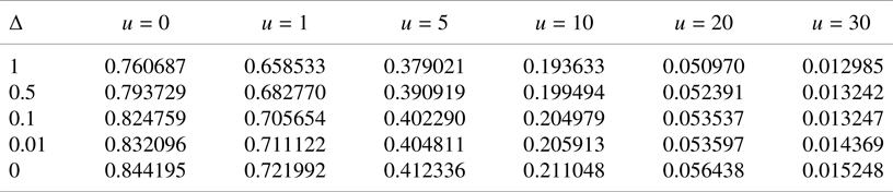To test this convergence behavior, we set $T=10$ and compute the finite-time ruin probabilities with $\Delta =2$, 1, 0.5, 0.1, 0.01, 0. Note that the case $\Delta =0$ corresponds to continuous observation. In Table 5, we list the numerical results for exponential and Erlang(2,2) claim size density functions, where the results in the last row could be computed by formulas in Garcia [Reference Garcia15] and Dickson [Reference Dickson11]. It follows from each column that the finite-time ruin probabilities under periodic observation converge to the values under continuous observation.

FIGURE 2.

Finite-time Gerber-Shiu functions vs. initial surplus $u$. $T=50$, $\Delta =1, 0.5, 0.1, 0.01$. (a) Erlang; (b) CoE.

Table 5.

Approximating results of finite-time ruin probability under different $\Delta$.

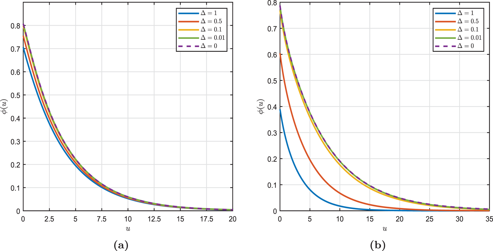
Finally, we study the infinite-time Gerber-Shiu functions under periodic observation. Set $\delta =0.01$, $w\equiv 1$, and consider the Erlang(2,2) and CoE claim size density functions. In Figure 3, we plot the infinite-time Gerber-Shiu functions for different claim size density functions. For periodic observation, we set $\Delta =1, 0.5, 0.1, 0.01$, and plot the curves for the infinite-time Gerber-Shiu functions based on formula (6.11) with truncation parameter $K=30$. We also consider the case $\Delta =0$ (i.e., continuous observation), and plot the curves for the infinite-time Gerber-Shiu functions based on the following formulas,

• • Erlang: $\phi (u)=0.8287e^{-0.2626u}-0.0216e^{-2.9390u},\ u\geq 0;$

• • CoE: $\phi (u)=0.7431e^{-0.1360u}+0.0444e^{-1.5615u},\ u\geq 0$.

The above formulas can be easily obtained by a Laplace transform inversion method. It follows from Figure 3 that all the infinite-time Gerber-Shiu functions are decreasing functions of the initial surplus level $u$. While for each fixed initial surplus level, $\phi (u)$ increase as $\Delta$ decreases, and furthermore, they all converge to those under continuous observation.

FIGURE 3.

Infinite-time Gerber-Shiu functions vs. initial surplus $u$. $\Delta =1, 0.5, 0.1, 0.01$. (a) Erlang; (b) CoE.

In Table 6, we report some approximation results for the infinite-time ruin probability with Pareto claim size density function. Set $\delta =0$, $w\equiv 1$, $\Delta =1$, 0.5, 0.1, 0.01, and compute the ruin probabilities based on formula (6.11) with truncation parameter $K=30$. We also list some numerical results for ruin probability with continuous observation, where the results are computed by formula (20) in Ramsay [Reference Ramsay25]. From each column in Table 6, we find that the ruin probabilities increase as $\Delta$ decreases, and they converge to the corresponding values under continuous observation.

Table 6.

Approximating results of infinite-time ruin probability with Pareto distribution.