Dynamics of a magnetic particle in an oscillating magnetic field subject to a shear flow

I. Misra; V. Kumaran

doi:10.1017/jfm.2024.436

Dynamics of a magnetic particle in an oscillating magnetic field subject to a shear flow

Published online by Cambridge University Press: 25 July 2024

I. Misra

and

V. Kumaran

Show author details

I. Misra: Affiliation:
Department of Chemical Engineering, Indian Institute of Science, Bangalore 560 012, India
V. Kumaran*: Affiliation:
Department of Chemical Engineering, Indian Institute of Science, Bangalore 560 012, India
*: †Email address for correspondence: kumaran@iisc.ac.in

Article contents

Abstract
Introduction
Evolution equations
Limiting cases
Asymptotic solutions
Results
Conclusions
Funding
Declaration of interests
References

Rights & Permissions

Abstract

The orientational dynamics of a spherical magnetic particle in linear shear flow subjected to an oscillating magnetic field in the flow plane is analysed in the viscous limit. The shear is in the $X$–$Y$ plane, the magnetic field is in the $X$ direction and the vorticity is perpendicular to the flow in the $Z$ direction. The relevant dimensionless groups are $\omega ^\ast$, the ratio of the frequency of the magnetic field and the strain rate, and $\varSigma$, the ratio of the magnetic and hydrodynamic torques. As $\varSigma$ is decreased, there is a transition from in-plane rotation, where the rotation is in the flow ($X$–$Y$) plane, to out-of-plane rotation, where the orientation vector is not necessarily in the $X$–$Y$ plane and the dynamics depends on the initial orientation. The particle rotation is phase-locked for in-plane rotation with discrete odd rotation number (number of rotations in one period of magnetic field oscillation), while the orbits are quasi-periodic with non-integer rotation number for out-of-plane rotation. For $\varSigma \gg 1$, regions of odd rotation number $n_o$ are bound by the lines $8 (n_o-1) \varSigma \omega ^\ast = 1$ and $8 (n_o+1) \varSigma \omega ^\ast = 1$, and there are discontinuous changes in the rotation number and mean and root-mean-square torque at these lines. For $\varSigma \ll 1$, the domains of in-plane rotation of finite width in the $\omega ^\ast$–$\varSigma$ plane extend into downward cusps at $\omega ^\ast = {1}/{2 n_o}$. The orbits are quasi-periodic between these domains, where the rotation is out of plane.

JFM classification

Complex Fluids: Suspensions

Information

Type: JFM Papers
Information: Journal of Fluid Mechanics , Volume 988 , 10 June 2024, A49
DOI: https://doi.org/10.1017/jfm.2024.436 [Opens in a new window]
Creative Commons: This is an Open Access article, distributed under the terms of the Creative Commons Attribution licence (http://creativecommons.org/licenses/by/4.0), which permits unrestricted re-use, distribution and reproduction, provided the original article is properly cited.
Copyright: © The Author(s), 2024. Published by Cambridge University Press.

1. Introduction

Magnetorheological fluids are suspensions of magnetic particles in a viscous fluid. The particles are usually of micrometre size, are multi-domain and could have permanent or induced dipoles. The particles are randomly oriented in the absence of a magnetic field, and they flow like a homogeneous fluid. When a field is applied, the particles align along the field direction. Due to particle interactions, the particles also cluster into rigid elongated structures along the field direction. The transition between the homogeneous and clustered states takes place in a few milliseconds. This clustering could be used to control the flow in conduits, from a freely flowing state in the absence of a field to a jammed state when a field is applied. Due to this, magnetorheological fluids are used in applications requiring rapid response, such as brakes and dampers (Klingenberg Reference Klingenberg2001; de Vicente, Klingenberg & Hidalgo-Alvarez Reference de Vicente, Klingenberg and Hidalgo-Alvarez2011). The torques acting on a particle are of two types – a hydrodynamic torque due to shear and a magnetic torque due to the magnetic field. The ratio of these is the dimensionless Mason number (Sherman, Becnel & Wereley Reference Sherman, Becnel and Wereley2015). In the presence of a magnetic field, the rheology of the fluid is characterised by a ‘yield stress’, which is the minimum stress required to disrupt the clustered particles and generate flow (Kuzhir, Lopez-Lopez & Bossis Reference Kuzhir, Lopez-Lopez and Bossis2009; Lopez-Lopez, Kuzhir & Bossis Reference Lopez-Lopez, Kuzhir and Bossis2009; de Vicente et al. Reference de Vicente, Segovia-Gutierrez, Andablo-Reyes, Vereda and Hidalgo-Alvarez2009; Anupama, Kumaran & Sahoo Reference Anupama, Kumaran and Sahoo2018). The Bingham number is the ratio of the yield stress and the shear stress applied on the fluid (Barnes, Hutton & Walters Reference Barnes, Hutton and Walters1989). The rheology has been characterised by a relation between the Mason and Bingham numbers (Sherman et al. Reference Sherman, Becnel and Wereley2015). The yield stress has been derived using particle-based models (Klingenberg & Zukoski Reference Klingenberg and Zukoski1990; Vagberg & Tighe Reference Vagberg and Tighe2017).

An alternative interpretation of the jamming of magnetorheological fluids is the instability and spontaneous growth of concentration fluctuations due to interparticle hydrodynamic and magnetic interactions (Kumaran Reference Kumaran2022). It has been shown that the effect of interactions can be expressed as an anisotropic diffusion matrix for the concentration field, in which concentration fluctuations are damped in the direction of the magnetic field and amplified in the directions perpendicular to the magnetic field. This could result in the formation of anisotropic clusters along the field direction. One area that has not been explored is the effect of oscillating magnetic fields on the jamming in magnetorheological fluids. As a first step in this direction, we examine the dynamics of one magnetic particle in an oscillating magnetic field subject to a shear flow.

Ferrofluids are nanometre-sized particles, usually single domain, with a permanent magnetic moment suspended in a fluid. These are well dispersed with random orientation due to thermal fluctuations in the absence of a magnetic field. The particles align and form interesting shapes in the presence of a magnetic field. The ‘spin-up’ flow of ferrofluids in the presence of a magnetic field has been an area of active study (Moskowitz & Rosensweig Reference Moskowitz and Rosensweig1967; Zaitsev & Shliomis Reference Zaitsev and Shliomis1969; Chaves, Zahn & Rinaldi Reference Chaves, Zahn and Rinaldi2008). A salient characteristic of the flow of ferrofluids is the presence of an antisymmetric component in the stress tensor proportional to the difference in the particle angular velocity and the fluid rotation rate, this difference caused by the magnetic torque on the particles. In addition to the mass and linear momentum equations, an angular momentum equation is formulated, which contains a term similar to the divergence of the stress due to the gradients in the particle angular velocity (Rosensweig Reference Rosensweig2000; Rinaldi & Zahn Reference Rinaldi and Zahn2002). Here, we characterise the torque on a magnetic particle due to an applied magnetic field. This can be used to derive a constitutive relation for a suspension of magnetic particles subject to an oscillating field, because the torque is directly related to the antisymmetric part of the stress tensor in the viscous limit (Batchelor Reference Batchelor1970).

Magnetic particles have been used for mixing different fluids in microfluidic applications. The flow Reynolds number is usually low in microfluidic applications, and the flow is in the laminar regime. Cross-stream molecular diffusion does not generate sufficiently fast mixing for practical applications (Abbasi et al. Reference Abbasi, Chowdhury, Subramaniam, Jain, Muthe, Sheikh, Banerjee and Kumaran2019), and different passive strategies (Ward & Fan Reference Ward and Fan2015) and active strategies have been proposed for enhancing mixing. One of these is to use time-varying magnetic fields to enhance mixing (Shanko et al. Reference Shanko, van de Burgt, den Anderson and Toonder2019). Different strategies have been used, such as magnetically actuated cilia (Khaderi et al. Reference Khaderi, Baltussen, Anderson, den Toonder and Onck2010; Wu et al. Reference Wu, Panigrahi, Lu and Chen2017) and magnetic beads (Kang et al. Reference Kang, Hulsen, Anderson, den Toonder and Meijer2007; Gao et al. Reference Gao, van Reenen, Hulsen, de Jong, Prins and den Toonder2014). The moving elements such as cilia or beads are actuated by rotating or chaotic magnetic fields. Despite the studies in this important application, there are currently no models that can predict mixing efficiency based on the parameters characterising the particle and the magnetic field. Here, we study the dynamics of an isolated particle subject to an oscillating magnetic field. The time variation of the particle orientation, the mean torque exerted on the fluid and the root mean square of the torque fluctuations are calculated as a function of the magnetic field, frequency and the fluid and particle properties. The mean torque can be used to generate secondary flows due to the antisymmetric part of the rate of deformation tensor, and the fluctuating torque generates velocity fluctuations which can be calculated from the Stokes equation. This is the first step in characterising mixing due to magnetic particles in a time-varying magnetic field.

There have been relatively few studies on the dynamics of a spheroidal magnetic particle subjected to a shear flow and a magnetic field (Almog & Frankel Reference Almog and Frankel1995; Sobecki et al. Reference Sobecki, Zhang, Zhang and Wang2018; Kumaran Reference Kumaran2020a). The particle was considered to have a permanent dipole with constant magnetic moment aligned along the axis of the spheroid. The orientation dynamics depends on the dimensionless ratio of the magnetic and hydrodynamic torques, denoted by the dimensionless parameter $\varSigma$. In the absence of a magnetic field, a spheroid in a linear shear flow in the viscous limit undergoes closed ‘Jeffery orbits’ (Jeffery Reference Jeffery1923; Hinch & Leal Reference Hinch and Leal1979). The effect of thermal noise on the orientation distribution has been studied (Kumar & Ramamohan Reference Kumar and Ramamohan1995; Asokan, Ramamohan & Kumaran Reference Asokan, Ramamohan and Kumaran2002). In the limit of zero shear, the particle aligns along the direction of the magnetic field. As $\varSigma$ is increased, one would expect the particle to undergo a transition from a rotating to a static state. However, the phase portraits for spheroids are complex with multiple stationary points and limit cycles. Depending on the aspect ratio and the ratio of the magnetic and hydrodynamic torques, the phase portrait could contain two to six stationary nodes and/or a limit cycle. The complex phase portraits result from a relatively simple series of bifurcations in the three-dimensional parameter space consisting of $\varSigma$ and the two orientation angles. Depending on the aspect ratio of the spheroid, there could be up to two saddle-node bifurcations, two subcritical bifurcations and one reverse saddle-node bifurcation due to the merger of stationary points.

The studies of Almog & Frankel (Reference Almog and Frankel1995), Sobecki et al. (Reference Sobecki, Zhang, Zhang and Wang2018) and Kumaran (Reference Kumaran2020a) for particles with a permanent dipole were extended to spheroidal particles with an induced dipole in Kumaran (Reference Kumaran2021a,Reference Kumaranb). Here, different magnetisation models were considered for the particle magnetic moment. The magnetic moment is a linear function of the component of the magnetic field along the axis in the linear model, while it is a step function in the signum model. The Langevin model was also considered where there is a transition between a constant magnetic moment for high magnetic field and a linear function of the magnetic field component along the particle axis for low magnetic field. When the magnetic field is in the flow plane, an analytical solution was obtained for the linear model for the transition between stationary and rotating states. A complex phase portrait was observed for the signum model, including transitions between static and rotating states that could be continuous or discontinuous and the existence of multiple steady states. When the magnetic field is not in the flow plane, the particle aligns along the field direction for high magnetic field. There could be one steady state with orientation almost perpendicular to the flow plane and one rotating state with orientation close to the flow plane. Thus, complex dynamical behaviour is observed in a relatively simple configuration of a magnetic particle in a steady magnetic field subjected to a shear flow.

There have been some studies on the effect of a magnetic field on conducting particles subject to a shear flow (Moffat Reference Moffat1990; Kumaran Reference Kumaran2019, Reference Kumaran2020b). A conducting particle in a shear flow rotates in the viscous limit with angular velocity equal to one half of the vorticity. Eddy currents are induced in a particle rotating in a magnetic field due to Faraday's law. The eddy currents result in a magnetic moment on the particle in accordance with Ampere's law. The interaction between the magnetic moment and the field causes a torque which tends to decrease the angular velocity of the particle. The trajectories of the particle in a time-varying magnetic field have been calculated (Moffat Reference Moffat1990), and the antisymmetric part of the stress tensor due to the torque on the particle in a constant magnetic field has been derived in the dilute limit in the absence of particle interactions (Kumaran Reference Kumaran2019, Reference Kumaran2020b).

The motion of a dipolar spherical particle in a time-periodic magnetic field was studied by Puyesky & Frankel (Reference Puyesky and Frankel1998), who found that the motion could be of two types: phase-locked periodic motion and quasi-periodic motion. The authors obtained a condition for the existence of phase-locked periodic motion when the magnetic field is in the direction of shear. The parameter regimes for phase-locked and quasi-periodic motion were identified for a piecewise constant periodic function which transitions periodically and discontinuously between ${\pm }1$. The orbits were periodic with integer rotation number for the phase-locked motion when the magnetic torque is much larger than the hydrodynamic torque, and quasi-periodic with a continuous variation in rotation number when the magnetic torque is small compared with the hydrodynamic torque. However, even in the limit of small magnetic torque, there were regions of parameter space where there is phase-locked motion having the structure of Arnold tongues.

The ‘circle maps’ in dynamical systems provide a context for understanding some of the unusual features of the present system. The equation for the angle $\phi$ of a single forced oscillator such as a Josephson junction or a charge density wave (Jensen, Bak & Bohr Reference Jensen, Bak and Bohr1983; Bak et al. Reference Bak, Bohr, Hogh Jensen and Voetmann Christiansen1984; Bohr, Bak & Jensen Reference Bohr, Bak and Jensen1984; Rosenblum & Pikovsky Reference Rosenblum and Pikovsky2003) is of the form

(1.1)

\begin{equation} \frac{\mbox{d} \phi}{\mbox{d} t} + \sin{(\phi)} = A + B \sin{(\omega t)}, \end{equation}

where $A$ is the constant frequency and $B$ is the coupling constant multiplying the forcing function. A second derivative of $\phi$ with respect to time is also usually present in (1.1), which is neglected here for simplicity. Equation (1.1) can be transformed into a map because it is invariant under the transformation $\phi \rightarrow \phi + 2 {\rm \pi}$. In this case, (1.1) can be transformed into a mapping relating the value of $\phi$ at time instant $t$ and a later time instant $t+(2 {\rm \pi}/\omega )$, since the equality is satisfied at both these time instants:

(1.2)

\begin{equation} \phi(t+2{\rm \pi}/\omega) = g(\phi(t)). \end{equation}

The standard circle map has the form

(1.3)

\begin{equation} \phi(t+2{\rm \pi}/\omega) = \phi(t) + \varOmega - \frac{K \sin{(2 {\rm \pi}\phi)}}{2 {\rm \pi}}, \end{equation}

where $\varOmega$ is the angular velocity and $K$ is the coupling constant for the map. The circle map has the following characteristics.

(i) For $K = 0$, the evolution of $\phi$ is periodic with rotation number $N$ if $\varOmega$ is the ratio of prime numbers $M/N$, and is quasi-periodic otherwise. For $0 < K \ll 1$, the periodic or phase-locked oscillations occur over a finite range of $\varOmega$. The plot of the rotation number versus $\varOmega$ has a step-like appearance, and is referred to as the Devil's staircase (Jensen et al. Reference Jensen, Bak and Bohr1983). The regions of phase-locked rotation in the $\varOmega$–$K$ plane have cusps in the limit $K \ll 1$ and branch out into finite ‘Arnold tongues’ (Arnold Reference Arnold1961; Glass & Perez Reference Glass and Perez1982) as $K$ is increased. The rotation is quasi-periodic between the Arnold tongues.
(ii) The map has a critical point at $K=1$, with a cubic singularity of the inverse mapping at $\phi = 0$. The Arnold tongues merge, and the system transitions between different winding numbers.
(iii) There could be chaos for $K>1$, because the map (1.3) is not invertible.

The dynamics of the meridional angle $\phi$ of the particle orientation is compared with those for circle maps in § 6.

The dynamics of a spherical magnetic field subject to a shear flow and a sinusoidal oscillating magnetic field is analysed here. Following the analysis of Puyesky & Frankel (Reference Puyesky and Frankel1998) for a piecewise constant field, we consider the more realistic case of a sinusoidal field for which analytical results cannot be easily derived. Analytical results for the phase boundaries cannot be derived for a general sinusoidal modulation, and so we carry out a numerical analysis of the dynamics in different parameter regimes. Regions of phase-locked and quasi-periodic orbit are identified in a phase diagram consisting of two parameters: the ratio of the magnetic and hydrodynamic torques $\varSigma$ and the ratio of the frequency of oscillations and the applied strain rate $\omega ^\ast$. This parameter space enables the validation of the results against the limiting cases, that is, $\varSigma \gg 1$ where the magnetic torque is much larger than the hydrodynamic torque, $\varSigma \ll 1$ where the hydrodynamic torque is much larger than the magnetic torque and $\omega ^\ast \ll 1$ which is a steady magnetic field. Puyesky & Frankel (Reference Puyesky and Frankel1998) found that the limit $\varSigma \ll 1$ is singular due to the presence of Arnold tongues. Here, we find that the other two limits are also singular in different ways.

An important objective of the present analysis is to calculate the torque exerted by the particle on the fluid, since this is the cause of secondary flows and mixing. The mean and the root mean square of the torques on the fluid are calculated using asymptotic analysis in the limits of low and high $\varSigma$, and these are compared with the numerical results. An important finding is the discontinuous transition between phase-locked orbits of different rotation number which result in discontinuous changes in the torque on the fluid.

2. Evolution equations

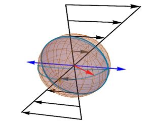
The configuration and coordinate system are shown in figure 1. A spherical particle with diameter $d$ and permanent magnetic moment $\boldsymbol {m} = m \boldsymbol {o}$ is subjected to a shear flow in the $x$–$y$ plane, and an oscillating magnetic field. Here, the orientation vector $\boldsymbol {o}$ is the unit vector along the direction of the magnetic moment and $\boldsymbol {e}_X$ is the unit vector in the $X$ direction. The azimuthal angle $\theta$ is the angle between the orientation vector and the $Z$ axis, and the meridional angle $\phi$ is the angle made by the projection of the orientation vector on the $X$–$Y$ plane with the $X$ axis. The flow velocity is

(2.1)

\begin{equation} \boldsymbol{v} = \dot{\gamma} Y \boldsymbol{e}_X, \end{equation}

where $\dot {\gamma }$ is the strain rate. The vorticity is

(2.2)

\begin{equation} \mbox{Vorticity} = \boldsymbol{\nabla} \times \boldsymbol{v} ={-} \dot{\gamma} \boldsymbol{e}_Z, \end{equation}

where $\boldsymbol {e}_Z$ is the unit vector along the $Z$ axis. The magnetic field varies sinusoidally in time with frequency $\omega$:

(2.3)

\begin{equation} \boldsymbol{H} = H_0 \cos{(\omega t)} \boldsymbol{e}_X. \end{equation}

The rate of change of the orientation vector is equal to the tangential velocity of the particle:

(2.4)

\begin{equation} \frac{\mbox{d} \boldsymbol{o}}{\mbox{d} t} = \boldsymbol{\varOmega} \boldsymbol{\times} \boldsymbol{o}, \end{equation}

where $\boldsymbol {\varOmega }$ is the angular velocity of the particle. The angular velocity is determined from the torque balance which reduces to the following in the viscous limit where inertial forces are neglected:

(2.5)

\begin{equation} {\rm \pi}\mu d^3 \left(-\tfrac{1}{2} \dot{\gamma} \boldsymbol{e}_Z - \boldsymbol{\varOmega}\right) + \boldsymbol{m} \boldsymbol{\times} \boldsymbol{H} = 0. \end{equation}

The first term on the left-hand side in (2.5) is the hydrodynamic torque on the particle due to the difference between the fluid rotation rate which is one-half of the vorticity, $- \frac {1}{2} \dot {\gamma } \boldsymbol {e}_Z$, and the particle rotation rate, $\boldsymbol {\varOmega }$. The second term on the left-hand side in (2.5) is the magnetic torque $\boldsymbol {m} \boldsymbol {\times } \boldsymbol {H}$ on the particle.

Figure 1.

Configuration and coordinate system for analysing the dynamics of a spherical particle with a magnetic dipole (red arrow) in an oscillating magnetic field along the $X$ direction (blue arrow) and subjected to a shear flow in the $X$–$Y$ plane.

Equation (2.5) is substituted into (2.4) to obtain an equation for the rate of change of the orientation vector:

(2.6)

\begin{equation} \frac{\mbox{d} \boldsymbol{o}}{\mbox{d} t} ={-} \frac{1}{2} \dot{\gamma} \boldsymbol{e}_Z \boldsymbol{\times} \boldsymbol{o} + (m /{\rm \pi} d^3 \mu) (\boldsymbol{H} - \boldsymbol{o} (\boldsymbol{o} \boldsymbol{\cdot} \boldsymbol{H})). \end{equation}

Here, the magnetic moment is expressed as $\boldsymbol {m} = m \boldsymbol {o}$, and the identity $(\boldsymbol {a} \boldsymbol {\times } \boldsymbol {b}) \boldsymbol {\times } \boldsymbol {c} = \boldsymbol {b} (\boldsymbol {a} \boldsymbol {\cdot } \boldsymbol {c}) - \boldsymbol {a} (\boldsymbol {b} \boldsymbol{\cdot} \boldsymbol {c})$ has been used to simplify equation (2.6). The expression (2.3) for the magnetic field is substituted into (2.6), and the scaled time is defined as $t^\ast = \dot {\gamma } t$, to obtain the dimensionless equation

(2.7)

\begin{equation} \frac{\mbox{d} \boldsymbol{o}}{\mbox{d} t^\ast} ={-} \frac{1}{2} \boldsymbol{e}_Z \boldsymbol{\times} \boldsymbol{o} + \varSigma \cos{(\omega^\ast t^\ast)} (\boldsymbol{e}_X - \boldsymbol{o} (\boldsymbol{o} \boldsymbol{\cdot} \boldsymbol{e}_X)), \end{equation}

where the dimensionless parameters $\varSigma$ and $\omega ^\ast$ are

(2.8)

\begin{gather} \varSigma = \frac{m H_0}{{\rm \pi} d^3 \mu \dot{\gamma}}, \end{gather}

(2.9)

\begin{gather}\omega^\ast= \frac{\omega}{\dot{\gamma}}. \end{gather}

The parameter $\varSigma$ is the ratio of the magnetic and hydrodynamic torques on the particle and the parameter $\omega ^\ast$ is the ratio of the magnetic field frequency and the applied strain rate.

Equation (2.7) is expressed in terms of the azimuthal and meridional angles, $\theta$ and $\phi$:

(2.10)

\begin{gather} \frac{\mbox{d} \theta}{\mbox{d} t^{{\ast}}} = \varSigma \cos{(\omega^\ast t^\ast)} \cos{(\theta)} \cos{(\phi)}, \end{gather}

(2.11)

\begin{gather}\frac{\mbox{d} \phi}{\mbox{d} t^{{\ast}}} ={-} \frac{1}{2} - \varSigma \cos{(\omega^\ast t^\ast)} \csc{(\theta)} \sin{(\phi)}. \end{gather}

These equations are solved to obtain the time variation of $\theta$ and $\phi$. For $\varSigma \gg 1$, where the magnetic torque is much larger than the hydrodynamic torque, it is appropriate to define the scaled time as $t^{{{\dagger}}} = (t m H_0/{\rm \pi} \mu d^3)$, and the evolution equations are

(2.12)

\begin{gather} \frac{\mbox{d} \theta}{\mbox{d} t^{{{{\dagger}}}}} = \cos{(\omega^{{{\dagger}}} t^{{{\dagger}}})} \cos{(\theta)} \cos{(\phi)}, \end{gather}

(2.13)

\begin{gather}\frac{\mbox{d} \phi}{\mbox{d} t^{{{{\dagger}}}}} ={-} \frac{1}{2} \varSigma^{{-}1} - \cos{(\omega^{{{\dagger}}} t^{{{\dagger}}})} \csc{(\theta)} \sin{(\phi)}, \end{gather}

where $\omega ^{{{\dagger}}} = {\rm \pi}\mu d^3 \omega /m H_0$.

The torque in the $X$ direction, which is the direction of the magnetic field, is zero, because the torque is the cross product of the magnetic field and the particle moment. The torques in the $Y$ and $Z$ directions are scaled by the characteristic viscous torque ${\rm \pi} \mu d^3 \dot {\gamma }$:

(2.14)

\begin{equation} \left.\begin{gathered} T_Y^\ast= T_Y/({\rm \pi} \mu d^3 \dot{\gamma}) = \varSigma \cos{(\theta)} \cos{(\omega^\ast t^\ast)}, \\ T_Z^\ast= T_Z/({\rm \pi} \mu d^3 \dot{\gamma}) ={-} \varSigma \sin{(\theta)} \sin{(\phi)} \cos{(\omega^\ast t^\ast)}. \end{gathered}\right\} \end{equation}

The average and the root mean square of quantities such as the torque and angular velocity are defined as

(2.15)

\begin{equation} \left.\begin{gathered} \bar{\star} = \frac{1}{T_{av}} \int_0^{T_{av}} \mbox{d} t \star, \\ \overline{\bar{\star}} = \left(\frac{1}{T_{av}} \int_0^{T_{av}} \mbox{d} t ({\star} - \bar{\star})^2 \right)^{1/2}, \end{gathered}\right\} \end{equation}

where the averaging time $T_{av}$ is much larger than the time periods of the Jeffery orbit and the magnetic field oscillation.

For the special case of in-plane rotation $\theta = ({\rm \pi} /2)$, where the particle orientation is in the plane of shear, (2.10) is identically satisfied. Equation (2.11) for $\phi$ can be expressed in terms of the torque:

(2.16)

\begin{equation} \frac{\mbox{d} \phi}{\mbox{d} t^{{\ast}}} ={-} \frac{1}{2} + T_Z^\ast. \end{equation}

The average torque can be calculated using the definition (2.15):

(2.17)

\begin{align} \bar{T}_Z^\ast &= \frac{1}{T_{av}} \left( \int_0^{T_{av}} \mbox{d} t^\ast \frac{\mbox{d} \phi}{\mbox{d} t^{{\ast}}} \right) + \frac{1}{2} \nonumber\\ &= \bar{\varOmega}^\ast_Z + \frac{1}{2} = R^\ast \omega^\ast + \frac{1}{2}. \end{align}

Here, $\varOmega _Z^\ast = (\mbox {d} \phi /\mbox {d} t^\ast )$ is the scaled instantaneous angular velocity of the particle about the $Z$ axis, $\bar {\varOmega }^\ast _Z$ is the average angular velocity defined by (2.15) and

(2.18)

\begin{equation} R^\ast= (\bar{\varOmega}^\ast_Z/\omega^\ast) \end{equation}

is the rotation number, which is the number of rotations of the particle within one time period of the magnetic field oscillation. It should be noted that $\varOmega _Z^\ast$ is negative when the particle rotates in the clockwise direction.

There are three time scales: the inverse of the strain rate $\dot {\gamma }^{-1}$, the inverse of the frequency $\omega ^{-1}$ and a time scale $({\rm \pi} \mu d^3/m H_0)$ which is the characteristic relaxation time for the particle orientation when subjected to a magnetic field in the absence of shear. The two dimensionless groups $\varSigma$ and $\omega ^\ast$ (2.8)–(2.9) can be interpreted as ratios of these two time scales. The parameter $\varSigma = (m H_0 / {\rm \pi}\mu d^3 \dot {\gamma })$ is the ratio of the inverse of the strain rate and the magnetic response time. The parameter $\omega ^\ast$ is the ratio of the magnetic frequency and the strain rate and $\omega ^{{{\dagger}}} = (\omega {\rm \pi}\mu d^3/m H_0)$ is the product of the frequency and the relaxation time of the particle under an imposed magnetic field.

In the present analysis, attention is restricted to the long-time limit when the orbits have attained a periodic or quasi-periodic state. For in-plane rotation, the trajectory in the long-time limit is independent of the initial condition, though there are transients at short time which do depend on the initial condition. For out-of-plane rotation, the trajectory does depend on initial condition in the long-time limit. All figures for the time variation of the angles $\theta$ and $\phi$ are shown only for the long-time limit. It is important to note that $t^\ast = 0$ in these figures corresponds to the start of one oscillation in the magnetic field amplitude in the limit of long time.

3. Limiting cases

3.1. No magnetic field

For the Jeffery orbits in the absence of a magnetic field for a spherical particle, the azimuthal angle $\theta$ is a constant from (2.10), and the meridional angle $\phi = \phi _i - \frac {1}{2} t^\ast$ from (2.11), where $\phi _i$ is the angle at $t^\ast =0$. Thus, the particle rotates with a constant angular velocity about the axis perpendicular to the flow plane. The angular velocity is a constant, $\varOmega _Z^\ast = - \frac {1}{2}$, the rotation number is $R^\ast = - (1/2 \omega ^\ast )$ and the torque is zero.

3.2. No oscillation

The dynamics of a spheroid in a steady magnetic field subjected to a shear flow has been analysed in Kumaran (Reference Kumaran2020a). In the limit of high magnetic field, the orientation of the magnetic moment is steady, and it is aligned close to the direction of the applied magnetic field. In the limit of low magnetic field there is a rotating state similar to the Jeffery orbit but modified due to the magnetic field. There is a transition between rotating and steady states when the magnetic field is increased.

For a spherical particle with a permanent dipole, there is a transition between the steady and rotating states at $\varSigma = 0.5$. For $\varSigma > 0.5$, there are two fixed points, $(\theta _s, \phi _s)$, with particle moment aligned in the flow plane:

(3.1a,b)

\begin{equation} \theta_s = ({\rm \pi}/2),\quad \sin{(\phi_s)} ={-} \frac{1}{2 \varSigma}. \end{equation}

The fixed point for $0 < \phi _s < {\rm \pi}/2$ is a stable fixed point, while that for $-{\rm \pi} /2 < \phi _s < 0$ is an unstable fixed point. For $\varSigma < 0.5$, there are two neutral points located at

(3.2a,b)

\begin{equation} \sin{(\theta_s)}^2 = 4 \varSigma^2,\quad \phi_s ={-} ({\rm \pi}/2), \end{equation}

and there are periodic orbits around these two neutral points.

3.3. No shear

The dynamics in the absence of shear is discussed in Appendix A. Under an oscillatory magnetic field, the particle orientation vector oscillates on great circles on a unit sphere that intersect on the poles along the magnetic field direction. The dynamics depends on one dimensionless parameter, $\omega ^{{{\dagger}}} = (\omega {\rm \pi}d^3 \mu /m H) = (\omega ^\ast /\varSigma )$. For $\omega ^{{{\dagger}}} \gg 1$, the period of the magnetic field oscillation is small compared with the relaxation time. The direction of the field reverses before the orientation changes very much, and the amplitude of the oscillation decreases proportional to $(\omega ^{{{{\dagger}}} })^{-1}$. In the opposite limit $\omega ^{{{\dagger}}} \ll 1$, the period of the magnetic field oscillation is much larger than the particle relaxation time. The orientation oscillates between extrema close to $\phi = 0$ and ${\rm \pi}$, which are the two poles on the unit sphere with axis along the magnetic field direction. The extrema of $\sin {(\phi )}$ scale as $\exp {(-1/\omega ^{{{\dagger}}} )}$, indicating that the orientation vector approaches very close to, but does not reach, $\phi = 0, {\rm \pi}$. Thus, the oscillatory forcing causes an oscillation of the orientation vector, but no rotation.

Anticipating the analysis in §§ 5.1.2 and 5.2.2, it is noted here that the dynamics in the limit $\varSigma \gg 1$ is qualitatively different from that in the absence of shear. For $\varSigma \gg 1$, the particle orientation vector is in the flow ($X$–$Y$) plane. The particle undergoes one complete rotation in the clockwise direction over one period of the magnetic field oscillation – the particle rotation number is $R^\ast = -1$, and the average particle angular velocity is $\bar {\varOmega }^\ast _Z = - \omega ^\ast$.

4. Asymptotic solutions

The asymptotic solutions in the limit $\varSigma \ll 1$ are modifications of the Jeffery orbits due to the magnetic torque. These are derived using a regular perturbation expansion in § 4.1, and are compared with the numerical results in § 5.1. The regular perturbation expansion for $\varSigma \ll 1$ is not valid for $\omega ^\ast = \frac {1}{2}$, where the rotation rate (one-half of the vorticity) is equal to the magnetic field frequency, and there is resonance. This special case is considered in § 4.2. In the limit $\varSigma \gg 1$, where the magnetic torque is much larger than the hydrodynamic torque, the orientation vector rotates in the plane of the magnetic field. The orientation is close to the direction of the magnetic field for most of the oscillation period, and it undergoes rapid rotation when the direction of the magnetic field reverses.

4.1. Low magnetic field

When $\varSigma \ll 1$, a regular perturbation expansion is used in the small parameter $\varSigma$, $\theta = \theta _0 + \varSigma \theta _1 + \varSigma ^2 \theta _2 + \cdots$ and $\phi = \phi _0 + \varSigma \phi _1 + \varSigma ^2 \phi _2 + \cdots$. The leading-order solutions are Jeffery solutions, $\theta = \theta _0 = \theta _i$ and $\phi = - \frac {1}{2} t^\ast + \phi _i$, where $\theta _i$ and $\phi _i$ are the initial values of $\theta$ and $\phi$ at $t^\ast = 0$. The first and second corrections are determined using a regular perturbation expansion of (2.10) and (2.11):

(4.1)

\begin{gather} \frac{\mbox{d} \theta_1}{\mbox{d} t^\ast} = \cos{(\theta_0)} \cos{(\phi_0)} \cos{(\omega^\ast t^\ast)} = \cos{(\theta_i)} \cos{\left(\frac{1}{2} t^\ast - \phi_i\right)} \cos{(\omega^\ast t^\ast)}, \end{gather}

(4.2)

\begin{gather}\frac{\mbox{d} \phi_1}{\mbox{d} t^\ast} ={-} \csc{(\theta_0)} \sin{(\phi_0)} \cos{(\omega^\ast t^\ast)} = \csc{(\theta_0)} \sin{\left(\frac{1}{2} t^\ast - \phi_i\right)} \cos{(\omega^\ast t^\ast)}, \end{gather}

(4.3)

\begin{gather}\frac{\mbox{d} \theta_2}{\mbox{d} t^\ast} = [- \theta_1 \sin{(\theta_0)} \cos{(\phi_0)} - \phi_1 \cos{(\theta_0)} \sin{(\phi_0)}] \cos{(\omega^\ast t^\ast)}, \end{gather}

(4.4)

\begin{gather}\frac{\mbox{d} \phi_2}{\mbox{d} t^\ast} = [\theta_1 \csc{(\theta_0)} \cot{(\theta_0)} \sin{(\phi_0)} - \phi_1 \csc{(\theta_0)} \cos{(\phi_0)}] \cos{(\omega^\ast t^\ast)}. \end{gather}

These equations are solved sequentially to determine $\theta _1, \phi _1, \theta _2$ and $\phi _2$:

(4.5)

\begin{gather} \theta_1 = \frac{1}{2} \cos{(\theta_0)} \left(\frac{\sin{\left(\left(\omega^\ast + \dfrac{1}{2}\right) t^\ast - \phi_i\right)}}{\omega^\ast + \dfrac{1}{2}} + \frac{\sin{\left(\left(\omega^\ast - \dfrac{1}{2}\right)t^\ast + \phi_i\right)}}{\omega^\ast - \dfrac{1}{2}} \right), \end{gather}

(4.6)

\begin{gather}\phi_1 ={-} \frac{1}{2} \csc{(\theta_0)} \left(\frac{\cos{\left(\left(\omega^\ast + \dfrac{1}{2}\right) t^\ast - \phi_i\right)}}{\omega^\ast + \dfrac{1}{2}} - \frac{\cos{\left(\left(\omega^\ast - \dfrac{1}{2}\right)t^\ast + \phi_i\right)}}{\omega^\ast - \dfrac{1}{2}}\right), \end{gather}

(4.7)

\begin{align} \theta_2 &={-} \frac{\cot{(\theta_0)}}{16} \left[ (1 + \sin{(\theta_0)^2}) \left(\frac{\cos{((2 \omega^\ast + 1)t^\ast - 2 \phi_i)}}{\left( \omega^\ast + \dfrac{1}{2} \right)^2} \right. \right. \nonumber\\ &\quad \left.\left. + \frac{\cos{((2 \omega^\ast - 1) t^\ast + 2 \phi_i)}}{\left( \omega^\ast - \dfrac{1}{2}\right)^2} - \frac{2 \cos{(t^\ast -2 \phi_i)}}{(\omega^\ast)^2 - \dfrac{1}{4}} \right) \right. \left.\vphantom{\frac{\cos{((2 \omega^\ast + 1)t^\ast - 2 \phi_i)}}{\left( \omega^\ast + \dfrac{1}{2} \right)^2}} -2 (1 - \sin{(\theta_0)^2}) \left( \frac{\cos{(2 \omega^\ast t^\ast)}}{(\omega^\ast)^2 - \dfrac{1}{4}} \right) \right], \end{align}

(4.8)

\begin{align} \phi_2 &= \left( \frac{\cot{(\theta_0)}^2 + \csc{(\theta_0)}^2}{16} \right) \left[\frac{\sin{((2 \omega^\ast + 1)t^\ast - 2 \phi_i)}}{\left(\omega^\ast + \dfrac{1}{2} \right)^2} \right. \nonumber\\ &\quad \left. -\frac{\sin{((2 \omega^\ast - 1)t^\ast + 2 \phi_i )}}{\left( \omega^\ast - \dfrac{1}{2} \right)^2} - \frac{2 \sin{(t^\ast - 2 \phi_i)}}{(\omega^\ast)^2 - \dfrac{1}{4}} \right] \nonumber\\ &\quad -\frac{1}{16} \left( \frac{\sin{(2 \omega^\ast t^\ast)} + 2 \omega^\ast t^\ast}{\omega^\ast \left( (\omega^\ast)^2 - \dfrac{1}{4} \right)}\right). \end{align}

The last term in the expansion of $\phi _2$ shows the leading-order solution $\phi _0 = \phi _i - (t^\ast /2)$ has a correction of order $\varSigma ^2$ which shifts the frequency of rotation:

(4.9)

\begin{equation} \phi = \phi_i - \frac{t^\ast}{2} \left( 1 + \frac{\varSigma^2}{4 \left((\omega^\ast)^2 - \dfrac{1}{4} \right)} \right). \end{equation}

The angular velocity of the particle, correct to $O(\varSigma ^2)$, is

(4.10)

\begin{equation} \varOmega_Z^\ast={-} \frac{1}{2} - \frac{\varSigma^2}{8 \left((\omega^\ast)^2 - \dfrac{1}{4} \right)}. \end{equation}

The approximations for the torques in the $Y$ and $Z$ directions (2.14) are

(4.11)

\begin{equation} \left.\begin{gathered} T_Y^\ast= \varSigma \cos{(\theta_0)} \cos{(\omega^\ast t^\ast)} - \varSigma^2 \theta_1 \sin{(\theta_0)} \cos{(\omega^\ast t^\ast)}, \\ T_Z^\ast={-} \varSigma \sin{(\theta_0)} \sin{(\phi_0)} \cos{(\omega^\ast t^\ast)} \\ \quad -\varSigma^2 (\theta_1 \cos{(\theta_0)} \sin{(\phi_0)} + \phi_1 \sin{(\theta_0)} \cos{(\phi_0)}) \cos{(\omega^\ast t^\ast)} \\ = \tfrac{1}{2} \varSigma \sin{(\theta_0)} \left(\sin{\left(\left(\omega^\ast + \tfrac{1}{2}\right) t^\ast - \phi_i\right)}- \sin{\left(\left(\omega^\ast - \tfrac{1}{2}\right) t^\ast + \phi_i\right)}\right) \\ \quad + \tfrac{1}{2} \varSigma^2 \theta_1 \cos{(\theta_0)} \left(\sin{\left(\left(\omega^\ast + \tfrac{1}{2}\right) t^\ast - \phi_i\right)} - \sin{\left(\left(\omega^\ast - \tfrac{1}{2}\right) t^\ast + \phi_i\right)}\right) \\ \quad -\tfrac{1}{2} \varSigma^2 \phi_1 \sin{(\theta_0)} \left(\cos{\left(\left(\omega^\ast + \tfrac{1}{2}\right) t^\ast - \phi_i\right)} + \cos{\left(\left(\omega^\ast - \tfrac{1}{2}\right) t^\ast + \phi_i\right)}\right). \end{gathered}\right\} \end{equation}

The time average in (2.15) is calculated by expressing (2.14) as the sum of sine and cosine functions using the sum rules. The only non-zero contributions are due to the squares of sine or cosine functions with the same argument which are always positive; the products of sine and cosine functions with different arguments have zero average. It is evident that the $O(\varSigma )$ and $O(\varSigma ^2)$ contributions to $\bar {T}_Y^\ast$ are both zero, because they can be expressed as the sum of sinusoidal functions. Torque $\bar {T}_Z^\ast$ has a non-zero contribution of $O(\varSigma ^2)$ due to terms proportional to $\sin {((\omega ^{\ast }\pm \frac {1}{2}) t^\ast \mp \phi _i)}^2$ and $\cos {((\omega ^{\ast }\pm \frac {1}{2}) t^\ast \mp \phi _i)}^2$, each of which averages to $\frac {1}{2}$:

(4.12)

\begin{equation} \bar{T}_Z^\ast={-} \frac{\varSigma^2(1 + \cos{(\theta_0)}^2)}{8 \left(\omega^{{\ast} 2} - \dfrac{1}{4}\right)}. \end{equation}

The largest contributions to the root mean square of the torques are $O(\varSigma )$ due to the leading-order solutions $\theta _0$ and $\phi _0$ for the angles:

(4.13)

\begin{gather} \overline{\bar{T}}_Y^\ast= \frac{\varSigma \cos{(\theta_0)}}{\sqrt{2}}, \end{gather}

(4.14)

\begin{gather}\overline{\bar{T}}_Z^\ast= \frac{\varSigma \sin{(\theta_0)}}{2}. \end{gather}

From the asymptotic solutions (4.5)–(4.8), it can be inferred that the asymptotic solutions are valid for $\varSigma \ll 1$ for small $\omega ^\ast$, and for $(\varSigma /\omega ^\ast ) \ll 1$ for large $\omega ^\ast$. Therefore, the results for $\varSigma \ll 1$ and $\omega ^\ast \ll 1$ are compared with asymptotic results in § 5.1.1, whereas the comparison in § 5.1.2 is for $\omega ^\ast \gg 1$ and $(\varSigma /\omega ^\ast ) \ll 1$.

4.2. Field frequency equal to rotation rate

For the special case $\omega ^\ast = \frac {1}{2}$, the first correction $\theta _1$ and $\phi _1$ diverge. A convergent solution is obtained only for $\cos {(\theta _0)} = 0$, in which case $\theta _1 = \theta _2 = \cdots = 0$. This implies that the particle rotates in the flow plane. The leading-order solution is

(4.15)

\begin{equation} \phi_0 = \phi_{0i} - \tfrac{1}{2} t^\ast. \end{equation}

The equation for the first correction $\phi _1$ is

(4.16)

\begin{align} \frac{\mbox{d} \phi_1}{\mbox{d} t^\ast} &= \sin{\left(\dfrac{1}{2} t - \phi_{0i}\right)} \cos\left(\frac{1}{2} t^\ast\right) \nonumber\\ &= \frac{1}{2} [\sin{(t^\ast)} \cos{(\phi_{0i})} - (1 + \cos{(t^\ast)}) \sin{(\phi_{0i})}]. \end{align}

The requirement that there is no secular term (proportional to $t^\ast$) in the solution for $\phi _1$ requires that $\sin {(\phi _{0i})} = 0$. The solution for $\phi _1$ is

(4.17)

\begin{equation} \phi_1 = \tfrac{1}{2} (1 - \cos{(t^\ast)}) + \phi_{1i}. \end{equation}

Here, we have set $\phi _{0i} = 0$ without loss of generality, and used the initial condition $\phi _1 = \phi _{1i}$ at $t^\ast = 0$. The second correction is calculated from the equation

(4.18)

\begin{align} \frac{\mbox{d} \phi_2}{\mbox{d} t^\ast} &={-} \phi_1 \cos{(\phi_0)} \cos{\left(\frac{1}{2} t^\ast\right)} \nonumber\\ &={-}\frac{1}{8} (1 - \cos{(2 t^\ast)}) - \frac{1}{2} \phi_{1i} (1 + \cos{(t^\ast)}). \end{align}

The secular term in the above equation is zero for $\phi _{1i} = - \frac {1}{4}$, and the equation for $\phi _2$ is

(4.19)

\begin{equation} \frac{\mbox{d} \phi_2}{\mbox{d} t^\ast} ={-} \phi_1 \sin{(\phi_0)} \cos{\left(\frac{1}{2} t^\ast\right)} = \frac{1}{8} (\cos{(2 t^\ast)} + \cos{(t^\ast)}). \end{equation}

The solution for $\phi$, correct to $O(\varSigma )$, is

(4.20)

\begin{equation} \phi ={-} \frac{t^\ast}{2} - \frac{\varSigma}{4} + \frac{\varSigma (1 - \cos{(t^\ast)})}{2}. \end{equation}

The torques in the $X$ and $Y$ directions are zero and the torque in the $Z$ direction is

(4.21)

\begin{equation} T_Z^\ast={-} \varSigma \sin{(\phi)} \cos{\left(\tfrac{1}{2} t^\ast\right)}. \end{equation}

The average torque $\bar {T}_Z^\ast$ is zero from (2.17), because $\omega ^\ast = \frac {1}{2}$ and $R^\ast = -1$. The largest contribution for $\overline {\bar {T}}_Z^\ast$ is calculated by averaging the leading-order contribution for the torque:

(4.22)

\begin{equation} \overline{\bar{T}}_Z^\ast= \frac{\varSigma}{2 \sqrt{2}}. \end{equation}

5. Results

There is a transition between the two types of rotation, in-plane rotation and out-of-plane rotation, on the solid black line in the $\varSigma$–$\omega ^\ast$ plane in figure 2. It is evident that the nature of the boundary for $\omega ^\ast < \frac {1}{2}$ is qualitatively different from that for $\omega ^\ast > \frac {1}{2}$. For $\omega ^\ast = \frac {1}{2}$, the rotation is always in plane, and there is no transition. These three regimes are analysed separately in §§ 5.1–5.3, and a summary of the features analysed in each section is provided in table 1.

Figure 2.

The boundary between rotations in the plane of the flow (regions topologically connected to $\varSigma \gg 1$) and not in the plane of flow (regions topologically connected to $\varSigma \ll 1$) in the $\omega ^\ast$–$\varSigma$ parameter space. The dashed horizontal line on the left is $\varSigma = \frac {1}{2}$. Points P1–P12 are specific parameter values analysed in the following sections as summarised in table 1. There is a discontinuous change in the rotation number at the blue lines on the left; these are analysed in § 5.1.2. The red dashed boundaries delineate regions where the rotation number $R^\ast$ has a constant value specified within the regions. The dynamics in the red dotted rectangle on the left is analysed in § 5.1.3. The transition in the rotation number and torque at the blue points along the dashed line $\varSigma = 0.5$ is examined in § 5.1.3.

Table 1.

Summary of the analysis in § 5 of the different features in figure 2.

For $\omega ^\ast \gg \frac {1}{2}$, the transition value $\varSigma _t$ for the transition between in-plane and out-of-plane rotation diverges. The variation of $\varSigma _t$ with $\omega ^\ast$ is shown in figure 3 with abscissa $- \log {(\omega ^\ast /\varSigma _t)}$ and ordinate $\log {(\log {(\varSigma _t)})}$. Here, it is observed that the transition between in-plane and out-of-plane rotation takes place for $\varSigma _t = \exp {(\varSigma _t/\omega ^\ast )}$ shown by the dashed line. When expressed in terms of the scaled frequency $\omega ^{{{\dagger}}} = (\omega ^\ast /\varSigma )$, this is equivalent to $\varSigma _t = \exp {(1/\omega ^{{{\dagger}}} )}$. This is expected from the discussion on the limit $\omega ^{{{\dagger}}} \ll 1$ in the absence of shear in § 3.3. The orientation angle rapidly transitions between angles close to $\phi = 0, {\rm \pi}$ as the direction of the magnetic field reverses. The difference $\Delta \phi$ between the orientation angle $\phi$ and $0, {\rm \pi}$ decreases as $\Delta \phi \sim \exp {(-1/\omega ^{{{\dagger}}} )}$. When the orientation is aligned close to the magnetic field, the magnetic torque is $\sim m H_0 \Delta \phi \sim m H_0 \exp {(-1/\omega ^{{{\dagger}}} )}$ at the extrema of the orientation angle. When a shear flow is imposed, the hydrodynamic torque is $\sim {\rm \pi}\mu d^3 \dot {\gamma }$. The magnetic and hydrodynamic torques are comparable for $\varSigma \sim \exp {(1/\omega ^{{{\dagger}}} )}$; this is consistent with the scaling for $\varSigma _t$ for high $\varSigma$ and small $\omega ^{{{\dagger}}}$.

Figure 3.

The transition value $\varSigma _t$ between out-of-plane and in-plane rotation shown as a function of $\omega ^\ast$ in the $-\log {(\omega ^\ast / \varSigma _t)}$–$\log {(\log {(\varSigma _t)})}$ plane in the limit $\varSigma _t \gg 1$ and $(\omega ^\ast /\varSigma _t) \ll 1$.

5.1. Low frequency

For $\omega ^\ast < \frac {1}{2}$, the frequency of the magnetic field is smaller than the natural frequency of rotation of the particle due to the shear flow in the absence of the magnetic field. In the limit of $\varSigma \ll 1$, where the magnetic torque is small compared with the hydrodynamic torque, the particle is expected to rotate many times within one period of the magnetic field oscillation. The particle trajectories are expected to be small perturbations about the Jeffery orbits. The azimuthal angle $\theta$ is a constant and the meridional angle $\phi = \phi _i - \frac {1}{2} t^\ast$, for the Jeffery orbits of a spherical particle, where $\phi _i$ is the angle at $t=0$. In this case, there is out-of-plane motion of the orientation vector on the unit sphere if the initial orientation is not in the flow plane. In the limit $\varSigma \gg 1$, where the magnetic torque is large compared with the hydrodynamic torque, the particle orientation vector is expected to oscillate in plane in synchrony with the magnetic field oscillation. Thus, the particle oscillation is expected to be out of plane at low $\varSigma$ and in plane at high $\varSigma$. These two limits, and the transition between the two, are analysed in the following subsections.

The variations of the average angular velocity and the average inclination of the orientation vector with respect to the flow plane, $({\rm \pi} /2) - \bar {\theta }$, with $\varSigma$ are shown in figure 4(a). For low $\varSigma$, the scaled angular velocity $\varOmega ^\ast _Z = - \frac {1}{2}$ for the Jeffery orbits. In figure 4(a), the difference between the angular velocity and that for the Jeffery orbit, $(\bar {\varOmega }^\ast _Z + \frac {1}{2})$, is shown as a function of $\varSigma$.

Figure 4.

The variation in (a) $(\bar {\varOmega }^\ast _Z + \frac {1}{2})$ (black line) and ${\rm \pi} /2- \bar {\theta }$ (blue line) and (b) $\bar {T}_Z^\ast$ (black line), $\overline {\bar {T}}_Z^\ast$ (red line) and $\overline {\bar {T}}_Y^\ast$ (blue line) with the parameter $\varSigma$ for $\omega ^\ast = 0.02$. The red, black and blue rectangles are expanded in figures 6, 10 and 12, respectively. Detailed analyses of the dynamics for the parameter regimes in the red, black and blue rectangles are carried out in §§ 5.1.1, 5.1.2 and 5.1.3, respectively. The initial conditions are $\phi = 0$ and $\theta = ({\rm \pi} /3)$ ($\circ$) and $\theta = ({\rm \pi} /6)$ ($\diamond$).

Figure 4(a) shows that $(\bar {\varOmega }^\ast _Z + \frac {1}{2})$ is in agreement with the $\varSigma \ll 1$ asymptotic result (4.10). As $\varSigma$ is increased, there are initially smooth changes followed by step changes in $(\bar {\varOmega }^\ast _Z + \frac {1}{2})$. In the limit $\varSigma \gg 1$, the average rotation rate is a constant, $\bar {\varOmega }^\ast _Z = - \omega ^\ast$, which corresponds to one rotation for each period of the magnetic field oscillation. The variations of the average and root-mean-square torque (2.15) with $\varSigma$ are shown in figure 4(b) for $\omega ^\ast = 0.02$. The average torque $\bar {T}_Z^\ast$ perpendicular to the plane of flow is shown by the black lines, and the root-mean-square torques $\overline {\bar {T}}_Y^\ast$ and $\overline {\bar {T}}_Z^\ast$ are shown by the blue and red lines, respectively.

It is evident that the nature of the rotation number and torque graphs exhibit qualitative variations for different values of $\varSigma$. For low $\varSigma$, there is a smooth power-law increase in the rotation number and the average torques, and the average inclination from the flow plane ${\rm \pi} /2 - \bar {\theta }$ monotonically decreases; the variation within the red dashed rectangles in figure 4 are compared with the low-$\varSigma$ asymptotic results in § 5.1.1. For high $\varSigma$, the rotation is in plane and there are no torque fluctuations in the flow plane ($\overline {\bar {T}}_Y^\ast = 0$). There is a series of discontinuous changes in the rotation number, the mean torque $\bar {T}_Z^\ast$ and the root mean square of the fluctuations perpendicular to the flow plane $\overline {\bar {T}}_Z^\ast$; the reasons for the variation in the black dashed rectangles in figure 4 are discussed in § 5.1.2. There are large fluctuations in the blue rectangle for the inclination with respect to the flow plane, ${\rm \pi} /2-\bar {\theta }$, and in the root-mean-square torque in the flow plane $\overline {\bar {T}}_Y^\ast$; these are due to rapid changes between in-plane and out-of-plane rotation within the blue rectangle shown in figure 4(a). This is analysed in further detail in § 5.1.3.

We reiterate that in figure 4, the average orientation with respect to the flow plane and the torque depend on the initial condition for out-of-plane rotation for small $\varSigma$, but the rotation number and average angular velocity are independent of $\varSigma$. These are accurately captured by the asymptotic solutions (4.10) and (4.12)–(4.14) in the limit $\varSigma \ll 1$.

5.1.1. Low magnetic field

Figure 5 shows the time variation $(\Delta \theta /\varSigma )$ and $(\Delta \phi /\varSigma )$ for $\omega ^\ast = 0.02$ and for three different values of $\varSigma$ at the points P1, P2 and P3 in figure 2. Here, $\Delta \theta = \theta - \theta _J$ and $\Delta \phi = \phi -\phi _J$ are the differences between the orientation angles and those for the Jeffery orbits in the absence of a magnetic field ($\theta _J = \mbox {const.}, \phi _J = \phi _i - \frac {1}{2} t^\ast$). The ordinates in figure 5 are divided by $\varSigma$ because the correction to the Jeffery orbits decreases proportional to $\varSigma$ for $\varSigma \ll 1$, as shown in § 4.1. It should be noted that the ordinates in these figures can be outside the range $- {\rm \pi}$ to ${\rm \pi}$ because they are the ratio of an angle and $\varSigma$; the latter is less than $1$. The red dashed lines are the asymptotic results (4.5)–(4.8).

Figure 5.

The variation of $(\Delta \theta /\varSigma )$ (left) and $(\Delta \phi /\varSigma )$ (centre) with time, and the trajectories of the orientation vector on a unit sphere plane (right) for $\omega ^\ast = 0.02$ and (a) $\varSigma = 0.05$ (P1 in figure 2); (b) $\varSigma = 0.12$ (P2 in figure 2); and (c) $\varSigma = 0.3$ (P3 in figure 2). Here, $\Delta \theta = (\theta - \theta _J)$ and $\Delta \phi = (\phi - \phi _J)$, where $\theta _J$ and $\phi _J$ are the azimuthal and meridional angles for the Jeffery orbits. The black lines are the numerical solutions of (2.10)–(2.11), and the dashed red lines are the asymptotic solutions (4.5)–(4.8). The dotted blue line is proportional to the scaled magnetic field, $\cos {(\omega ^\ast t^\ast )}$. The initial condition is $\theta = {\rm \pi}/4$ and $\phi = 0$ at $t^\ast = 0$. In the right-hand column, the shear flow is in the equatorial plane, and is perpendicular to the chord joining the poles. The motion of the particle orientation vector on the unit sphere is shown in supplementary movie 1 available at https://doi.org/10.1017/jfm.2024.436 from left to right for the parameter values in (a–c) respectively.

The asymptotic solution (4.8) for $\phi _2$ shows that there is a modification to the frequency, given in (4.9). It is important to note that this correction to the Jeffery orbit frequency has been included in the calculation of $\Delta \phi$ in figure 5. If this modification is not included, the difference $\phi - \phi _J$ is not periodic.

The oscillations in $\Delta \theta$ and $\Delta \phi$ exhibit two frequencies – the frequency of the envelope corresponds to the magnetic field oscillation shown by the blue dashed lines in figure 5, and the frequency of the individual maxima and minima is the frequency of the Jeffery orbits modified by the magnetic field. The asymptotic and numerical results are in close agreement for $\varSigma \leq 0.05$, but the numerical result does differ from the asymptotic result for $\varSigma = 0.12$. The ratio of the Jeffery frequency and magnetic field frequency is $25$, and so approximately $25$ maxima and minima are expected within one period of the magnetic field oscillation. Figure 5 shows that there are $25$ maxima and minima within one period for $\varSigma \leq 0.05$, but the number decreases for $\varSigma = 0.12$. The shape of the first correction to $\phi$ is also different from the asymptotic prediction at $\varSigma = 0.12$.

The rotation number and the average inclination with respect to the flow plane, ${\rm \pi} /2 - \bar {\theta }$, are shown as a function of $\varSigma$ in figure 6(a). Here, it is found that ${\rm \pi} /2 - \bar {\theta }$ does depend on the initial condition, but the rotation number does not. Shown by the dashed black line in figure 6(a) is the asymptotic expression (4.10), which is in excellent agreement with the numerical result for $\varSigma \lesssim 0.3$. The mean torque and the root mean square of the torque fluctuations are compared with the low-$\varSigma$ asymptotic expressions (4.12)–(4.14) (dashed black lines) in figure 6(b). As predicted by the asymptotic analysis, the mean torque increases proportional to $\varSigma ^2$, while the root mean square of the torque fluctuations increases proportional to $\varSigma$. The $\varSigma \ll 1$ asymptotic expressions are quantitatively accurate for $\varSigma \lesssim 0.1$.

Figure 6.

The variation in (a) $(\bar {\varOmega }^\ast _Z + \frac {1}{2})$ (black line) and ${\rm \pi} /2- \bar {\theta }$ (blue line) and (b) $\bar {T}_Z^\ast$ (black line), $\overline {\bar {T}}_Z^\ast$ (red line) and $\overline {\bar {T}}_Y^\ast$ (blue line) with the parameter $\varSigma$ for $\omega ^\ast = 0.02$ within the red rectangle in figure 4. The dashed black line in (a) is the $\varSigma \ll 1$ asymptotic solution (4.10). The dashed black lines in (b) are the $\varSigma \ll 1$ asymptotic solutions (4.12), (4.13) and (4.14). The initial conditions are $\phi = 0$ and $\theta = ({\rm \pi} /3)$ ($\circ$) and $\theta = ({\rm \pi} /6)$ ($\diamond$).

5.1.2. High magnetic field

For high magnetic field, the rotation of the orientation vector is in the flow plane, that is, $\theta = ({\rm \pi} /2)$. Since the magnetic torque is much larger than the hydrodynamic torque for $\varSigma \gg 1$, the particle aligns with the direction of the magnetic field $(\phi = 0, {\rm \pi})$ for almost the entire duration of the oscillation, with rapid rotation when the magnetic field direction is reversed. The particle orientation in an oscillating magnetic field in the absence of shear, calculated in Appendix A, does depend on the initial condition. The trajectory is along the great circle passing though the magnetic axis on which the initial orientation vector is located. In contrast, for small but finite shear in the limit $\varSigma \gg 1$, the trajectories drift and align with the flow plane even if the initial orientation is not on the flow plane. In the absence of shear, the trajectories in Appendix A oscillate between $\phi = 0$ and $\phi = {\rm \pi}$, but they do not undergo complete rotation. In contrast, in the presence of shear for $\varSigma \gg 1$, the trajectories undergo complete rotations in the clockwise direction. Thus, the limit $\varSigma \gg 1$ is a singular limit; the trajectories in this limit are not small modifications of those in the absence of shear.

The time variation of the meridional angle $\phi$ for $\varSigma = 5$ (point P4 in figure 2) is shown in figure 7. There is one complete rotation of the orientation vector over one period of the magnetic field oscillation. Due to this, the average torque $\bar {T}_Z^\ast$ (figure 4) is equal to the value predicted by (2.17), which is independent of $\varSigma$, for $\varSigma \gg 1$.

Figure 7.

The time variation of the meridional angle $\phi$ of the orientation vector for $\omega ^\ast = 0.02$ and $\varSigma = 5$, at the point P4 in figure 2. The dotted blue line in (a) is proportional to the scaled magnetic field, $\cos {(\omega ^\ast t^\ast )}$. The blue rectangle in (a) is expanded in (b). The motion of the particle orientation vector on the unit sphere is shown in supplementary movie 2.

Figure 7 shows that the particle orientation is close to the direction of the magnetic field direction for most of the time, but there are rapid reversals in the orientation almost coinciding with the reversals in the field direction, shown by the blue dotted lines. For $\omega ^\ast t^\ast$ between ${\rm \pi} /2$ and $3 {\rm \pi}/2$, the magnetic field is in the $-x$ direction. During this period, the particle magnetic moment is also approximately in the $-x$ direction, which corresponds to $\phi = {\rm \pi}$ (see figure 1). At $\omega ^\ast t^\ast = 3 {\rm \pi}/2$, the magnetic field direction reverses from the $-x$ to the $+x$ direction. A little later, the angle $\phi$ crosses from approximately ${\rm \pi}$ ($-x$ direction) to approximately $0$ ($+x$ direction). Thus, the particle orientation is approximately constant for most of the time, but it rotates rapidly and aligns close to the magnetic field a little after the reversal in the magnetic field direction. This is expected in the limit of high $\varSigma$ where the magnetic torque is much larger than the hydrodynamic torque.

The angle between the orientation vector and the magnetic field direction at the points $\omega ^\ast t^\ast = 2 {\rm \pi}$ is denoted $\Delta \phi _{max}$. This angle is shown by the red line in figure 7(a). Since $\phi$ passes through a local maximum at this instant, $(\mbox {d} \phi /\mbox {d} t) = 0$, and we can infer from (2.11) that

(5.1)

\begin{equation} \sin{(- \Delta \phi_{max})} ={-} \frac{1}{2 \varSigma \cos{(\omega^\ast t^\ast)}}. \end{equation}

Since $\Delta \phi _{max}$ is small, we use the identity $\sin {(- \Delta \phi _{max})} \eqsim - \Delta \phi _{max}$, and substitute $\cos {(\omega ^\ast t^\ast )} = 1$ at $\omega ^\ast t^\ast = 2 {\rm \pi}$, to obtain

(5.2)

\begin{equation} \Delta \phi_{max} = \frac{1}{2 \varSigma}. \end{equation}

The angle $\Delta \phi _{max}$ is shown as a function of $\varSigma$ for different values of $\omega ^\ast$ in figure 8(a). The high-$\varSigma$ solution (5.2) is in excellent agreement with the numerical solution of (2.11) even when $\varSigma$ is $O(1)$.

Figure 8.

The variation of (a) $\Delta \phi _{max}$ (red lines) and $\Delta \phi _{min}$ (blue lines) and (b) $\Delta (\omega ^\ast t^\ast )_{min}/ \sqrt {\omega ^\ast }$ (blue dotted lines) as a function of $\varSigma$ for $\omega ^\ast = 0.02$ ($\circ$), $0.2$ ($\triangle$), $0.5$ ($\nabla$), $5$ ($\diamond$) and $10$ ($\Box$). The red line in (a) is $\Delta \phi _{max} \varSigma = \frac {1}{2}$, and the dashed blue lines on the right are $\Delta \phi _{min} \sqrt {\varSigma \omega ^\ast } = 0.1$. In (b), the solid blue line is $(\varSigma /\omega ^\ast )^{1/2} \Delta (\omega ^\ast t^\ast )_{min} = 5$.

An interesting feature in figure 7(a) is the ‘overshoot’ in the angle $\phi$ when the particle orientation reverses. The angle $\phi$ decreases below $0$ to a minimum value near $\omega ^\ast t^\ast = (3 {\rm \pi}/2)$, and then increases to a maximum close to $\omega ^\ast t^\ast = 2 {\rm \pi}$. A similar overshoot is also observed close to $\omega ^\ast t^\ast = ({\rm \pi} /2)$, where the angle $\phi$ first decreases below ${\rm \pi}$ and then increases. The blue rectangle in figure 7(a), where the direction of the magnetic field reverses, is magnified in figure 7(b). The salient features are the ‘overshoot’ in the particle orientation vector $\Delta \phi _{min}$, and the time interval between the change or polarity of the magnetic field and the overshoot in the orientation vector $\Delta (\omega ^\ast t^\ast )_{min}$.

Since $(\mbox {d} \phi /\mbox {d} t) = 0$ at the local minimum, the following equivalent of (5.1) applies:

(5.3)

\begin{equation} \sin{(- \Delta \phi_{min})} ={-} \frac{1}{2 \varSigma \cos{(3 {\rm \pi}/2 + \Delta (\omega^\ast t^\ast)_{min})}}. \end{equation}

Since both $\Delta \phi _{min}$ and $\Delta (\omega ^\ast t^\ast )_{min}$ are small at the local minimum, the following relation applies between the two:

(5.4)

\begin{equation} (\Delta \phi_{min}) \Delta (\omega^\ast t^\ast)_{min} = \frac{1}{2 \varSigma}. \end{equation}

The values of $\Delta \phi _{min}$ and $\Delta (\omega ^\ast t^\ast )_{min}$ are shown by the blue lines in figures 8(a) and 8(b), respectively. It is evident that $\Delta \phi _{min} \propto (\omega ^\ast \varSigma )^{-1/2}$ and $\Delta (\omega ^\ast t^\ast )_{min} \propto (\omega ^\ast / \varSigma )^{1/2}$, so that the product is consistent with (5.4) in the limit $\varSigma \gg 1$.

For $\omega ^\ast \geq 0.2$, the red and blue curves in figure 8(a) intersect at a finite value of $\varSigma$. At this value of $\varSigma$, $\Delta \phi _{max}$ and $\Delta \phi _{min}$ are equal. Below this value, we do not find an ‘overshoot’, and there are no local extrema in the curves of the variation of $\phi$ with time. The curves are similar to those in figure 17 for $\varSigma = 5$. The blue and red curves do not meet for $\omega ^\ast = 0.02$ due to the transition shown in figure 9 from $1$ to $3$ rotations within each period of the magnetic field oscillation. Due to this, the overshoot is always observed at high $\varSigma$.

Figure 9.

The time variation of the meridional angle $\phi$ for $\omega ^\ast = 0.02$ and (a) $\varSigma = 3.14$ (blue) and $\varSigma = 3.13$ (red) at the point P5 in figure 2 and (b) $\varSigma = 1.59$ (blue) and $\varSigma = 1.58$ (red) at the point P6 in figure 2. The motion of the particle orientation vector on the unit sphere is shown in supplementary movie 3 for $\varSigma = 3.14$ (left) and $\varSigma = 3.13$ (right) and in supplementary movie 4 for $\varSigma = 1.59$ (left) and $\varSigma = 1.58$ (right).

The step changes in $\bar {T}_Z^\ast$ at P5 and P6 in figure 4 are due to discontinuous changes in the rotation number. The corresponding points P5 and P6 are shown in figure 2 in the $\varSigma$–$\omega ^\ast$ plane. The variation of $\phi$ with time is shown in figure 9(a) when $\varSigma$ is decreased from $3.14$ to $3.13$ (P5 in figure 2) and in figure 9(b) when $\varSigma$ is decreased from $1.59$ to $1.58$ (P6 in figure 2). There is one particle rotation within one period of the magnetic field oscillation for $\varSigma = 3.14$. A decrease of $0.01$ in the value of $\varSigma$ alters the number of rotations from $1$ to $3$ per period of the magnetic field at P5, and therefore $\bar {\varOmega }^\ast _Z$ changes from $-\omega ^\ast$ to $-3\omega ^\ast$. This is because each of the ‘overshoots’ near $\omega ^\ast t^\ast = ({\rm \pi} /2)$ and $(3 {\rm \pi}/2)$ at $\varSigma = 3.14$ transforms into a complete rotation at $\varSigma = 3.13$.

The blue line passing through P5 in figure 2 is the locus of points for the transition from $R^\ast = -1$ to $R^\ast = -3$, or $\bar {\varOmega }^\ast _Z = - \omega ^\ast$ to $\bar {\varOmega }^\ast _Z = - 3 \omega ^\ast$. For the entire region above this line and above the solid line $\varSigma = \varSigma _t$, there is one rotation per period of the magnetic field oscillation. The blue line passing through P5 is connected to the rightmost upper cusp of the boundary between in-plane and out-of-plane rotation. In the limit $\omega ^\ast \ll 1$, the blue line passing through P5 is given by the relation $16 \varSigma \omega ^\ast = 1$. In the parameter space between the blue lines passing through P5 and P6, there are three rotations per period of the magnetic field oscillation, $R^\ast = -3$. The blue line passing through P6 on the left in figure 2 is the continuation of the transition from $R^\ast = -3$ to $R^\ast = -5$. This is connected to the upper cusp that is second from right in the boundary between in-plane and out-of-plane rotation. The blue line passing through P6 is given by the relation $32 \varSigma \omega ^\ast = 1$ in the limit $\omega ^\ast \ll 1$. At the blue lines below P6, there are transitions successively from $R^\ast = -5$ to $R^\ast = -7$, $R^\ast = -7$ to $R^\ast = -9$ and so on. This is connected to the upper cusp that is third from right on the boundary between in-plane and out-of-plane rotation. In the limit $\omega ^\ast \ll 1$, the equation for this line is $48 \varSigma \omega ^\ast = 1$. There are lines below and parallel to the three red lines that are not shown in figure 2, which are connected to successive upper cusps of the boundary between in-plane and out-of-plane rotation. In the limit $\omega ^\ast \ll 1$, the equation for the transition line from $n$ to $n+2$ rotations in one period of the magnetic field oscillation is $8 (n+1) \varSigma \omega ^\ast = 1$. The cusps in the boundary between in-plane and out-of-plane rotation are discussed in further detail in the following subsection.

The average torque and root mean square of the torque fluctuations are shown as a function of $\varSigma$ for in-plane rotation in figure 10 for the region within the black rectangle in figure 4. Note that the rotation number and average torque are related by (2.17) for in-plane rotation, $\bar {T}_Z^\ast = \bar {\varOmega }^\ast _Z + \frac {1}{2}$. For in-plane rotation, there is no torque in the $Y$ direction. For $\varSigma \gg 1$, the average torque perpendicular to the flow plane is predicted by the expression (2.17) with rotation number $R^\ast = -1$ or $\bar {\varOmega }^\ast _Z = - \omega ^\ast$. There are discontinuous changes in the rotation number and average torque at the locations P5 and P6 shown by the vertical dotted lines, which correspond to the transitions shown in figure 9(a,b) at the points P5 and P6 in figure 2. There are also discontinuous changes in the root mean square of the torque fluctuations $\overline {\bar {T}}_Z^\ast$, which is always smaller than the average torque within the range of $\varSigma$ considered here.

Figure 10.

The variation of $\bar {T}_Z^\ast$ (black line) and $\overline {\bar {T}}_Z^\ast$ (red line) with the parameter $\varSigma$ for $\omega ^\ast = 0.02$ within the black rectangles in figure 4. Note that $\bar {T}_Z^\ast$ and $\bar {\varOmega }^\ast _Z$ are related by (2.17) for in-plane rotation. The $\varSigma$ values at the vertical lines P5 and P6 correspond to those at the points P5 and P6 in figure 2, the change in rotation number at P5 is shown in figure 9(a) and the change in rotation number at P6 is shown in figure 9(b).

5.1.3. Transition

The irregular boundary between in-plane and out-of-plane rotations for $\omega ^\ast < \frac {1}{2}$ consists of a series of upper cusps and lower Arnold tongues. For a steady magnetic field, which corresponds to the limit $\omega ^\ast \ll 1$, there is a transition from rotating to stationary state at $\varSigma = 0.5$. Thus, the boundary between steady and rotating states does approach that for a steady magnetic field for $\omega ^\ast \ll 1$. However, it should be noted that the irregular boundary extends to smaller values of $\omega ^\ast$; these are not shown in figure 2. Due to the irregular nature of this boundary, there are multiple transitions between in-plane and out-of-plane rotation as $\varSigma$ is increased at constant $\omega ^\ast$. This is examined in detail for $\omega ^\ast = 0.02$ within the red rectangle in figure 2.

The fine features in the red rectangle in figure 2 are magnified in figure 11(a), and magnified views of the blue rectangles in figures 4(a) and 4(b) are shown in figures 11(b) and 11(c), respectively. For $\omega ^\ast = 0.02$, there are five transitions when $\varSigma$ is increased from 0.45 to 0.55 between in-plane rotation (blue) and out-of-plane rotation (red) along the line from Q1 to Q6 in figure 11(a). The vertical dotted lines Q1–Q6 in figure 11(b,c) correspond to the points denoted by the same symbols in figure 11(a). There is a step change in $(\bar {\varOmega }^\ast _Z + \frac {1}{2})$, $\bar {T}_Z^\ast$ and $\overline {\bar {T}}_Z^\ast$ at each transition. In addition, $({\rm \pi} /2) - \bar {\theta }$ and $\overline {\bar {T}}_Y^\ast$ are non-zero for out-of-plane rotation in the regions topologically connected to $\varSigma \ll 1$, but $({\rm \pi} /2) - \bar {\theta }$ and $\overline {\bar {T}}_Y^\ast$ decrease to zero for all regions topologically connected to $\varSigma \gg 1$ where the rotation is in plane.

Figure 11.

(a) A magnified view of the red rectangle in figure 2, (b) the variation of $- (\bar {\varOmega }^\ast _Z + \frac {1}{2})$ (black line referenced to left ordinate) and ${\rm \pi} /2 - \bar {\theta }$ (blue line referenced to right ordinate) and (c) the variation of $\bar {T}_Z^\ast$ (black line), $\overline {\bar {T}}_Z^\ast$ (red line) and $\overline {\bar {T}}_Y^\ast$ (blue line) with the parameter $\varSigma$ for $\omega ^\ast = 0.02$ along the vertical dashed line in (a). (b) A magnification of the blue rectangle in figure 4(a) and (c) a magnification of the blue rectangle in figure 4(b). The initial conditions are $\phi = 0$ and $\theta = ({\rm \pi} /3)$ ($\circ$) and $\theta = ({\rm \pi} /6)$ ($\diamond$) at $t^\ast = 0$.

The step change in $(\bar {\varOmega }^\ast _Z + \frac {1}{2})$ and $\bar {T}_Z^\ast$ for in-plane rotation is due to a change in the number of rotations of the particle within one period of the magnetic field oscillation, in accordance with (2.17). For in-plane rotation, $\bar {\varOmega }^\ast _Z = - n_o \omega ^\ast$ and the rotation number $R^\ast$ (2.18) is a negative odd integer, $-n_o$. Specifically, $R^\ast = - 17$ at Q2, $- 15$ at Q4 and $- 13$ at Q6 in figure 11(a). For out-of-plane rotation, the rotation number is not an integer, and it varies continuously between two boundaries. Here, the rotation is quasi-periodic, and $\bar {T}_Z^\ast$ varies continuously as $\varSigma$ increases. The torque and the average azimuthal angle $\bar {\theta }$ do depend on the initial azimuthal orientation angle $\theta _i$, but the average rotation rate is independent of $\theta _i$.

The negative of the rotation number, $- R^\ast$, and the average torque are shown as a function of $\omega ^\ast$ in figure 12 for $\varSigma = 0.5$ along the horizontal dashed line in figure 2. The rotation number, shown by the black line in figure 12(a), has constant odd integer values in regions of in-plane rotation and varies continuously for out-of-plane rotation. The blue vertical dashed lines in figure 12 are the boundaries between in-plane and out-of-plane rotation shown by the dots with blue shell and white core in figure 2. The rotation number is $-1$ for $\omega ^\ast > 0.3$. As $\omega ^\ast$ is decreased, the rotation number is a constant odd integer in regions of in-plane rotation, and it increases continuously in regions of out-of-plane rotation. This is the analogue of the ‘Devil's staircase’ in dynamical systems, where there are successively smaller regions of constant rotation number as $\omega ^\ast$ is decreased.

Figure 12.

The variation of (a) $-R^\ast$ (equation (2.18), black line referenced to left ordinate) and ${\rm \pi} /2 - \bar {\theta }$ (blue line referenced to right ordinate) and (b) $\bar {T}_Z^\ast$ (black line), $\overline {\bar {T}}_Z^\ast$ (red line) and $\overline {\bar {T}}_Y^\ast$ (blue line) with the scaled frequency $\omega ^\ast$ for $\varSigma = 0.5$ along the horizontal dashed line in figure 2. The blue vertical lines show $\omega ^\ast$ values at the blue circles in figure 2 at the intersection between the solid black boundary and the dashed black $\varSigma = 0.5$ line. The initial conditions are $\theta = ({\rm \pi} /6)$ ($\diamond$), $\theta = ({\rm \pi} /3)$ ($\circ$) and $\phi =0$ at $t^\ast = 0$.

The average and root-mean-square torques are shown as a function of $\omega ^\ast$ for $\varSigma = 0.5$ in figure 12(b). The root-mean-square torque $\overline {\bar {T}}_Y^\ast$ is non-zero only for out-of-plane rotation. The average torque $\bar {T}_Z^\ast$ exhibits a non-monotonic variation with $\omega ^\ast$. The reason for this is as follows. In (4.12), the first term on the right-hand side is negative, and the torque increases as the average angular velocity decreases. For in-plane rotation, the rotation number is a constant, the positive quantity $- R^\ast \omega ^\ast$ increases and therefore $\bar {T}_Z^\ast$ in accordance with (2.17). For out-of-plane rotation, the rotation number decreases continuously as $\omega ^\ast$ increases, and the positive product $- R^\ast \omega ^\ast$ could increase or decrease, resulting in a non-monotonic variation in $\bar {T}_Z^\ast$. Due to this, the average torque has a non-monotonic behaviour as $\omega ^\ast$ increases.

The Arnold tongues, which are the downward-directed cusps in figure 2, are similar to those reported for a piecewise constant oscillation of the magnetic field in Puyesky & Frankel (Reference Puyesky and Frankel1998). In the limit $\varSigma \ll 1$, these tend towards $\omega ^\ast = \frac {1}{2}, \frac {1}{6}, \frac {1}{10}, \frac {1}{14}, \ldots = (1/2 n_o)$, where $n_o$ is an odd integer. These are locations where the frequency of the magnetic field oscillation is $1, \frac {1}{3}, \frac {1}{5}, \frac {1}{7}, \ldots$ times that of the Jeffery orbits due to the shear. At these locations, the particle rotation is in plane in the limit $\varSigma \ll 1$.

The values of $\varSigma _t$ are plotted as a function of $|1 - 2 n_o \omega ^\ast |$ for the downward-directed cusps in figure 13. The blue lines are the right boundaries and the red lines are the left boundaries. The lines with $\circ$ symbols are those for the cusp at $\omega ^\ast = \frac {1}{2}$ in figure 3. The dashed black line close to the solid lines with circles is $\varSigma _t = |1-2 \omega ^\ast |$. Therefore, $\varSigma _t$ increases proportional to $|1 - 2 \omega ^\ast |$ for the cusp at $\omega ^\ast = \frac {1}{2}$ in figure 3. This is in accordance with the low-$\varSigma$ asymptotic analysis in § 4.2.

Figure 13.

The transition value $\varSigma _t$ between out-of-plane and in-plane rotation shown as a function of $1 - 2 n_o \omega ^\ast$ for the cusp at $\omega ^\ast = \frac {1}{2}$ in figure 2 corresponding to $n_o = 1$ ($\circ$), and for the cusps at $\omega ^\ast = \frac {1}{6}$ corresponding to $n_o = 3$ ($\triangle$), $\omega ^\ast = \frac {1}{10}$ corresponding to $n_o = 5$ ($\nabla$) and $\omega ^\ast = \frac {1}{14}$ corresponding to $n_o = 7$ ($\diamond$) in figure 2. The boundaries on the right in figure 2 are shown by the blue lines, and those on the left by the red lines. The dashed black trend lines on the left and right are $\varSigma _t = \sqrt {1 - 2 n_o \omega ^\ast }$ and $\varSigma _t = |1 - 2 \omega ^\ast |$,respectively.

The blue and red lines with $\triangle$ symbols are the variation of $\varSigma _t$ with $1 - 6 \omega ^\ast$ for the cusp at $\omega ^\ast = \frac {1}{6}$. The dashed black trend line is $\varSigma _t = \sqrt {1 - 2 n_o \omega ^\ast }$ for $n_o=3$, which accurately captures the slope of the red and blue boundaries for $\varSigma _t \ll 1$. Similarly, for the cusps at $\omega ^\ast = \frac {1}{10}$ and $\omega ^\ast = \frac {1}{14}$, shown by the $\nabla$ and $\diamond$ symbols, the boundaries follow the relation $\varSigma _t = \sqrt {1 - 2 n_o \omega ^\ast }$.

The regions bounded by pairs of thick red dashed lines which merge at the cusps below at $\omega ^\ast = \frac {1}{2}, \frac {1}{6}, \frac {1}{10}, \ldots$ in figure 2 are regions with equal odd rotation number. These extend upwards and merge with the blue boundaries where there is a discontinuous change in the rotation number.

5.2. High frequency

The difference between the average angular velocity of the particle and that for the Jeffery orbit in the absence of shear, $- (\bar {\varOmega }^\ast _Z + \frac {1}{2})$, is shown as a function of $\varSigma$ in figure 14(a) for $\omega ^\ast = 5.0$ . For $\varSigma \ll 1$, the difference in the angular velocity and that for the Jeffery orbit increases proportional to $\varSigma ^2$, and the numerical results are in agreement with the asymptotic result (4.10). For $\varSigma \gg 1$, the average angular velocity is a constant, $- \omega ^\ast$, which corresponds to $R^\ast = -1$. There is a discontinuity in the slope of the average angular velocity at $\varSigma = 16.63$ where there is a transition from out-of-plane to in-plane motion of the particle orientation vector.

Figure 14.

For $\omega ^\ast = 5$, as a function of the dimensionless parameter $\varSigma$, (a) the negative of the average angular velocity of the particle minus the angular velocity in the absence of a magnetic field, $- (\bar {\varOmega }^\ast _Z + \frac {1}{2})$ on the left ordinate, and the angle from the flow plane $({\rm \pi} /2)-\bar {\theta }$ on the right ordinate, and (b) the variation in $\bar {T}_Z^\ast$ (black line), $\overline {\bar {T}}_Z^\ast$ (red line) and $\overline {\bar {T}}_Y^\ast$ (blue line). The dashed black line in (a) is the asymptotic solution (4.10) for $\varSigma \ll 1$ and the dotted black line is the value $- (\bar {\varOmega }^\ast _Z + \frac {1}{2}) = 4.5$ for $\varSigma \gg 1$. The dashed lines in (b) are the asymptotic results (4.12)–(4.14) for $\varSigma \ll 1$. The initial conditions are $\theta = ({\rm \pi} /3)$ ($\circ$) and $\theta = ({\rm \pi} /6)$ ($\diamond$) and $\phi = 0$ at $t^\ast = 0$.

The average torque and the root mean square of the torque fluctuations are shown in figure 14(b) for $\omega ^\ast = 5$. The numerical results are in agreement with the low-$\varSigma$ asymptotic results (4.12)–(4.14) shown by the dashed black lines on the left, for $\varSigma \ll 1$. For $\varSigma \gg 1$, the average torque $\bar {T}_Z^\ast$ is independent of $\varSigma$, and is in quantitative agreement with the prediction (2.17) with $\bar {\varOmega }^\ast _Z = -5$.

In contrast to the results in § 5.1, there are no step changes in the torque in figure 14 for in-plane rotation. The torque increases continuously as $\varSigma$ is increased for out-of-plane rotation. The average torque is a constant for in-plane rotation for $\varSigma > \varSigma _t$, because the rotation number is $-1$.

5.2.1. Low magnetic field

As discussed at the end of § 4.1, the asymptotic results (4.5)–(4.8) are valid in the limit $\omega ^\ast \gg 1$ and $(\varSigma /\omega ^\ast ) \ll 1$. Therefore, the dynamics of the orientation vector is compared with the asymptotic solutions (4.5)–(4.8) in this limit. In figure 15, the variations of $\Delta \theta /\varSigma$ and $\Delta \phi /\varSigma$ for $\omega ^\ast = 5$ and $\varSigma = 1$ (point P7 in figure 2) and $\varSigma = 5$ (point P8 in figure 2) are compared with the asymptotic results in § 4.1. Here, $\Delta \theta$ and $\Delta \phi$ are the differences between the angles $\theta, \phi$ and the angles for the Jeffery orbit in the absence of a magnetic field: $\theta _J$ is a constant and $\phi _J = \phi _i - \frac {1}{2} t^\ast$, where $\phi _i$ is the angle at $t^\ast = 0$. It should be noted that the magnetic field frequency is $10$ times the angular velocity for $\omega ^\ast = 5$, and therefore the abscissa extends over $0 \leq \omega ^\ast t^\ast < 10{\rm \pi}$, which corresponds to 5 times the time period of the magnetic field oscillation, or one-half of the period of rotation. Figure 15 shows that the $\varSigma \ll 1$ asymptotic analysis in § 4.1, shown by the dashed red lines, does quantitatively predict the orientation even at $\varSigma = 1.0$ (point P7 in figure 2), but there is a difference between the asymptotic and numerical results for $\varSigma = 5$ (point P8 in figure 2).

Figure 15.

The variation of $(\Delta \theta /\varSigma )$ (left column) and $(\Delta \phi /\varSigma )$ (centre column) with time, and the motion of the orientation vector on the unit sphere (right column), for $\omega ^\ast = 5$ and (a) $\varSigma = 1$ (P7 in figure 2) and (b) $\varSigma = 5$ (P8 in figure 2). Here, $\Delta \theta = (\theta - \theta _J)$ and $\Delta \phi = (\phi - \phi _J)$, where $\theta _J$ and $\phi _J$ are the azimuthal and meridional angles for the Jeffery orbits. The blue dotted line is proportional to the scaled magnetic field, $\cos {(\omega ^\ast t^\ast )}$, in the centre column. The red dashed lines are the results of the asymptotic analysis (4.5)–(4.8) in § 4.1. The initial conditions are $\theta = ({\rm \pi} /4)$ and $\phi = 0$ at $t^\ast = 0$. The motion of the particle orientation vector on the unit sphere is shown in supplementary movie 5 from left to right for the parameter values in (a,b) respectively.

The variations in $\theta$ and $\phi$ for $\varSigma = 5$ (point P8 in figure 2) and $\varSigma = 12$ (point P9 in figure 2) are shown in figure 16. For $\varSigma = 5$, the curve for $\phi$ consists of relatively small-amplitude oscillations due to the magnetic field superposed on a continuous decrease in $\phi$ due to the shear flow. The rotation number increases and the amplitude of the $\theta$ variations decrease as $\varSigma$ is increased to $12$.

Figure 16.

The variation of $\theta$ (left column) and $\phi$ (centre column) with time, and the motion of the orientation vector on the unit sphere (right column), for $\omega ^\ast = 5$ and (a) $\varSigma = 5$ (P8 in figure 2) and (b) $\varSigma = 12$ (P9 in figure 2). The blue dotted line is proportional to $\cos {(\omega ^\ast t^\ast )}$, the variation of the scaled magnetic field, in the centre column. The initial conditions are $\theta = ({\rm \pi} /4)$ and $\phi = 0$ at $t^\ast = 0$.

5.2.2. High magnetic field

For high magnetic field, the rotation is in plane and the rotation number is $-1$. There is a systematic change in the wave form of the meridional angle $\phi$ as shown in figure 17. For $\varSigma = 50$ (point P12 in figure 2) and $\varSigma = 20$ (point P11 in figure 2), the orientation vector rapidly rotates from $0$ ($+X$ axis) to $-{\rm \pi}$ ($-X$ axis) when the magnetic field changes from positive to negative. As $\varSigma$ increases, the maximum angular velocity increases. For $\varSigma = 16.64$ (point P10 in figure 2) just above transition to in-plane rotation, there is a smooth change in the orientation angle. The features in figure 7 for $\omega ^\ast = 0.02$, such as the overshoot in $\phi$ and the local minimum and maximum, are not observed here. The reason can be inferred from figure 8(a), where $\Delta \phi _{max}$ and $\Delta \phi _{min}$ merge for $\varSigma \approx 63$ for $\omega ^\ast = 5$, and therefore there is no overshoot for $\varSigma \leq 50$.

Figure 17.

The time variation of the meridional angle $\phi$ for $\omega ^\ast = 5$ and $\varSigma = 50$ (black) at the point P12 in figure 2, $\varSigma = 20$ (brown) at the point P11 in figure 2 and $\varSigma = 16.64$ (red) just above the point P10 in figure 2. The blue dotted line is proportional to the scaled magnetic field, $\cos {(\omega ^\ast t^\ast )}$. The motion of the particle orientation vector on the unit sphere is shown in supplementary movie 6 for $\varSigma = 20$ (left) and $\varSigma = 50$ (right).

5.2.3. Transition

The transition between in-plane and out-of-plane rotation at the point P10 in figure 2 is shown in figure 18. For $\varSigma = 16.63$, the rotation is out of plane. The magnitude of the rotation number is slightly less than $- 1$, and there are rare events where one rotation is skipped, as shown by the red line in figure 18(b). The skipped rotation is accompanied by a large but brief excursion in $\theta$. When $\varSigma$ is increased to $16.632$, there is a transition to in-plane rotation. There are exactly five rotations within the period $0 < \omega ^\ast t^\ast < 10 {\rm \pi}$, which corresponds to $R^\ast = - 1$, and the azimuthal angle $\theta$ is exactly ${\rm \pi} /2$.

Figure 18.

The time variation of the meridional angle $\theta$ (a) and $\phi$ (b), and the motion of the orientation vector on the unit sphere (c) for $\omega ^\ast = 5$ and $\varSigma = 16.63$ (red) and $\varSigma = 16.632$ (black) at the point P10 in figure 2. The blue dotted line is proportional to the scaled magnetic field, $\cos {(\omega ^\ast t^\ast )}$, in (b). The initial conditions are $\theta = ({\rm \pi} /4)$ and $\phi = 0$ at $t^\ast = 0$. The motion of the particle orientation vector on the unit sphere is shown in supplementary movie 7 for $\varSigma = 16.63$ (left) and $\varSigma = 16.632$ (right).

5.3. Field frequency equal to rotation rate

For the special case $\omega ^\ast = \frac {1}{2}$, figure 2 shows that the rotation is always in the plane of flow. There is one rotation for each cycle of the magnetic field oscillation for all values of $\varSigma$ in this case. From (2.17), the average torque is zero. The root-mean-square torque $\overline {\bar {T}}_Y^\ast$ is zero because the particle rotation is in the plane of shear. The root-mean-square torque $\overline {\bar {T}}_Z^\ast$ is shown as a function of $\varSigma$ in figure 19. In the limit $\varSigma \ll 1$, $\overline {\bar {T}}_Z^\ast$ is in agreement with the low-$\varSigma$ asymptotic expression (4.22) shown by the black dashed line on the left in figure 19.

Figure 19.

The variation in $\overline {\bar {T}}_Z^\ast$ with the parameter $\varSigma$ for $\omega ^\ast = 0.5$. The dashed black line is the analytical result (4.22) for $\overline {\bar {T}}_Z^\ast$.

The time variation of $\Delta \phi /\varSigma = (\phi - \phi _J)/\varSigma$ is shown in figure 20(a) for different $0.1 \leq \varSigma \leq 2$. Here, $\phi _J = \phi _i - \frac {1}{2} t^\ast$ is the azimuthal angle for the Jeffery orbit. The asymptotic solution, (4.15) and (4.17) for $\varSigma \ll 1$, is in quantitative agreement with the numerical solutions of the ordinary differential equations (2.10)–(2.11) for $\varSigma \lesssim 1$. The time variation of the meridional angle is shown in figure 20(b) for $2 \leq \varSigma \leq 20$. As $\varSigma$ increases, it is observed that $\phi$ becomes more step-like, where the orientation is close to a constant for most of the period, and there is a rapid rotation when the direction of the magnetic field changes sign.

Figure 20.

(a) The variation of $\Delta \phi / \varSigma = (\phi - \phi _J)/\varSigma$ with time for $\omega ^\ast = \frac {1}{2}$ and $\varSigma = 0.1$ ($\circ$), $\varSigma = 0.5$ ($\triangle$), $\varSigma = 1.0$ ($\nabla$) and $\varSigma = 2.0$ ($\diamond$). (b) The variation of the angle $\phi$ with time for $\omega ^\ast = \frac {1}{2}$ and $\varSigma = 2$ ($\diamond$), $\varSigma = 5$ ($\nabla$), $\varSigma = 10$ ($\triangle$) and $\varSigma = 20$ ($\circ$). Here, $\phi _J= \phi _i - \frac {1}{2} t^\ast$ is the variation of $\phi$ for the Jeffery orbit. The dashed red line in (a) is the asymptotic solution of (4.17)–(4.19) for $\varSigma \ll 1$. The blue dotted line is proportional to the scaled magnetic field, $\cos {(\omega ^\ast t^\ast )}$. The motion of the particle orientation vector on the unit sphere is shown in supplementary movie 8 for $\varSigma = 0.1$ (left) and $\varSigma = 20$ (right).

The asymptotic solution, (4.20) in § 4.2, predicts that $\phi + \frac {1}{2} t^\ast$ tends to a universal value independent of the initial orientation. For $\omega ^\ast t^\ast = 2 n {\rm \pi}$, where $n$ is an integer, we find that

(5.5)

\begin{equation} \left(- \left. \phi + \frac{1}{2} t^\ast \right|_{\omega^\ast t^\ast= 2 n {\rm \pi}}\right)\sim \frac{\varSigma}{4}. \end{equation}

The left-hand side of (5.5) is shown as a function of $\varSigma$ in figure 21. For $\varSigma \ll 1$, the result in in quantitative agreement with the asymptotic solution. For high $\varSigma$, we observe that the left-hand side of (5.5) decreases proportional to $(2 \varSigma )^{-1}$.

Figure 21.

The variation of $- (\phi + \frac {1}{2} t^\ast |_{\omega ^\ast t^\ast = 2 n {\rm \pi}} )$ with the parameter $\varSigma$ for $\omega ^\ast = 0.5$. The dashed black line on the left is the analytical result $\frac {1}{4} \varSigma$ consistent with (4.20) and the dashed black line on the right is $0.5/\varSigma$.

6. Conclusions

The particle dynamics can be understood in terms of the parameters $\varSigma$, the ratio of the characteristic magnetic and hydrodynamic torques, and $\omega ^\ast$, the ratio of the frequency of the magnetic field and the strain rate due to imposed shear. The interplay of the two characteristic torques and the time scales leads to a rich variety of dynamical behaviour explored in this analysis.

(i) For $\omega ^\ast > \frac {1}{2}$, the magnetic field frequency is higher than the particle rotation rate due to shear. Above a critical magnetic field, there is one particle rotation over one period of oscillation of the magnetic field, and the rotation is in the shear plane. For low magnetic field, the trajectory of the particle orientation is a small perturbation on the Jeffery orbits due to shear in the absence of a magnetic field, but with a frequency shift to remove secular terms in the perturbation expansion. The particle orientation is not in the plane of shear and it depends on initial conditions. There is a continuous transition between in-plane and out-of-plane rotation at a critical value of the scaled magnetic field, $\varSigma = \varSigma _t$.
(ii) For $\omega ^\ast < \frac {1}{2}$, the magnetic field frequency is lower than the particle rotation rate due to shear. For $\varSigma \gg 1$, there is one particle rotation in one period of the magnetic field oscillation. As $\varSigma$ is decreased, there is a discontinuous increase in the rotation number from 1 to 3, from 3 to 5, etc. rotations for each period of the magnetic field oscillation. These discontinuous transitions are accompanied by discontinuous changes in the torque exerted by the particles on the fluid.

For $\omega ^\ast \ll 1$, the regions of rotation number $n_o$ are bounded by the lines $8 (n_o - 1) \varSigma \omega ^\ast = 1$ and $8 (n_o + 1) \varSigma \omega ^\ast = 1$, where $n_o$ is an odd integer. The domains of constant rotation number form cusps that extend to $\varSigma \ll 1$, and intersect the $\omega ^\ast$ axis at $\omega ^\ast = (1/2 n_o)$. In the region between the cusps, there is a continuous variation of the rotation number, and the rotation is out of plane and dependent on initial conditions. For $\varSigma \ll 1$, the dynamics is a modification of the Jeffery orbits in the region between the cusps.
(iii) For $\omega ^\ast = \frac {1}{2}$, the period of the magnetic field rotation is equal to the rotation rate due to shear. The rotation is always in the shear plane and there is always one rotation within one period of the magnetic field oscillation. There is no net torque exerted by the particles on the fluids, through there are torque fluctuations.

As summarised above, two distinct rotational states are observed: out-of-plane rotation where the orientation vector is not restricted to the shear plane and the orientation evolution depends on the initial orientation; and in-plane rotation where the orientation vector is in the plane of shear and the orientation evolution is independent of the initial orientation at long time.

The transition value $\varSigma _t$ between out-of-plane and in-plane rotation is a monotonically increasing function of $\omega ^\ast$ for $\omega ^\ast > \frac {1}{2}$; we find that $\varSigma _t = 2 |\omega ^\ast - \frac {1}{2}|$ for $|\omega ^\ast - \frac {1}{2}| \ll 1$ and $\varSigma _t = \exp {(\varSigma _t/\omega ^\ast )}$ for $\omega ^\ast \gg \frac {1}{2}$. Rotation is always in plane and the rotation number is $-1$ for $\omega ^\ast = \frac {1}{2}$. The boundary between in-plane and out-of-plane rotation is jagged for $\omega ^\ast < \frac {1}{2}$, with cusps extending to $\varSigma = 0$ at $\omega ^\ast = (1/2 n_o)$, where the rotation is in plane and the rotation number is $-n_o$. Emerging from these cusps are Arnold tongues which extend above $\varSigma = \frac {1}{2}$, and these merge with the boundaries for in-plane rotation where there is a discontinuous change in the rotation number.

An interesting finding is that the limits $\varSigma \ll 1$, $\varSigma \gg 1$ and $\omega ^\ast \ll 1$ are singular limits.

(i) In the absence of shear flow, it is shown in Appendix A that the particle oscillates on a great circle with poles along the magnetic field direction, and these oscillations depend on the initial condition. When shear is imposed in the limit $\varSigma \gg 1$, the particle orientation drifts from the initial orientation and aligns along the shear plane in the long-time limit. The particle executes complete rotations and not oscillations, and the trajectory is independent of the initial condition.
(ii) In the absence of a magnetic field, the particle orientation is along Jeffery orbits. For spherical particles, these are rotations about the vorticity axis with no change in the azimuthal angle. In the presence of a magnetic field, there are cusps which extend to the limit $\varSigma \rightarrow 0$ in figure 2, where the rotation is in the shear plane. These occur when $\omega ^\ast = (1/2 n_o)$, where $n_o$ is an odd integer. For other values of $\omega ^\ast$, the trajectories can be predicted using perturbation expansions around the Jeffery orbits.
(iii) For a steady magnetic field in the absence of oscillations, there is a transition between out-of-plane and in-plane rotations at $\varSigma = 0.5$. When there are oscillations in the limit $\omega ^\ast \ll 1$, there is fine structure in the transition line in figure 2, with cusps connecting below to $\omega ^\ast = 1/2 n_o$ and above to lines across which there is a discontinuous change in the rotation number.

The average torque exerted on the fluid in the vorticity direction is directly proportional to the rotation number for in-plane rotation, and there are step increments in the average torque coinciding with discontinuous changes in the rotation number. The root mean square of the fluctuations in the torque in the vorticity direction is non-zero for in-plane rotation, and it also undergoes discontinuous changes when there are increments in the rotation number. For out-of-plane rotation, there are continuous changes in the average and root-mean-square torques, and these depend on the initial orientation. There is also a non-zero fluctuation of the torque in the flow plane.

The study reveals a complex variation in the magnitude and direction of the torque exerted by a magnetic particle in an oscillating magnetic field. An important conclusion is that a particle executes complete rotations in the presence of a shear flow, in contrast to the oscillations in the orientation vector in the absence of shear. This results in a net torque on the fluid. We predict both continuous and discontinuous changes in the average torque with the magnetic field magnitude and frequency in different parameter regimes.

These torques generate an antisymmetric part of the rate of deformation tensor in a fluid, which provides a special type of forcing and secondary flows (Batchelor Reference Batchelor1970; Kumaran Reference Kumaran2019). These secondary flows can be used to generate mixing in microfluidic applications, where the flow is laminar due to the small Reynolds number. There could be transitions between different kinds of secondary flows due to transitions in the net torque, and these could be used for smart mixing where the flow amplitude is varied depending on the requirement.

The torque fluctuations caused by particle motion are restricted to the vorticity direction for in-plane rotation, but have a component in the flow plane for out-of-plane rotation. These could be used to create directed mixing and dispersion in practical applications. For example, in-plane rotation could be used if anisotropic mixing is desired where there is complete mixing in one plane and no mixing in the direction perpendicular to the plane. An oscillating magnetic field could be imposed in the plane were mixing is desired, and the parameters $\varSigma$ and $\omega ^\ast$ for in-plane oscillation could be selected. In this manner, the fluid velocity is generated only in the plane of mixing and gradients are undisturbed in the direction perpendicular to the plane. In applications where mixing is desired in all three directions, the parameters $\varSigma$ and $\omega ^\ast$ could be selected so that there is out-of-plane oscillation.

Another issue of importance is the clustering/de-clustering of particles due to particle interactions. For this, it is necessary to examine the effect of interparticle interactions in a suspension of magnetic particles subject to an oscillating magnetic field. The interactions are of two types: hydrodynamic interactions due to the velocity disturbance at a particle due to the torque exerted by other particles and magnetic dipole–dipole interactions. The effect of interactions has been studied for spherical magnetic particles in a steady flow (Kumaran Reference Kumaran2022). Here it is shown that the effect of the interactions can be reduced to a diffusion tensor for the particle concentration field. There are directions for which the eigenvalues of this tensor are negative, indicating that the concentration fluctuations are amplified in these directions. The eigenvalues are positive in other directions, indicating damping of concentration fluctuations in these directions. This results in anisotropic clustering and jamming along certain directions in magnetorheological fluids. A similar study has to be carried out for particles in an oscillating magnetic field, and the present analysis of single-particle dynamics is a first step in this direction.

The particle dynamics is compared with that for circle maps (Jensen et al. Reference Jensen, Bak and Bohr1983; Bak et al. Reference Bak, Bohr, Hogh Jensen and Voetmann Christiansen1984; Bohr et al. Reference Bohr, Bak and Jensen1984; Rosenblum & Pikovsky Reference Rosenblum and Pikovsky2003) governed by (1.1)–(1.2). Equation (2.11) for $\theta = {\rm \pi}/2$ is different from (1.1) in one important respect. The forcing in (1.1) is additive, whereas that in (2.11) is multiplicative, that is, the forcing term multiplies $\sin {(\phi )}$. However, this stronger nonlinearity appears to lead to more ordered dynamics, as discussed below.

For $\varSigma \ll 1$, we observe the Arnold tongues (Arnold Reference Arnold1961; Glass & Perez Reference Glass and Perez1982) with cusp at $\omega ^\ast = (1/2 n_o)$, and not at all ratios of coprime numbers. These expand for finite $\varSigma$ with regions of fixed rotation number in the Arnold tongues, and there are steps of vanishingly decreasing width in the rotation number in a manner similar to the Devil's staircase (Jensen et al. Reference Jensen, Bak and Bohr1983). The odd integer rotation numbers and the Arnold tongues were observed by Puyesky & Frankel (Reference Puyesky and Frankel1998) for a piecewise constant oscillation in the magnetic field.

The dynamics of the particle for high $\varSigma$ is very different from that for the circle map for $K>1$; the rotation number is an odd integer, and there are no chaotic trajectories. The Arnold tongues merge and join lines where there is a discontinuous change in the rotation number. This feature does not seem to have been observed in earlier studies.

Thus, the differential equation (2.11) with multiplicative forcing appears to be in a different class from equations such as (1.1) with additive forcing. A future subject of study in dynamical systems theory is whether these characteristics can be reproduced by a ‘multiplicative circle map’. It would also be of interest to examine whether there are other physical systems that can be described by an equation such as (2.11) with $\theta = {\rm \pi}/2$.

Supplementary movies

Supplementary movies are available at https://doi.org/10.1017/jfm.2024.436.

Funding

This work was supported by funding from the MHRD and the Science and Engineering Research Board, Government of India (grant no. SR/S2/JCB-31/2006) and Synopsys.

Declaration of interests

The authors report no conflict of interest.

Appendix A. No shear

The scaled evolution equations (2.12) and (2.13) for a particle of diameter $d$ and magnetic moment $\boldsymbol {m}$ subject to an oscillating magnetic field with amplitude $H_0$ and frequency $\omega$ in the absence of shear are

(A1)

\begin{gather} \frac{\mbox{d} \theta}{\mbox{d} t^{{{\dagger}}}} = \cos{(\theta)} \cos{(\phi)} \cos{(\omega^{{{\dagger}}} t^{{{\dagger}}})}, \end{gather}

(A2)

\begin{gather}\frac{\mbox{d} \phi}{\mbox{d} t^{{{\dagger}}}} ={-}\csc{(\theta)} \sin{(\phi)} \cos{(\omega^{{{\dagger}}} t^{{{\dagger}}})}, \end{gather}

where the scaled frequency and time are $\omega ^{{{\dagger}}} = (\omega {\rm \pi}\mu d^3/m H_0)$ and $t^{{{\dagger}}} =(t m H_0/\mu {\rm \pi}d^3)$. The ranges for the azimuthal and meridional angles are $0 \leq \theta \leq {\rm \pi}$ and $-{\rm \pi} \leq \phi \leq {\rm \pi}$. It is evident that equations (A1) and (A2) are unchanged under the transformation $\theta \rightarrow {\rm \pi}- \theta$. Therefore, it is sufficient to consider the range $0 \leq \theta \leq {\rm \pi}/2$ for the meridional angle. Similarly, (A1) and (A2) are unchanged under the transformation $\phi \rightarrow (2 {\rm \pi}- \phi)$. Therefore, it is sufficient to consider the range $0 \leq \phi \leq {\rm \pi}$. In this reduced range for the angles, $\sin {(\theta )}$, $\cos {(\theta )}$ and $\cos {(\phi )}$ are zero or positive.

One relation can be obtained between the angles $\theta$ and $\phi$ from (A1) and (A2):

(A3)

\begin{equation} \frac{\mbox{d} \theta}{\mbox{d} \phi} ={-} \frac{\cos{(\theta)}\sin{(\theta)} \cos{(\phi)}}{\sin{(\phi)}}. \end{equation}

The solution to (A3) is

(A4)

\begin{equation} \tan{(\theta)} \sin{(\phi)} = C, \end{equation}

where the constant of integration $C$ depends on the initial condition, $C = \tan {(\theta _i)}\sin {(\phi _i)}$, where $\theta = \theta _i$ and $\phi = \phi _i$ at $t^{{{\dagger}}} = 0$. The trajectories of the orientation vector in the $\theta$–$\phi$ plane, shown in figure 22, are along great circles on the unit sphere. These trajectories are independent of the frequency and they depend only on the initial condition. However, the amplitude of the particle oscillation along a contour does depend on the initial condition and the frequency.

Figure 22.

Trajectories of the orientation vector in the $\theta$–$\phi$ plane for a particle subjected to an oscillatory magnetic field in the absence of shear.

The time evolution of the angle $\theta$ is determined from (A1) using the substitution $\sin {(\phi )} = \sqrt {1 - C^2 \cot {(\theta )}^2}$:

(A5)

\begin{equation} \frac{\mbox{d} \theta}{\mbox{d} t^{{{\dagger}}}} = \cos{(\theta)} \sqrt{1 - C^2 \cot{(\theta)}^2} \cos{(\omega^{{{\dagger}}} t^{{{\dagger}}})}. \end{equation}

The above equation is solved to obtain $\cos (\theta )$ as a function of time:

(A6)

\begin{equation} \cos{(\theta)} = \frac{1}{\sqrt{1 + C^2}} \frac{2 D \exp{\left(\dfrac{\sin{(\omega^{{{\dagger}}} t^{{{\dagger}}})}}{\omega^{{{\dagger}}}} \right)}}{\left(D^2 \exp{\left(\dfrac{2 \sin{(\omega^{{{\dagger}}} t^{{{\dagger}}})} }{\omega^{{{\dagger}}}} \right)} + 1\right)}, \end{equation}

where $D$ is a constant of integration. The meridional angle $\phi$ is determined from (A4):

(A7)

\begin{equation} \cos{(\phi)} ={\pm} \frac{\sqrt{1+C^2} \left(D^2 \exp{\left(\dfrac{2 \sin{(\omega^{{{\dagger}}} t^{{{\dagger}}})}}{\omega^{{{\dagger}}}}\right)}-1\right)}{\sqrt{\left(D^2 \exp{\left(\dfrac{2 \sin{(\omega^{{{\dagger}}} t^{{{\dagger}}})} }{\omega^{{{\dagger}}}} \right)} - 1 \right)^2 + C^2 \left(D^2 \exp{\left(\dfrac{2 \sin{(\omega^{{{\dagger}}} t^{{{\dagger}}})} }{\omega^{{{\dagger}}}} \right)} + 1 \right)^2}}. \end{equation}

The constants $C$ and $D$ are determined from the initial conditions $\theta = \theta _i$ and $\phi = \phi _i$ at $t^{{{\dagger}}} = 0$:

(A8a,b)

\begin{equation} C = \tan{(\theta_i)} \sin{(\phi_i)},\quad D = \sqrt{\frac{1 + \sin{(\theta_i)} \cos{(\phi_i)}}{1 - \sin{(\theta_i)} \cos{(\phi_i)}}}. \end{equation}

The value of $\phi$ is determined from (A2).

It is easy to show that the stability of these fixed points depends on the sign of $\cos {(\omega ^{{{\dagger}}} t^{{{{\dagger}}} })}$ – that is, when $\cos {(\omega ^{{{\dagger}}} t^{{{\dagger}}} )}$ is positive, $\phi = 0$ is the stable node but when $\cos {(\omega ^{{{\dagger}}} t^{{{\dagger}}} )}$ is negative, $\phi = {\rm \pi}$ is the stable node.

Due to the switching of the stability of the two nodes, a particle with a random initial orientation never converges to a fixed point, as shown in figure 23. Here, the variation of $\theta$ and $\phi$ is shown as a function of $\omega ^{{{\dagger}}} t^{{{\dagger}}}$ for different values of $\omega ^{{{\dagger}}}$. The trajectories do depend on the initial orientation of the particle at $t_0 = 0$, and figure 23 shows the trajectories for one specific initial condition, $\theta _0 = ({\rm \pi} /4)$ and $\phi _0 = (3 {\rm \pi}/4)$ at $t_0 = 0$. It is evident that the nature of the time trajectory is very different for $\omega ^{{{\dagger}}} \ll 1$ and $\omega ^{{{\dagger}}} \gg 1$. For $\omega ^{{{\dagger}}} \ll 1$, the orientation alternately transitions asymptotically close to the two fixed points, but it never gets trapped in either fixed point. The $\phi$ trajectories approach square waves, where the time of transition between fixed points is much smaller than the time duration close to a fixed point, and the $\theta$ trajectories depart from ${\rm \pi} /2$ only when there is a transition from one fixed point to another.

Figure 23.

The variation of the angles $\theta$ (a) and $\phi$ (b) with scaled time $\omega ^{{{\dagger}}} t^{{{\dagger}}}$ for initial condition $\theta = ({\rm \pi} /4)$ and $\phi = (3 {\rm \pi}/ 4)$ for .

In the limit $\omega ^{{{\dagger}}} \gg 1$, the $\theta$ and $\phi$ trajectories are close to sine waves, and the amplitude of the waves decreases as $\omega ^{{{\dagger}}}$ increases. In this limit, the time period for the magnetic field oscillation, $(2 {\rm \pi}/\omega )$, is much smaller than the relaxation time for the particle orientation. The polarity of the magnetic field switches before the particle orientation changes very much, and the orientation oscillates about the initial orientation. The particle orientation is expanded in the small parameter $(\omega ^{{{\dagger}}} )^{-1}$, $\theta = \theta _0 + (\omega ^{{{\dagger}}} )^{-1} \theta ^\prime + (\omega ^{{{\dagger}}} )^{-2} \theta ^{\prime \prime }$, $\phi = \phi _0 + (\omega ^{{{\dagger}}} )^{-1} \phi ^\prime + (\omega ^{{{\dagger}}} )^{-2} \phi ^{\prime \prime }$. The evolution equations are solved by a regular perturbation expansion to obtain

(A9)

\begin{gather} \theta^\prime = \cos{(\theta_i)} \cos{(\phi_i)} \sin{(\omega^{{{\dagger}}} t^{{{\dagger}}})}, \end{gather}

(A10)

\begin{gather}\phi^\prime ={-} \csc{(\theta_i)} \sin{(\phi_i)} \sin{(\omega^{{{\dagger}}} t^{{{\dagger}}})}, \end{gather}

(A11)

\begin{gather}\theta^{\prime \prime} = \tfrac{1}{4} [\cos{(2 \omega^{{{\dagger}}} t^{{{\dagger}}})} - 1] \cot{(\theta_i)} [(\sin{(\phi_i)})^2 - (\sin{(\theta_i)})^2 (\cos{(\phi_i)})^2], \end{gather}

(A12)

\begin{gather}\phi^{\prime \prime} ={-} \tfrac{1}{4} [\cos{(2 \omega^{{{\dagger}}} t^{{{\dagger}}})} -1] \cos{(\phi_i)} \sin{(\phi_i)} [(\csc{(\theta_i)})^2 + (\cot{(\theta_i)})^2]. \end{gather}

Here, it is assumed that $\theta = \theta _i$ and $\phi = \phi _i$ at $t^{{{\dagger}}} = 0$.

The torque exerted on the particle is along the axis perpendicular to the great circle on which the particle oscillates. Since the particle executes oscillatory motion and there is no rotation about the axis, the average torque (2.15) is zero. The root mean square of the torque can be evaluated, without loss of generality, by considering $Z$ as the axis of the great circle on which the particle oscillates. In this case, the oscillation is in the $X$–$Y$ plane, $\theta = ({\rm \pi} /2)$ is a constant and the solution for $\phi$ is

(A13)

\begin{equation} \cos{(\phi)} = \frac{A \exp{(2 \sin{(\omega^{{{\dagger}}} t^{{{\dagger}}})}/\omega^{{{\dagger}}})} - 1}{A \exp{(2 \sin{(\omega^{{{\dagger}}} t^{{{\dagger}}})}/\omega^{{{\dagger}}})} + 1}, \end{equation}

where the constant $A$ depends on the initial condition $\phi = \phi _{i}$ at $t^{{{\dagger}}} = 0$:

(A14)

\begin{equation} A = \frac{1 + \cos{(\phi_{i})}}{1 - \cos{(\phi_{i})}}. \end{equation}

The torque in the $Z$ direction is

(A15)

\begin{align} T_Z &={-} m H_0 \sin{(\phi)} \cos{(\omega^{{{\dagger}}} t^{{{\dagger}}})} \nonumber\\ &={\pm} \frac{m H_0 \cos{(\omega^{{{\dagger}}} t^{{{\dagger}}})} (2 \sqrt{A} \exp{(\sin{(\omega^{{{\dagger}}} t^{{{\dagger}}})}/\omega^{{{\dagger}}})})}{1 + A \exp{(2 \sin{(\omega^{{{\dagger}}} t^{{{\dagger}}})}/\omega^{{{\dagger}}})}}. \end{align}

The root mean square of the torque fluctuations is

(A16)

\begin{equation} \overline{\bar{T}}_Z = m H_0 \left(\frac{N \omega^{{{\dagger}}}}{2 {\rm \pi}} \int_0^{2 {\rm \pi}/N \omega^{{{\dagger}}}} \mbox{d} t^{{{\dagger}}} \frac{4 A \exp{(\sin{(2 \omega^{{{\dagger}}} t^{{{\dagger}}})}/\omega^{{{\dagger}}})}) \cos{(\omega^{{{\dagger}}} t^{{{\dagger}}})}^2}{(1 + A \exp{(2 \sin{(\omega^{{{\dagger}}} t^{{{\dagger}}})}/\omega^{{{\dagger}}})})^2} \right)^{1/2}. \end{equation}

This expression cannot be evaluated analytically. In the limit $\omega ^{{{\dagger}}} \gg 1$, the particle oscillates about the initial location $\phi _i$ with amplitude proportional to $(\omega ^{{{{\dagger}}} })^{-1}$ (A9)–(A12). In this limit, $\overline {\bar {T}}_Z$ is obtained by substituting $\phi = \phi _i$ in (A15):

(A17)

\begin{equation} \overline{\bar{T}}_Z = \frac{m H_0 |\sin{(\phi_i)}|}{\sqrt{2}}. \end{equation}

For $\omega ^{{{\dagger}}} \ll 1$, the integral in (A16) becomes independent of $\omega ^{{{\dagger}}}$, and $\overline {\bar {T}}_Z$ is independent of $\phi _i$ and increases proportional to $\sqrt {\omega ^{{{\dagger}}} }$:

(A18)

\begin{equation} \overline{\bar{T}}_Z = \frac{m H_0 \sqrt{2 \omega^{{{\dagger}}}}}{\sqrt{\rm \pi}}. \end{equation}

The variation of $(\overline {\bar {T}}_Z/m H_0)$ with $\omega ^{{{\dagger}}}$, obtained by solving the time differential equation for $\phi$, is shown in figure 24. The numerical results are in agreement with the asymptotic results for low and high $\omega ^{{{\dagger}}}$. In particular, the torque is independent of $\phi _i$ and increases proportional to $\sqrt {\omega ^{{{\dagger}}} }$ for $\omega ^{{{\dagger}}} \ll 1$, and it is independent of $\omega ^{{{\dagger}}}$ and dependent on the initial angle $\phi _i$ as predicted by (A17) for $\omega ^{{{\dagger}}} \gg 1$.

Figure 24.

The variation in $\overline {\bar {T}}_Z/m H_0$ with the parameter $\omega ^{{{\dagger}}}$ for a particle in an oscillating magnetic field in the absence of shear for $\phi _i = - {\rm \pi}/2$ ($\circ$) and $\phi _i = - {\rm \pi}/6$ ($\triangle$). The dashed lines on the right and left are the asymptotic results (A17) and (A18) for high and low $\omega ^{{{\dagger}}}$, respectively.

References

Abbasi, U., Chowdhury, P., Subramaniam, S., Jain, P., Muthe, N., Sheikh, F., Banerjee, S. & Kumaran, V. 2019 A cartridge based point-of-care device for complete blood count. Sci. Rep. 9, 18583.CrossRef Google Scholar PubMed

Almog, Y. & Frankel, I. 1995 The motion of axisymmetric dipolar particles in a homogeneous shear flow. J. Fluid Mech. 289, 243–261.CrossRef Google Scholar

Anupama, A.V., Kumaran, V. & Sahoo, B. 2018 Magnetorheological fluids containing rod-shaped lithium-zinc ferrite particles: the steady-state shear response. Soft Matt. 14, 5407–5419.CrossRef Google Scholar PubMed

Arnold, V.I. 1961 Small denominators. I. Mapping the circle onto itself. Izv. Akad. Nauk SSSR Ser. Mat. 25, 21–86.Google Scholar

Asokan, K., Ramamohan, T.R. & Kumaran, V. 2002 A novel approach to computing the orientation moments of spheroids in simple shear flow at arbitrary Péclet number. Phys. Fluids 14, 75–84.CrossRef Google Scholar

Bak, P., Bohr, T., Hogh Jensen, M. & Voetmann Christiansen, P. 1984 Josephson junctions and circle maps. Solid State Commun. 51 (4), 231–234.CrossRef Google Scholar

Barnes, H.A., Hutton, J.F. & Walters, K. 1989 An Introduction to Rheology. Elsevier Science.Google Scholar

Batchelor, G.K. 1970 The stress in a suspension of force-free particles. J. Fluid Mech. 41, 545–570.CrossRef Google Scholar

Bohr, T., Bak, P. & Jensen, M.H. 1984 Transition to chaos by interaction of resonances in dissipative systems. II. Josephson junctions, charge-density waves, and standard maps. Phys. Rev. A 30, 1970–1981.CrossRef Google Scholar

Chaves, A., Zahn, M. & Rinaldi, C. 2008 Spin-up flow of ferrofluids: asymptotoic theory and experimental measurements. Phys. Fluids 20, 053102.CrossRef Google Scholar

Gao, Y., van Reenen, A., Hulsen, M.A., de Jong, A.M., Prins, M.W.J. & den Toonder, J.M.J. 2014 Chaotic fluid mixing by alternating microparticle topologies to enhance biochemical reactions. Microfluid Nanofluid 16, 265–274.CrossRef Google Scholar

Glass, L. & Perez, R. 1982 Fine structure of phase locking. Phys. Rev. Lett. 48, 1772–1775.CrossRef Google Scholar

Hinch, E.J. & Leal, L.G. 1979 Rotation of small non-axisymmetric particles in a simple shear flow. J. Fluid Mech. 92, 591–608.CrossRef Google Scholar

Jeffery, G.B. 1923 The motion of ellipsoidal particles immersed in a viscous fluid. Proc. R. Soc. A 123, 161–179.Google Scholar

Jensen, M.H., Bak, P. & Bohr, T. 1983 Complete devil's staircase, fractal dimension, and universality of mode-locking structure in the circle map. Phys. Rev. Lett. 50, 1637–1639.CrossRef Google Scholar

Kang, T.G., Hulsen, M.A., Anderson, P.D., den Toonder, J.M.J. & Meijer, H.E.H. 2007 Chaotic mixing induced by a magnetic chain in a rotating magnetic field. Phys. Rev. E 76, 066303.CrossRef Google Scholar

Khaderi, S.N., Baltussen, M.G.H.M., Anderson, P.D., den Toonder, J.M.J. & Onck, P.R. 2010 Breaking of symmetry in microfluidic propulsion driven by artificial cilia. Phys. Rev. E 82, 027302.CrossRef Google Scholar PubMed

Klingenberg, D.J. 2001 Magnetorheology: applications and challenges. AIChE J. 47, 246–249.CrossRef Google Scholar

Klingenberg, D.J. & Zukoski, C.F. 1990 Studies on the steady-shear behavior of electrorheological suspensions. Langmuir 6, 15–24.CrossRef Google Scholar

Kumar, K.S. & Ramamohan, T.R. 1995 Chaotic rheological parameters of periodically forced slender rods in simple shear flow. J. Rheol. 39, 1229–1241.CrossRef Google Scholar

Kumaran, V. 2019 Rheology of a suspension of conducting particles in a magnetic field. J. Fluid Mech. 871, 139–185.CrossRef Google Scholar

Kumaran, V. 2020 a Bifurcations in the dynamics of a dipolar spheroid in a shear flow subjected to an external field. Phys. Rev. Fluids 5, 033701.CrossRef Google Scholar

Kumaran, V. 2020 b A suspension of conducting particles in a magnetic field - the maxwell stress. J. Fluid Mech. 901, A36.CrossRef Google Scholar

Kumaran, V. 2021 a Dynamics of polarizable spheroid in a shear flow subjected to a parallel magnetic field. Phys. Rev. Fluids 6, 043702.CrossRef Google Scholar

Kumaran, V. 2021 b Steady and rotating states of a polarizable spheroid subjected to a magnetic field and a shear flow. Phys. Rev. Fluids 6, 063701.CrossRef Google Scholar

Kumaran, V. 2022 The effect of inter-particle hydrodynamic and magnetic interactions in a magnetorheological fluid. J. Fluid Mech. 944, A49.CrossRef Google Scholar

Kuzhir, P., Lopez-Lopez, M.T. & Bossis, G. 2009 Magnetorheology of fiber suspensions. II. Theory. J. Rheol. 53, 127–151.CrossRef Google Scholar

Lopez-Lopez, M.T., Kuzhir, P. & Bossis, G. 2009 Magnetorheology of fiber suspensions. I. Experimental. J. Rheol. 53, 115–126.CrossRef Google Scholar

Moffat, H.K. 1990 On the behaviour of a suspension of conducting particles subjected to a time-periodic magnetic field. J. Fluid Mech. 218, 509–529.CrossRef Google Scholar

Moskowitz, R. & Rosensweig, R.E. 1967 Nonmechanical torque-driven flow of a ferromagnetic fluid by an electromagnetic field. Appl. Phys. Lett. 11, 301–303.CrossRef Google Scholar

Puyesky, I. & Frankel, I. 1998 The motion of a dipolar spherical particle in homogeneous shear and time-periodic fields. J. Fluid Mech. 369, 191–216.CrossRef Google Scholar

Rinaldi, C. & Zahn, M. 2002 Effects of spin viscosity on ferrofluid flow profiles in alternating and rotating magnetic fields. Phys. Fluids 14, 2847.CrossRef Google Scholar

Rosenblum, M. & Pikovsky, A. 2003 Synchronization: from pendulum clocks to chaotic lasers and chemical oscillators. Contemp. Phys. 44, 401–416.CrossRef Google Scholar

Rosensweig, R.E. 2000 Continuum equations for magnetic and dielectric fluids with internal rotations. J. Chem. Phys. 121, 1228.CrossRef Google Scholar

Shanko, E.-S., van de Burgt, Y., den Anderson, P.D. & Toonder, J.M.J. 2019 Microfluidic magnetic mixing at low Reynolds numbers and in stagnant fluids. Micromachines 10, 731.CrossRef Google Scholar

Sherman, S.G., Becnel, A.C. & Wereley, N.M. 2015 Relating mason number to Bingham number in magnetorheological fluids. J. Magn. Magn. Mater. 380, 98–104.CrossRef Google Scholar

Sobecki, C.A., Zhang, J., Zhang, Y. & Wang, C. 2018 Dynamics of paramagnetic and ferromagnetic ellipsoidal particles in shear flow under a uniform magnetic field. Phys. Rev. Fluids 3, 084201.CrossRef Google Scholar

Vagberg, D. & Tighe, B.P. 2017 On the apparent yield stress in non-Brownian magnetorheological fluids. Soft Matt. 13, 7207–7221.CrossRef Google Scholar PubMed

de Vicente, J., Klingenberg, D.J. & Hidalgo-Alvarez, R. 2011 Magnetorheological fluids: a review. Soft Matt. 7, 3701–3710.CrossRef Google Scholar

de Vicente, J., Segovia-Gutierrez, J.P., Andablo-Reyes, E., Vereda, F. & Hidalgo-Alvarez, R. 2009 Dynamic rheology of sphere- and rod-based magnetorheological fluids. J. Chem. Phys. 131 (19), 194902.CrossRef Google Scholar PubMed

Ward, K. & Fan, Z.H. 2015 Mixing in microfluidic devices and enhancement methods. J. Micromech. Microengng 25, 094001.CrossRef Google Scholar PubMed

Wu, Y.-A., Panigrahi, B., Lu, Y.-H. & Chen, C.-Y. 2017 An integrated artificial cilia based microfluidic device for micropumping and micromixing applications. Micromachines 8, 260.CrossRef Google Scholar PubMed

Zaitsev, V.M. & Shliomis, M.I. 1969 Entrainment of ferromagnetic suspension by a rotating field. J. Appl. Mech. Tech. Phys. 10, 696–700.CrossRef Google Scholar

Figure 1.Configuration and coordinate system for analysing the dynamics of a spherical particle with a magnetic dipole (red arrow) in an oscillating magnetic field along the $X$ direction (blue arrow) and subjected to a shear flow in the $X$–$Y$ plane.

Figure 2.The boundary between rotations in the plane of the flow (regions topologically connected to $\varSigma \gg 1$) and not in the plane of flow (regions topologically connected to $\varSigma \ll 1$) in the $\omega ^\ast$–$\varSigma$ parameter space. The dashed horizontal line on the left is $\varSigma = \frac {1}{2}$. Points P1–P12 are specific parameter values analysed in the following sections as summarised in table 1. There is a discontinuous change in the rotation number at the blue lines on the left; these are analysed in § 5.1.2. The red dashed boundaries delineate regions where the rotation number $R^\ast$ has a constant value specified within the regions. The dynamics in the red dotted rectangle on the left is analysed in § 5.1.3. The transition in the rotation number and torque at the blue points along the dashed line $\varSigma = 0.5$ is examined in § 5.1.3.

Table 1.Summary of the analysis in § 5 of the different features in figure 2.

Figure 3.The transition value $\varSigma _t$ between out-of-plane and in-plane rotation shown as a function of $\omega ^\ast$ in the $-\log {(\omega ^\ast / \varSigma _t)}$–$\log {(\log {(\varSigma _t)})}$ plane in the limit $\varSigma _t \gg 1$ and $(\omega ^\ast /\varSigma _t) \ll 1$.

Figure 4.The variation in (a) $(\bar {\varOmega }^\ast _Z + \frac {1}{2})$ (black line) and ${\rm \pi} /2- \bar {\theta }$ (blue line) and (b) $\bar {T}_Z^\ast$ (black line), $\overline {\bar {T}}_Z^\ast$ (red line) and $\overline {\bar {T}}_Y^\ast$ (blue line) with the parameter $\varSigma$ for $\omega ^\ast = 0.02$. The red, black and blue rectangles are expanded in figures 6, 10 and 12, respectively. Detailed analyses of the dynamics for the parameter regimes in the red, black and blue rectangles are carried out in §§ 5.1.1, 5.1.2 and 5.1.3, respectively. The initial conditions are $\phi = 0$ and $\theta = ({\rm \pi} /3)$ ($\circ$) and $\theta = ({\rm \pi} /6)$ ($\diamond$).

Figure 5.The variation of $(\Delta \theta /\varSigma )$ (left) and $(\Delta \phi /\varSigma )$ (centre) with time, and the trajectories of the orientation vector on a unit sphere plane (right) for $\omega ^\ast = 0.02$ and (a) $\varSigma = 0.05$ (P1 in figure 2); (b) $\varSigma = 0.12$ (P2 in figure 2); and (c) $\varSigma = 0.3$ (P3 in figure 2). Here, $\Delta \theta = (\theta - \theta _J)$ and $\Delta \phi = (\phi - \phi _J)$, where $\theta _J$ and $\phi _J$ are the azimuthal and meridional angles for the Jeffery orbits. The black lines are the numerical solutions of (2.10)–(2.11), and the dashed red lines are the asymptotic solutions (4.5)–(4.8). The dotted blue line is proportional to the scaled magnetic field, $\cos {(\omega ^\ast t^\ast )}$. The initial condition is $\theta = {\rm \pi}/4$ and $\phi = 0$ at $t^\ast = 0$. In the right-hand column, the shear flow is in the equatorial plane, and is perpendicular to the chord joining the poles. The motion of the particle orientation vector on the unit sphere is shown in supplementary movie 1 available at https://doi.org/10.1017/jfm.2024.436 from left to right for the parameter values in (a–c) respectively.

Figure 6.The variation in (a) $(\bar {\varOmega }^\ast _Z + \frac {1}{2})$ (black line) and ${\rm \pi} /2- \bar {\theta }$ (blue line) and (b) $\bar {T}_Z^\ast$ (black line), $\overline {\bar {T}}_Z^\ast$ (red line) and $\overline {\bar {T}}_Y^\ast$ (blue line) with the parameter $\varSigma$ for $\omega ^\ast = 0.02$ within the red rectangle in figure 4. The dashed black line in (a) is the $\varSigma \ll 1$ asymptotic solution (4.10). The dashed black lines in (b) are the $\varSigma \ll 1$ asymptotic solutions (4.12), (4.13) and (4.14). The initial conditions are $\phi = 0$ and $\theta = ({\rm \pi} /3)$ ($\circ$) and $\theta = ({\rm \pi} /6)$ ($\diamond$).

Figure 7.The time variation of the meridional angle $\phi$ of the orientation vector for $\omega ^\ast = 0.02$ and $\varSigma = 5$, at the point P4 in figure 2. The dotted blue line in (a) is proportional to the scaled magnetic field, $\cos {(\omega ^\ast t^\ast )}$. The blue rectangle in (a) is expanded in (b). The motion of the particle orientation vector on the unit sphere is shown in supplementary movie 2.

Figure 8.The variation of (a) $\Delta \phi _{max}$ (red lines) and $\Delta \phi _{min}$ (blue lines) and (b) $\Delta (\omega ^\ast t^\ast )_{min}/ \sqrt {\omega ^\ast }$ (blue dotted lines) as a function of $\varSigma$ for $\omega ^\ast = 0.02$ ($\circ$), $0.2$ ($\triangle$), $0.5$ ($\nabla$), $5$ ($\diamond$) and $10$ ($\Box$). The red line in (a) is $\Delta \phi _{max} \varSigma = \frac {1}{2}$, and the dashed blue lines on the right are $\Delta \phi _{min} \sqrt {\varSigma \omega ^\ast } = 0.1$. In (b), the solid blue line is $(\varSigma /\omega ^\ast )^{1/2} \Delta (\omega ^\ast t^\ast )_{min} = 5$.

Figure 9.The time variation of the meridional angle $\phi$ for $\omega ^\ast = 0.02$ and (a) $\varSigma = 3.14$ (blue) and $\varSigma = 3.13$ (red) at the point P5 in figure 2 and (b) $\varSigma = 1.59$ (blue) and $\varSigma = 1.58$ (red) at the point P6 in figure 2. The motion of the particle orientation vector on the unit sphere is shown in supplementary movie 3 for $\varSigma = 3.14$ (left) and $\varSigma = 3.13$ (right) and in supplementary movie 4 for $\varSigma = 1.59$ (left) and $\varSigma = 1.58$ (right).

Figure 10.The variation of $\bar {T}_Z^\ast$ (black line) and $\overline {\bar {T}}_Z^\ast$ (red line) with the parameter $\varSigma$ for $\omega ^\ast = 0.02$ within the black rectangles in figure 4. Note that $\bar {T}_Z^\ast$ and $\bar {\varOmega }^\ast _Z$ are related by (2.17) for in-plane rotation. The $\varSigma$ values at the vertical lines P5 and P6 correspond to those at the points P5 and P6 in figure 2, the change in rotation number at P5 is shown in figure 9(a) and the change in rotation number at P6 is shown in figure 9(b).

Figure 11.(a) A magnified view of the red rectangle in figure 2, (b) the variation of $- (\bar {\varOmega }^\ast _Z + \frac {1}{2})$ (black line referenced to left ordinate) and ${\rm \pi} /2 - \bar {\theta }$ (blue line referenced to right ordinate) and (c) the variation of $\bar {T}_Z^\ast$ (black line), $\overline {\bar {T}}_Z^\ast$ (red line) and $\overline {\bar {T}}_Y^\ast$ (blue line) with the parameter $\varSigma$ for $\omega ^\ast = 0.02$ along the vertical dashed line in (a). (b) A magnification of the blue rectangle in figure 4(a) and (c) a magnification of the blue rectangle in figure 4(b). The initial conditions are $\phi = 0$ and $\theta = ({\rm \pi} /3)$ ($\circ$) and $\theta = ({\rm \pi} /6)$ ($\diamond$) at $t^\ast = 0$.

Figure 12.The variation of (a) $-R^\ast$ (equation (2.18), black line referenced to left ordinate) and ${\rm \pi} /2 - \bar {\theta }$ (blue line referenced to right ordinate) and (b) $\bar {T}_Z^\ast$ (black line), $\overline {\bar {T}}_Z^\ast$ (red line) and $\overline {\bar {T}}_Y^\ast$ (blue line) with the scaled frequency $\omega ^\ast$ for $\varSigma = 0.5$ along the horizontal dashed line in figure 2. The blue vertical lines show $\omega ^\ast$ values at the blue circles in figure 2 at the intersection between the solid black boundary and the dashed black $\varSigma = 0.5$ line. The initial conditions are $\theta = ({\rm \pi} /6)$ ($\diamond$), $\theta = ({\rm \pi} /3)$ ($\circ$) and $\phi =0$ at $t^\ast = 0$.

Figure 13.The transition value $\varSigma _t$ between out-of-plane and in-plane rotation shown as a function of $1 - 2 n_o \omega ^\ast$ for the cusp at $\omega ^\ast = \frac {1}{2}$ in figure 2 corresponding to $n_o = 1$ ($\circ$), and for the cusps at $\omega ^\ast = \frac {1}{6}$ corresponding to $n_o = 3$ ($\triangle$), $\omega ^\ast = \frac {1}{10}$ corresponding to $n_o = 5$ ($\nabla$) and $\omega ^\ast = \frac {1}{14}$ corresponding to $n_o = 7$ ($\diamond$) in figure 2. The boundaries on the right in figure 2 are shown by the blue lines, and those on the left by the red lines. The dashed black trend lines on the left and right are $\varSigma _t = \sqrt {1 - 2 n_o \omega ^\ast }$ and $\varSigma _t = |1 - 2 \omega ^\ast |$,respectively.

Figure 14.For $\omega ^\ast = 5$, as a function of the dimensionless parameter $\varSigma$, (a) the negative of the average angular velocity of the particle minus the angular velocity in the absence of a magnetic field, $- (\bar {\varOmega }^\ast _Z + \frac {1}{2})$ on the left ordinate, and the angle from the flow plane $({\rm \pi} /2)-\bar {\theta }$ on the right ordinate, and (b) the variation in $\bar {T}_Z^\ast$ (black line), $\overline {\bar {T}}_Z^\ast$ (red line) and $\overline {\bar {T}}_Y^\ast$ (blue line). The dashed black line in (a) is the asymptotic solution (4.10) for $\varSigma \ll 1$ and the dotted black line is the value $- (\bar {\varOmega }^\ast _Z + \frac {1}{2}) = 4.5$ for $\varSigma \gg 1$. The dashed lines in (b) are the asymptotic results (4.12)–(4.14) for $\varSigma \ll 1$. The initial conditions are $\theta = ({\rm \pi} /3)$ ($\circ$) and $\theta = ({\rm \pi} /6)$ ($\diamond$) and $\phi = 0$ at $t^\ast = 0$.

Figure 15.The variation of $(\Delta \theta /\varSigma )$ (left column) and $(\Delta \phi /\varSigma )$ (centre column) with time, and the motion of the orientation vector on the unit sphere (right column), for $\omega ^\ast = 5$ and (a) $\varSigma = 1$ (P7 in figure 2) and (b) $\varSigma = 5$ (P8 in figure 2). Here, $\Delta \theta = (\theta - \theta _J)$ and $\Delta \phi = (\phi - \phi _J)$, where $\theta _J$ and $\phi _J$ are the azimuthal and meridional angles for the Jeffery orbits. The blue dotted line is proportional to the scaled magnetic field, $\cos {(\omega ^\ast t^\ast )}$, in the centre column. The red dashed lines are the results of the asymptotic analysis (4.5)–(4.8) in § 4.1. The initial conditions are $\theta = ({\rm \pi} /4)$ and $\phi = 0$ at $t^\ast = 0$. The motion of the particle orientation vector on the unit sphere is shown in supplementary movie 5 from left to right for the parameter values in (a,b) respectively.

Figure 16.The variation of $\theta$ (left column) and $\phi$ (centre column) with time, and the motion of the orientation vector on the unit sphere (right column), for $\omega ^\ast = 5$ and (a) $\varSigma = 5$ (P8 in figure 2) and (b) $\varSigma = 12$ (P9 in figure 2). The blue dotted line is proportional to $\cos {(\omega ^\ast t^\ast )}$, the variation of the scaled magnetic field, in the centre column. The initial conditions are $\theta = ({\rm \pi} /4)$ and $\phi = 0$ at $t^\ast = 0$.

Figure 17.The time variation of the meridional angle $\phi$ for $\omega ^\ast = 5$ and $\varSigma = 50$ (black) at the point P12 in figure 2, $\varSigma = 20$ (brown) at the point P11 in figure 2 and $\varSigma = 16.64$ (red) just above the point P10 in figure 2. The blue dotted line is proportional to the scaled magnetic field, $\cos {(\omega ^\ast t^\ast )}$. The motion of the particle orientation vector on the unit sphere is shown in supplementary movie 6 for $\varSigma = 20$ (left) and $\varSigma = 50$ (right).

Figure 18.The time variation of the meridional angle $\theta$ (a) and $\phi$ (b), and the motion of the orientation vector on the unit sphere (c) for $\omega ^\ast = 5$ and $\varSigma = 16.63$ (red) and $\varSigma = 16.632$ (black) at the point P10 in figure 2. The blue dotted line is proportional to the scaled magnetic field, $\cos {(\omega ^\ast t^\ast )}$, in (b). The initial conditions are $\theta = ({\rm \pi} /4)$ and $\phi = 0$ at $t^\ast = 0$. The motion of the particle orientation vector on the unit sphere is shown in supplementary movie 7 for $\varSigma = 16.63$ (left) and $\varSigma = 16.632$ (right).

Figure 19.The variation in $\overline {\bar {T}}_Z^\ast$ with the parameter $\varSigma$ for $\omega ^\ast = 0.5$. The dashed black line is the analytical result (4.22) for $\overline {\bar {T}}_Z^\ast$.

Figure 20.(a) The variation of $\Delta \phi / \varSigma = (\phi - \phi _J)/\varSigma$ with time for $\omega ^\ast = \frac {1}{2}$ and $\varSigma = 0.1$ ($\circ$), $\varSigma = 0.5$ ($\triangle$), $\varSigma = 1.0$ ($\nabla$) and $\varSigma = 2.0$ ($\diamond$). (b) The variation of the angle $\phi$ with time for $\omega ^\ast = \frac {1}{2}$ and $\varSigma = 2$ ($\diamond$), $\varSigma = 5$ ($\nabla$), $\varSigma = 10$ ($\triangle$) and $\varSigma = 20$ ($\circ$). Here, $\phi _J= \phi _i - \frac {1}{2} t^\ast$ is the variation of $\phi$ for the Jeffery orbit. The dashed red line in (a) is the asymptotic solution of (4.17)–(4.19) for $\varSigma \ll 1$. The blue dotted line is proportional to the scaled magnetic field, $\cos {(\omega ^\ast t^\ast )}$. The motion of the particle orientation vector on the unit sphere is shown in supplementary movie 8 for $\varSigma = 0.1$ (left) and $\varSigma = 20$ (right).

Figure 21.The variation of $- (\phi + \frac {1}{2} t^\ast |_{\omega ^\ast t^\ast = 2 n {\rm \pi}} )$ with the parameter $\varSigma$ for $\omega ^\ast = 0.5$. The dashed black line on the left is the analytical result $\frac {1}{4} \varSigma$ consistent with (4.20) and the dashed black line on the right is $0.5/\varSigma$.

Figure 22.Trajectories of the orientation vector in the $\theta$–$\phi$ plane for a particle subjected to an oscillatory magnetic field in the absence of shear.

Figure 23.The variation of the angles $\theta$ (a) and $\phi$ (b) with scaled time $\omega ^{{{\dagger}}} t^{{{\dagger}}}$ for initial condition $\theta = ({\rm \pi} /4)$ and $\phi = (3 {\rm \pi}/ 4)$ for .

Figure 24.The variation in $\overline {\bar {T}}_Z/m H_0$ with the parameter $\omega ^{{{\dagger}}}$ for a particle in an oscillating magnetic field in the absence of shear for $\phi _i = - {\rm \pi}/2$ ($\circ$) and $\phi _i = - {\rm \pi}/6$ ($\triangle$). The dashed lines on the right and left are the asymptotic results (A17) and (A18) for high and low $\omega ^{{{\dagger}}}$, respectively.

Misra and Kumaran supplementary movie 1

The trajectories for ω* = 0.02 at different values of Σ plotted in figure 5. The left panel is for Σ = 0.05, the center panel is for Σ = 0.12 and the right panel is for Σ = 0.3. The trajectories shown are for one time period of the field.

File 6.5 MB

Misra and Kumaran supplementary movie 2

The in-plane rotation of the orientation vector ω* = 0.02 and Σ = 5 plotted in figure 7. Here R* = 1 and the overshoot can be clearly visualized in this movie as the particle movies opposite to the direction of shear rotation for a part of the time period. The movie shows the trajectory of the particle over one time period of the oscillating field.

File 3.6 MB

Misra and Kumaran supplementary movie 3

Movie 3 and Movie 4 show The transition shown in figure 9 (a) from R*= 1 (ω* = 0.02, Σ = 3.14, blue line in figure 9 (a)) in the left panel, and R* = 3 (ω* = 0.02, Σ = 3.14, red line in figure 9(a)) on the right panel.

File 6.9 MB

Misra and Kumaran supplementary movie 4

Movie 3 and Movie 4 show The transition shown in figure 9 (b) from R* = 3 (ω* = 0.02, Σ = 1.59, blue line in figure 9 (b)) in the left panel, and R* = 5 (ω* = 0.02, Σ = 1.58, red line in figure 9(b)) on the right panel.

File 7.1 MB

Misra and Kumaran supplementary movie 5

The change in the trajectory as Σ increases for ω* = 5 shown in figure 15. The left panel is for Σ = 1, the centre is for Σ = 5 and the right panel is for Σ = 12. The trajectories shown are for one time period of the shear frequency.

File 6.3 MB

Misra and Kumaran supplementary movie 6

Figure 17 - The black line in this figure is shown in Movies 6, i.e., The trajectory for ω* = 5 and Σ = 50 shown in figure 17.

File 802.7 KB

Misra and Kumaran supplementary movie 7

Figure 18 - The change in the trajectory due to the transition from out-of-plane, quasi-periodic rotations to periodic in-plane rotations shown in figure 18 for ω* = 5. The left panel is for Σ = 16.63 while the right panel is for Σ = 16.632. The movie runs over the time period of five magnetic field oscillations.

File 7.7 MB

Misra and Kumaran supplementary movie 8

The difference in the type of in-plane motion as Σ increases for $\omega^{\ast} = {1 \over 2}$ shown in figure 20. The left is for Σ = 0.1 (◦ in figure 20 (a)), and the right pane is (◦ in figure 20 (b)).Movie 8 shows the particle motion for one time period of the field, which is equal to the time period due to shear at $\omega^{\ast} = {1 \over 2}$.

File 957.2 KB

Article contents

Dynamics of a magnetic particle in an oscillating magnetic field subject to a shear flow

Abstract

JFM classification

Information

1. Introduction

2. Evolution equations

3. Limiting cases

3.1. No magnetic field

3.2. No oscillation

3.3. No shear

4. Asymptotic solutions

4.1. Low magnetic field

4.2. Field frequency equal to rotation rate

5. Results

5.1. Low frequency

5.1.1. Low magnetic field

5.1.2. High magnetic field

5.1.3. Transition

5.2. High frequency

5.2.1. Low magnetic field

5.2.2. High magnetic field

5.2.3. Transition

5.3. Field frequency equal to rotation rate

6. Conclusions

Supplementary movies

Funding

Declaration of interests

Appendix A. No shear

References

Misra and Kumaran supplementary movie 1

Misra and Kumaran supplementary movie 2

Misra and Kumaran supplementary movie 3

Misra and Kumaran supplementary movie 4

Misra and Kumaran supplementary movie 5

Misra and Kumaran supplementary movie 6

Misra and Kumaran supplementary movie 7

Misra and Kumaran supplementary movie 8

Save article to Kindle

Save article to Dropbox

Save article to Google Drive

Reply to: Submit a response

Your details

You have entered the maximum number of contributors

Conflicting interests