Do Americans coordinate their electoral choices in midterm congressional elections? We use coordination to describe a situation in which two conditions hold for everyone who is eligible to vote (i.e., every elector). Each elector combines information that each elector has privately with information that everyone has in common to make the best possible prediction of the election outcome, and each elector makes the choice—consistent with the elector's prediction—that is most likely to produce the best possible result for the elector. Each elector's prediction takes into account what all electors' best strategies would be given the information they have in common, a condition described by saying that each elector has rational expectations. The choice each elector makes is part of the elector's private information. When every elector makes choices according to a strategy that is consistent with the elector's rational expectations, and no elector can produce a personally better outcome by using a different strategy, then there is a noncooperative equilibrium. Coordination is defined as the existence of a noncooperative equilibrium that is based on everyone having rational expectations.
Beyond implications for the regularity with which the president's party loses vote share in midterm elections, which we discuss below, the existence of coordination is important because coordination implies that electors take one another into account in a constitutionally significant way. In American elections, coordination is based on the separation of powers between the president and the Congress. Coordination occurs when electors anticipate how election outcomes will affect bargaining about policy within the legislature and between the legislature and the executive. By instituting the constitutional separation of powers, Madison believed that elected officials' pursuit of their selfish interests and ambitions would lead them to act with regard to one another in ways that would prevent governmental tyranny (Carey 1978, 159–60). Even electors who did not coordinate might hope, with Madison, that the separation of powers would affect officials in that way. But if coordination exists, electors are not mere observers of consequences the constitutional provisions may produce but instead are agents who are led to counteract one another by the constitutional incentives. Coordinating electors are as wary of one another as they are of officials.
Coordination produces policy moderation. An elector is acting to moderate policy when the elector chooses what to do based on the idea that, via the institutional structure, the policy outcome will be intermediate between the parties' positions. With coordination it is not that electors individually prefer to have government produce moderate policy. Indeed, no elector prefers moderation or divided government per se. Rather, the separation of powers and the institutions that create public information together channel each elector's selfish efforts in such a way that collectively there is a moderated result.
In the strategic theory of policy moderation introduced by Alesina and Rosenthal (1989, 1995, 1996), which motivates our analysis, each voter's rational expectation about the midterm outcome is part of a noncooperative equilibrium that encompasses the presidential and midterm elections. Based on empirical tests of a rational expectations noncooperative equilibrium model of voters' choices among candidates for president and for the House of Representatives, Mebane (2000) argues that there is coordination among voters in presidential elections. We use an extension of Mebane's (2000) fixed-point methods to develop an equilibrium model for turnout and vote choice decisions by midterm electors. We test the model using National Election Studies (NES) survey data from the six midterm elections of years 1978 through 1998. We also compare the coordinating model explicitly to an institutional balancing model that asserts that electors do not act strategically. Finally, we examine how well the coordinating model explains midterm loss (Erikson 1988), taking into account the alternative theory of surge and decline (Born 1990; Angus Campbell 1966; James E. Campbell 1987, 1991).
Our analysis is a counterexample to Green and Shapiro's (1994, 195) claim that “rational choice theory fares best in environments that are evidence poor.” Indeed, we sharply test the strategic theory using exactly the kind of survey data with which Green and Shapiro (1994, 195) assert that “rational choice theories have been refuted or domesticated.” Our analysis is not subject to the pathologies that Green and Shapiro show have generally afflicted rational choice theory. The statistical model we use to confront the survey data is isomorphic to the formal equilibrium theory. We test the parameters of the estimated model for internal coherence and the model as a whole against a relevant alternative, namely the nonstrategic model.
It may be surprising to many, including some formal theorists, that voters are able to behave in the strategic fashion our model posits. No one disputes the long-established fact that most voters are politically ignorant (e.g., Adams [1805] 1973; Bryce [1888] 1995; Converse 1964; Delli Carpini and Keeter 1996). What widespread voter ignorance implies is controversial, however. Even though individuals are poorly informed, political and electoral institutions may allow voters to make decisions that are much the same as they would make if they had better information. For instance, McKelvey and Ordeshook (1985a,b) suggest that polls and interest group endorsements may perform such cuing functions. Mebane (2000) regards such institutions as implicitly providing foundations for coordination, and so do we. It is clear, however, that neither such cues nor the aggregate cancellation of individual voter errors is sufficient to produce election results that fully match what would happen if all electors were better informed (Bartels 1996).
That electors interact strategically does not imply that they live up to the democratic ideal of being active participants in a rational–critical discourse on public issues (Habermas [1964] 1989, [1981] 1984, [1981] 1987). The noncooperative framework takes preferences as given, and when assessing the efficacy and desirability of possible actions, strategic electors know that they are interacting with others who are similarly rational. In discourse, individuals may modify their preferences in response to arguments, and if engaged in communicative action, they are “coordinated not through egocentric calculations of success but through acts of reaching understanding” (Habermas [1981] 1984, 285–6). Communicative reasoning is about individuals together reflecting on background assumptions about the world and bringing shared basic norms to the fore to be questioned and negotiated. Even if strategic electors might be thought to be Madisonian because the constitutional separation of powers causes them collectively to moderate policy, instrumental rationality has individuals taking background assumptions and norms for granted, as common knowledge, and focusing on pursuit of gains.
OVERVIEW
We assume that each elector has the same basic institutional understanding that is attributed to voters in the theories of Alesina and Rosenthal (1995, 1996) and Mebane (2000). Each elector knows that postelection policy outcomes are compromises between the positions taken by the president and the Congress, and each elector believes that the two political parties push for distinct policy alternatives. In our theory different electors have different beliefs about what the parties' policy positions are, and not all electors care about the policy outcomes. An elector may vote for one of the parties or not vote.
The equilibrium concept in our model is similar to Mebane's (2000): each elector is able to make an equilibrium strategic choice that is based on accurate expectations regarding the aggregate results of other electors' intended choices.1
Mebane's (2000) analysis of presidential and House candidate choices in presidential election years considers only voters.
Different electors have beliefs about the upcoming election results that are similar because of common knowledge all electors have but differ because of private information each elector has. Our equilibrium includes the level of turnout along with the two-party split of votes for House candidates. The fixed-point values determined in the empirical analysis estimate the aggregate values that are common knowledge in equilibrium in the theoretical model.
We compare the coordinating model to an empirical model derived from the nonstrategic theory that Fiorina (1988, 1992, 73–81) introduced to describe institutional balancing by voters in elections during presidential years. Mebane (2000) finds the nonstrategic model to be significantly inferior to his coordinating model in NES data from presidential election years 1976–1996. Our findings for the midterms data are similar.
One of the most important implications of Alesina and Rosenthal's theory is an explanation of midterm loss. According to their theory, some who voted for a congressional candidate of the president's party when the presidential outcome was uncertain would have voted for the other party had they known which presidential candidate would win. At midterm such voters change their votes, so the president's party loses congressional vote share. Alesina and Rosenthal (1989, 1995; Alesina et al. 1993) show patterns in aggregate data that in several respects match the kind of midterm cycle their theory implies, but, as they observe, the midterm cycle occurs too frequently to be fully consistent with their theoretical model (Alesina and Rosenthal 1995, 207).2
Scheve and Tomz (1999) use NES panel data to study the relationship between surprise about the presidential election outcome and midterm loss. As a test of Alesina and Rosenthal's theory their analysis is limited because they do not distinguish policy preferences from party identification and do not impose equilibrium conditions on voters' beliefs or strategies.
We use the data and parameter estimates from our model and from
Mebane (2000) to confirm that the disappearing uncertainty of Alesina and Rosenthal's theory accounts for only a small part of the midterm cycles that occurred between 1976 and 1998. The predominant part of the explanation for the frequency and magnitude of the midterm cycles is a regular pattern of interelection changes in the relationship between voters' policy ideal points and the policy positions they attribute to the parties. Usually the changes work against candidates of the president's party, but in 1998 the changes helped Democrats achieve a midterm gain.
An alternative explanation for midterm loss is the theory of surge and decline. The details of the theory vary somewhat in different accounts (Born 1990; Angus Campbell 1966; James E. Campbell 1987, 1991; Kernell 1977), but there are two central ideas. First, there are people who turn out in the presidential election and vote for House candidates of the party that wins the presidency but who do not vote at midterm. Second, presidential coattails cause many voters to choose House candidates of the president's party, but at midterm, absent presidential coattails, the president's party suffers a predictable and regular midterm loss proportional to the party's prior presidential vote margin (Campbell 1991).
One formulation of the surge and decline argument highlights the claim that Independents are more likely to vote in the presidential election than at midterm, so that the midterm electorate consists of a higher proportion of party identifiers whose vote choices are relatively unmoved by short-run concerns (Campbell 1966). Using NES data, Born (1990) finds little support for that or related claims about turnout variations. We find that policy evaluations change systematically between the presidential election and midterm in ways that do not match the theory. Consistent with surge and decline, Born (1990) finds that short-run concerns matter more during the presidential election than at midterm. We explain that this asymmetry arises because retrospective economic evaluations significantly affect House votes in presidential years, but these evaluations do not significantly affect House votes at midterm.
A negative voting variant of the surge and decline theory argues that voters weigh negative aspects of a president's performance more heavily than positive aspects (Bloom and Price 1975; Kernell 1977). Several studies find mixed support for various interpretations of the negative voting idea (Abramowitz 1985; Cover 1986), but Fiorina and Shepsle (1989) show that evidence of negative voting reflects nothing more than a technical artifact. Born (1990) rejects the idea based on NES data from several elections. Because of the lack of evidence for asymmetric negative voting, we do not directly engage this variant of surge and decline.
The negative voting variant claims to explain an interesting regularity that surge and decline otherwise does not. A party consistently receives a higher vote proportion in midterm House elections when the other party controls the White House than when they themselves control it. Surge and decline compares midterm election returns to the previous presidential election but usually ignores the distribution of returns across midterms. Our moderation theory explains that distribution and, unlike negative voting, has strong individual-level support.
A MODEL OF COORDINATION IN TURNOUT AND VOTE CHOICES AT MIDTERM
In a manner similar to that of Mebane (2000), the model of coordination we develop is based on a fixed-point theorem that defines the common knowledge belief that all electors have about the upcoming election results. The values of two aggregate statistics summarize the election results: (i) the proportion of the two-party vote to be cast nationally for Republican candidates for the House and (ii) the proportion of electors who will vote. Our theory differs from Mebane's by including electors whose election-time preferences and hence strategies do not depend on expected postelection policies. Each elector who does care about the policies responds to the belief each has about the aggregate values, because the values affect the loss each expects.
The election is a game among everyone who is eligible to vote, that is, among all the electors, assumed to be a large number. Electors act noncooperatively and simultaneously, each choosing whether to vote for a Democratic or a Republican candidate for a House seat or not to vote. In some House districts a candidate may be unopposed. Every elector's expectations about the election outcome depend on the strategies other electors are expected to use. Equilibrium occurs when every elector uses all available information to form such expectations and, given everything each elector knows, no elector expects to gain by using a different strategy. In the following discussion we sketch the main features of the model. Further details, including the extension to include unopposed candidates in some districts, are given in the Appendix.
Elector i expects that after the election Democrats will try to implement policy position θDi and Republicans position θRi. Given expectations that a proportion
of the N electors will vote and a proportion
of the vote will go to Republicans, i expects postelection policy to be
where α, 0 ≤ α ≤ 1, represents the president's strength in comparison to the House, and
is the position i expects the House to take. If elector i's preferences depend on policy, then i's expected loss from
, denoted λi, depends on i's ideal point θi, according to λi = |θi −
, where 0 < q < +∞, and we set an indicator variable γi = 1.3
In Mebane's (2000) coordinating model, the weight each voter places on the expected policy-related loss from each party depends on the voter's retrospective evaluation of the national economy (see Mebane's Eqs. 3 and 16). In alternative specifications, not reported here, estimation of the stochastic choice model [see Eqs. (2a)–(2c) and (A7) and (A8) in the Appendix] showed no evidence of such dependence in the expected policy-related losses of midterm electors. Hence we have simplified the definition of the midterm theoretical model.
If
i does not care about policy, then λ
i = 0 and we set γ
i = 0.
Every elector's choice—whether to vote for the Republican, to vote for the Democrat, or not to vote—affects
and hence affects
. We write
if i votes Republican and
if i votes Democrat, with
. The effect an increase in
has on λi is
where sgn(x) = −1 if x < 0, sgn(x) = 0 if x = 0, and sgn(x) = 1 if x > 0. Each choice also involves additional gains and losses, such that the total loss for i is
To minimize
chooses the value from the set K = {D, R, A} that minimizes xi,h + εi,h, h
K, where D denotes voting for the Democrat, R voting for the Republican, and A not voting, and, using
to denote the value of
if i does not vote,
Variable Yi denotes i's choice from K. Because Yi depends on
and
, the best choice for each elector who has γi = 1 depends on what i expects others to do. Yi is an equilibrium only if it minimizes
when each i assumes that everyone else is using the same rule and only if it is supported by every i believing “mutually consistent” (Mebane 2000, 41) values for
and
. The definition of Yi and assumptions we make about the probability distribution of wCi, zi,h, and εi,h imply choice probabilities μi,D, μi,R, and μi,A.
We use Mebane's (2000) method to characterize each mutually consistent pair (
) as a deviation from common knowledge expections (
) that all electors have when each elector i knows only the distribution of wCi, zi,h, and εi,h. In that case, the proportions of electors expected to vote Republican and Democratic are, respectively,
and
such that
and, in (1a) and (1b),
and
, and i's choice probabilities are
(same for all i in a set indexed by k). The difference between (
) and (
) reflects i's private information, which is the actual values of wCi, zi,h, and εi,h. Let yi,h indicate the value of Yi when i knows wCi, zi,h, and εi,h, h
K, but for other electors has only the common knowledge: yi,h = 1 if Yi = h, yi,h = 0 if Yi ≠ h, h
K. Define
, and
. A set of equilibrium choices Yi and expectations (
), i = 1,…,N, is given by the following theorem.
Theorem 1.
There is a coordinating elector equilibrium if, with all electors using the same fixed point (
) computed from common knowledge, each elector i has (
) = (
) and Yi = h, h
K, for whichever of the three possible pairs of values (
) corresponds to the smallest value of
, and Yi = D;
, and Yi = R; or
, and Yi = A.
A COORDINATING MODEL FOR SURVEY DATA
With survey data we observe choices Yi
K reported by each elector i in a sample S of size n, i = 1,…,n, and a set of variables Zi that affect electoral choices. Given Zi and a set of parameter values, we adapt Mebane's (2000) method to compute values (
). In (1a)–(1c) we set
and
and substitute bC
for (
, where bC > 0 is a constant parameter:
Further details, including the definition of the log-likelihood, are given in the Appendix.
We test whether the parameters satisfy conditions necessary for coordination to exist. If α = 1, then wCi = 0 so that electors' strategies depend on neither
nor
and there is no coordination. We use confidence intervals and likelihood-ratio (LR) tests to check whether α = 1 can be rejected for each year of our data. We use Davies's (1987, 36, Eq. 3.4) method to adjust the LR test significance probabilities for a nonregularity that arises because the model does not depend on ρ when α = 1. Also necessary for the model to describe coordination are that q > 0 and that bC > 0: q = 0 implies that wCi = 0, and bC = 0 implies that wCi,
and
do not affect i's choice.
A NONSTRATEGIC MODERATING MODEL
To test further whether electors coordinate, we define an empirical model that applies to midterm elections the core idea in Fiorina's (1988, 1992, 73–81) nonstrategic theory of institutional balancing by voters in presidential-year elections. The theory considers a situation in which each voter has a choice between two candidates for president and two candidates for the legislature, one from each of two parties. Each voter chooses the mix of party control of the presidency and the legislature, either unified or divided government, that would produce a policy outcome nearest the elector's ideal point. The voter ignores the expected election outcome. The theory is nonstrategic because no voter's choice depends on the likely choice of any other voter.
We apply the nonstrategic theory by assuming that at midterm each elector i treats the party of the president as fixed in forming a preference between unified or divided government but ignores the expected election outcome. The postelection policies that i expects if there is a Democratic majority in the House are4
θDi and θRi are as defined in the Appendix, Eqs. (A1) and (A2).
and the postelection policies that i expects if there is a Republican majority are
with 0 ≤ α ≤ 1. The nonstrategic theory says that, other things equal, i votes for the Democrat instead of the Republican if i's ideal point is closer to the policy expected with a Democratic majority than to the policy expected with a Republican majority, i.e., if
, then i votes for the Republican instead of the Democrat.
In the nonstrategic model there is policy moderation only if 0 < α < 1. If α = 1, then the president's party's position is the expected policy, hence
, and policy comparisons do not affect midterm vote choices. If α = 0, then
and
regardless of who is president. There is no moderation but rather a simple choice between the parties' alternative policies.
To include the possibility of not voting, we use the same log-likelihood function as with the coordinating model, except based on modified definitions of xi,h, h
K. Defining
with 0 < q < +∞, we define
with bNS ≥ 0. If bNS > 0, then ∂μi,D/∂ wNSi > 0 and ∂μi,R/∂ wNSi < 0.
The coordinating and nonstrategic models differ only in that the former uses
and
to define xi,D and xi,R, while the latter uses wNSi. We use Vuong's (1989, 320) test to compare them, first testing separately whether bC > 0 and bNS > 0. The models may fit the data about equally well because wCi and wNSi have the same sign if
.
DEFINITIONS OF EMPIRICAL CHOICE ATTRIBUTES
To estimate the models we pool NES Survey data from the years 1978, 1982, 1986, 1990, 1994 and 1998 (Miller and National Election Studies 1979, 1983, 1987; Miller et al. 1992; Rosenstone et al. 1995; Sapiro, Rosenstone, and National Election Studies 1999). Some parameters vary by year.
We use NES 7-point scales and the method described by Mebane (2000, 55) to determine the values of θi, ϑDi, θRi, and ϑPDi or ϑPRi for each i.5
The NES variables for each set of scales for each year are given here. “Reversed” indicates an item for which we reversed the original 1–7 ordering. In years 1982–1998 respondents who initially declined to place themselves on the Liberal/Conservative scale, or who initially described themselves as “moderate” on the scale, were asked a follow-up question; we used those responses to categorize them as either “slightly liberal,” “moderate,” or “slightly conservative.” 1978: 357–360; 365–368; 373–376; 381–384; 389–392; 399–402. 1982: 393, 394, 404–406; 407–410; 415–418; 425–428; 435–438; reversed 443–446. 1986: 385–387, 393, 394; 405, 406, 412, 413; 428, 429, 435, 436; reversed 448, 449, 455, 456. 1990: 406–408, 413, 414; 439, 440, 443, 444; 447–450; reversed 452, 453, 456, 457. 1994: 839–841, 847, 848; 930, 931, 934, 935; 936–939; reversed 940, 941, 944, 945; 950, 951, 954, 955. 1998 (omitting the prefix “980”): 399, 401, 403, 411, 412; 448, 449, 453, 454; 457, 458, 460, 461; reversed 463, 464, 468, 469.
If an elector
i does not provide values for the policy position variables (θ
i, ϑ
Di, ϑ
Ri, and ϑ
PDi or ϑ
PRi), we assume that
i does not experience policy-related losses, so that such losses do not affect the choices
i makes. We set γ
i = 0 if there is not at least one complete set of policy position variable values for
i and γ
i = 1 if at least one complete set exists.
6 There is a “complete set” if i placed all four of the referents for any single scale topic, e.g., placing self, the parties, and the president on the scale for Rights of the Accused (variables 365–368) in 1978. Among the cases used to compute the estimates reported in Table 1, the percentage with γi = 0 is, by year, 14.2, 10.9, 10.9, 12.2, 4.8, and 5.0.
We include γ
i in
zi,A. To allow for the possibility of ideologically based mobilization, we also include each elector's ideal point in
zi,A, using the form γ
iθ
i to switch the effect off when
i lacks a complete set of policy position values.
Evidence that retrospective economic evaluations matter in presidential elections is strong, but systematic direct effects seem not to exist for candidate choices in House elections at midterm (Alesina and Rosenthal 1989; Born 1991; Erikson 1990; Jacobson 1989). Effects on turnout decisions also have been found to be weak (Arcelus and Meltzer 1975; Fiorina 1978). To measure retrospective evaluations we use responses to a question asking whether the national economy has gotten worse or better over the past year.7
By year, the NES variables are 338, 328, 373, 423, 909, and 980419. Codes are as given by Mebane (2000, 55).
In
zi,D,
zi,R, and
zi,A we include the variable,
ECi, multiplied by
PPi = 1 if the president is Republican;
PPi = −1 if Democrat.
Party identification has long been known to affect vote choices (e.g., Campbell and Miller 1957) and to be associated both with varying rates of voter turnout (Campbell 1966; Converse 1966; Miller 1979) and with policy preferences and perceptions (Brady and Sniderman 1985). We measure party identification with six dummy variables that correspond to the levels of the NES 7-point scale, using “Strong Democrat” as the reference category: PIDDi, PIDIDi, PIDIi, PIDIRi, PIDRi, and PIDSRi.8
By year, the NES variables are 433, 291, 300, 320, 655, and 980339.
We include the variables in
zi,D,
zi,R, and
zi,A.
To take incumbent-related effects into account, we use a pair of dummy variables that indicate whether a Democratic or Republican incumbent is running for reelection in elector i's congressional district. DEMi = 1 if a Democratic incumbent is running, otherwise DEMi = 0, and likewise for REPi and a Republican incumbent.9
By year, the NES variables are 4, 6, 43, 58, 17, and 980065.
In the choice between candidates we expect to see an incumbency advantage.
10 Because the presence of an incumbent usually means the absence of a vigorous campaign, the probability of not voting should be higher when an incumbent is running than when there is an open seat.
11 Including dummy variables based on Jacobson's (1989) candidate quality measure improves the fit to the data but does not change any of the results of primary interest in the analysis.
We include in zi,A a measure of subjective political efficacy (EFFi), defined as the average of responses to two survey items (Abramson and Aldrich 1982; Balch 1974),12
The items are “have say” and “don't care much.” By year, the NES variables are as follows: 351, 354; 531, 532; 549 (“don't care”); 509, 508; 1038, 1037; and 980525, 980524. In 1978, 1982, and 1986, the response codes are -1 for “agree” and 1 for “disagree.” In 1990, 1994, and 1998, five responses range from “agree strongly” to “disagree strongly,” coded -1, -0.5, 0, 0.5 and 1. In 1986 only the “don't care” item is available, and only for half the sample. We use a proxy variable to replace missing values for variable 549, constructed by summing the values of four variables: 62, 64, and 66, each being coded 1 if yes and 0 otherwise; and 59, coded 1 if “very interested” or “somewhat interested” and 0 otherwise. Respondents with INDEX = 4 are assigned the value 1; those with INDEX <4 are assigned -1. Support for the proxy comes from a logistic regression model for the binary responses to variable 549 in the half-sample that was asked that question, with INDEX as the regressor: the MLEs give Pr(variable 549 = disagree) >0.5 only if INDEX = 4.
and four demographic variables that are frequently observed to have strong effects on voter turnout (
Born 1990): education, age, marital status, and time at current residence. Three dummy variables measure education: high school diploma, 12+ years of school, no higher degree (
ED1i); AA- or BA-level degrees or 17+ years of school and no higher degree (
ED2i); and advanced degree, including LLB (
ED3i). The reference category for the dummy variables is 11 grades or less, no diploma, or equivalency. Age we measure as time in year minus 40 (
AGEi). Marital status is a dummy variable (
MARi) coded 1 for “married and living with spouse (or spouse in service)” and 0 otherwise. Time at current residence (
RESi) is measured in whole years for durations of between 3 and 9 years; otherwise it is coded using the same values used by
Born (1990): less than 6 months, 0.25; 6–12 months, or 1 year, 0.75; 13–24 months, or 2 years, 1.5; and 10 years or more, 10.
13 By year, the NES variables for education, age, marital status, and residency are as follows: 513, 504, 505, 628; 542, 535, 536, 760; 602, 595, 598, 753; 557, 552, 553, 684; 1209, 1203, 1204, 1426; and 980577, 980572, 980573, 980662.
The definitions of the attributes of the choices are
where the parameters c0, cEC, d0, dEC, and dθ are constant in each year, and the remaining parameters are constant over all years. A variable that increases the probability of choosing h
K will have a negative coefficient.14
In the Appendix, Eq. (A4): ∂ vi,h/∂ zi,h < 0.
The effects measured by the
c parameters primarily contrast the candidate alternatives to one another, while the
d parameters measure effects that contrast the choice not to vote to the choice to vote. For the attributes of the candidates, the parameter signs should be
c0 < 0 and
cEC,
cDEM,
cREP,
cD,
cID,
cI,
cIR,
cR,
cSR > 0. For the attributes of not voting, the parameter signs should be
dγ,
dREP,
dDEM,
dD,
dID,
dI,
dIR,
dR < 0 and
dEFF,
dED1,
dED2,
dED3,
dAGE,
dMAR,
dRES > 0. The signs of
d0,
dθ, and
dEC are indeterminate.
To measure choices yi,h we use individuals' self reports.15
By year, the NES variables are as follows: 470, 473, 474; 501, 505, 506; 261, 265, 267; 279, 287, 289; 601, 612, 614; and 980303, 980311, 980313.
The sample size of electors used, pooled over the six NES surveys, is 9639 (by year, 1978–1998, the sizes are 1814, 1226, 1972, 1833, 1648, and 1146, respectively.). Only those who did not vote or who voted for either a Democrat or a Republican are included. Of the 10,954 respondents in all the NES data, 1315 were omitted due to missing or invalid data.
16 In the NES data, ζi is the number of eligible adults in each household, multiplied by a time-series weight in 1994. We rescaled each number of adults and time-series weight variable to give each a mean of 1.0 over the whole of each survey sample. By year, the NES variables are as follows: 38; 53; 14; 29; 6, 58; and 980035.
MODEL ESTIMATES AND RESULTS OF TESTS OF COORDINATION
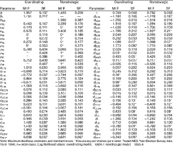
The coordinating and nonstrategic models produce similar results. Maximum-likelihood estimates (MLE) and standard errors (SE) for the parameters of the models, using observed attribute specifications (2a)–(2c), (5a)–(5c), and (6a)–(6c) are listed in Table 1.17
Over all years for the coordinating model, the percentage correctly classified by “predicting” for each observation the choice that has the highest probability using the parameter MLEs is 67.3% (by year, 64.2, 66.4, 68.2, 68.7, 66.7, and 70.1%), and the average probability of the choice actually made is 0.57 (by year, 0.54, 0.56, 0.58, 0.59, 0.56, and 0.59).
All the parameters that have the same interpretation in both models have statistically indistinguishable estimates. The MLEs for
cEC are near zero for every year except 1990, suggesting that for the most part retrospective economic evaluations do not affect choices between candidates.
18 The 95% confidence interval for cEC,90, computed as in Table 2, is (-0.001, 0.558).
Except for 1994, the MLEs for
dEC are statistically insignificant, so that retrospective evaluations also have no systematic effect on the choice not to vote. The MLEs for the party identification dummy variables show the familiar effects of party identification on candidate choices and turnout. The MLEs for
cDEM and
cREP point to a substantial incumbent advantage, while the MLEs for
dDEM and
dREP show that the probability of voting is lower when an incumbent is running for reelection. Greater subjective political efficacy, higher education, greater age, being married, and having lived longer at one's current residence all increase the loss from not voting and so increase the probability of voting. An elector who does not report at least one complete set of policy position values (γ
i = 0) is significantly more likely not to vote than an elector who does report policy positions. For 1994 and 1998, electors who have higher values of θ
i are significantly more likely to vote than electors who have lower values of θ
i: conservative electors were especially mobilized in those elections.
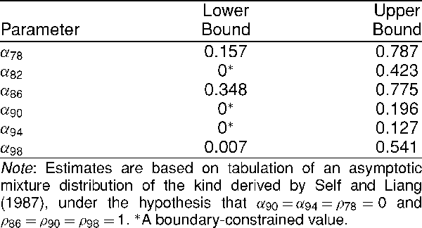
The coordinating model passes the tests of the conditions necessary for coordinating behavior. The LR test statistics for the constraint α = 1, imposed separately for each year, reject the constraint in every year.19
By year, the LR statistics −2(Lconstrained−L) and associated significance probabilities are 13.2 (p < 0.001), 35.2 (p < 0.0001), 12.0 (p < 0.01), 28.6 (p < 0.0001), 53.3 (p < 0.0001), and 26.7 (p < 0.0001). The significance probability is the upper-tail probability for the χ21 distribution under the null hypothesis α = 1, using the method of Davies (1987, Eq. 3.4) to adjust for the nuisance parameter ρ.
The 95% confidence intervals listed in
Table 2 support the same conclusions.
20 Table 1 shows α90, α94, ρ78, ρ86, ρ90, and ρ98 to have MLEs equal to either 0.0 or 1.0, on boundaries of the parameter space. We bootstrap (20,000 resamples) the score vectors of the MLEs in Table 1 to estimate the quantiles of the asymptotic distribution implied by the hypothesis that α90 = α94 = ρ78 = 0 and ρ86 = ρ90 = ρ98 = 1, which is a mixture of 64 censored multivariate normal distributions (Self and Liang 1987) and, hence, estimate the confidence intervals in Table 2.
Regarding the other conditions, 95% confidence intervals computed as in
Table 2 show
q (1.28, 1.81) and
bC (1.10, 1.90) to be positive and bounded well away from zero.
The MLEs for the nonstrategic model do not support the theory of nonstrategic institutional balancing. Only two of the six MLEs for α (
and
) are statistically distinguishable from zero;
. Rather than moderating, the estimates suggest that in most years electors are making direct choices between the parties' alternative policies.
While the log-likelihood of the coordinating model (−6824.7) is not much greater than that of the nonstrategic model (−6825.4), Vuong's (1989) overlapping models test nonetheless rejects the nonstrategic model as an alternative to the coordinating model. The MLEs and SEs in Table 1 clearly reject both bC = 0 and bNS = 0. Using the distribution of Vuong (1989, Eq. 6.4), the test statistic is n−1/2
(p < .0001).21
LRn = 16.50197 (Vuong 1989, Eq. 3.1) and
(Vuong 1989, Eq. 4.2). We compute both LRn and
with adjustments for sampling weights.
MODERATION, INSTITUTIONAL BALANCING, AND THE MIDTERM CYCLE
In the coordinating model, every elector anticipates a postelection policy that is intermediate between the parties' positions, unless α = 1. The coordinating model MLEs for α are less than 0.5 in every year except 1986 (see Table 1), suggesting that electors expected the president to be weaker than the House in determining postmidterm policy. The estimates for
show that the position of the House was expected to be closer to the Democratic position in 1978, 1982, 1986, and 1990 and closer to the Republican position in 1994 and 1998.22
By year,
and
computed using the parameter MLEs in Table 1 and 1978–1998 NES data are as follows: 0.393, 0.477; 0.437, 0.550; 0.418, 0.481; 0.373, 0.439; 0.544, 0.558; 0.524, and 0.455.
The systematic foundation for a midterm cycle in the coordinating model is that the equilibrium Republican House vote share each elector expects at the time of the presidential election is no longer an equilibrium once the identity of the president becomes known. The postelection disequilibrium decreases the probability that each elector votes for a House candidate of the president's party. The aggregation of such changes is the cycle-generating mechanism.
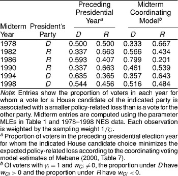
Does the coordinating model's moderating mechanism, which is based on λi, generate a midterm cycle? For a baseline measure of the effect policy-related incentives have on choices in the presidential election year preceding each midterm, we use Mebane's (2000, Table 7) estimates of the proportion of presidential-year voters for whom each combination of presidential and House choices would minimize expected policy-related losses.23
From Mebane's (2000) Table 7 coordinating model results we sum the percentages with choices RR and DR to get the percentage for whom choosing a Republican House candidate minimizes the expected policy-related loss, and we sum the percentages with choices DD and RD to get the percentages for whom choosing a Democrat minimizes the loss.
Consider the proportion of voters in a presidential election who would minimize their expected policy-related losses by voting for a House candidate of the same party as the new president. There is a policy-related foundation for a midterm cycle if that proportion is greater than the proportion of voters in the subsequent midterm who would minimize their policy-related losses by voting for a candidate of the same party as the president.
Table 3 shows that such a pattern occurs for all six midterm elections, although the decline from 1996 to 1998 is considerably smaller than for the other years.
24 By midterm year, the decreases shown in Table 3 are 0.167, 0.229, 0.206, 0.124, 0.278, and 0.028.
It is doubtful, however, whether most of the change in votes from presidential election to midterm is due purely to the postelection disequilibrium that the disappearance of uncertainty about the identity of the president brings about. Simulation using presidential-year NES data and Mebane's (2000) coordinating voting model suggests that immediately after the presidential election, due solely to the identity of the new president having become known, the equilibrium proportion of House votes for the new president's party typically falls by values ranging from about 0.01 to about 0.06.25
The simulation consists of recomputing the choice probabilities of Mebane's (2000) empirical coordinating model with
set equal to 0 or 1 depending on which party actually won the presidency in each election. By presidential year, 1976–1996, the losses for the new pre- sident's party are 0.011, 0.060, 0.015, 0.035, 0.043, and 0.058.
The simulated loss is substantially smaller than the corresponding decrease in policy-related support for the president's party shown in
Table 3 for each midterm year except 1998. Other factors that change between the presidential and the midterm elections are modulating the magnitude of the policy-related midterm losses. Such factors include the fact that the president is usually expected to have less influence on policy after midterm than after the preceding presidential election.
26 The upper bounds of the 95% confidence intervals for α, in Table 2, are smaller than the lower bounds of the 95% confidence intervals that Mebane (2000, Table 4) reports for αD or αR for the winning presidential candidate for all years except 1984. The interval for αR,84, (0.34, 0.79), is virtually the same as the interval for α86 in Table 2, suggesting that voters believed that Reagan's influence on policy remained about the same throughout his second term.
The form of each elector's evaluation of the policy-related losses also changes: at midterm an elector's evaluation of λ
i does not depend on the elector's retrospective evaluation of the economy, as it does in presidential election years.
27 And between elections parties may change their policy positions, or voters may change their ideal points, and substantively different policies come into play.
SURGE AND DECLINE
The theory of surge and decline suggests a possible reason for the relationship between voters' most preferred policies and the policy positions they attribute to the parties to change in a systematic way between the presidential and the midterm elections. According to the theory, during the heightened mobilization of presidential elections more electors with marginal political involvement turn out to vote than during midterm elections, and this group disproportionately votes for the party of the winning presidential candidate (Campbell 1966). Campbell's (1987) revised theory treats midterm as a return to a normal partisan vote, less influenced by short-run concerns than the presidential election. He writes, “Surge of interest and information in presidential elections will affect the turnout of peripheral partisans and the vote choice of independents” (p. 968). Born (1990, 642, note 30) raises serious doubts about those revisions.
Perhaps the surge of marginal electors who, according to the theory, vote for House candidates of the same party as the presidential winner do so because they like that party's policy position better than the other party's policy position. The posited midterm decline in their turnout should have two major effects. On average, midterm voters should tend to have policy ideal points that are farther from the president's party than presidential-year voters do, and midterm nonvoters should tend to have policy ideal points that are closer to the president's party than presidential-year nonvoters do. We show that NES data from the elections of 1976 through 1998 do not support the existence of such a surge and decline mechanism.
For most electors, turnout at midterm is only weakly related to expected policy-related losses. In the empirical coordinating model, the policy-related loss expected by elector i affects the probability that i does not vote (μi,A) via wCi. We assess the effect that policy-related losses have on midterm turnout by computing the effect on μi,A of setting wCi = 0 for each i in the midterm NES data. By midterm year, 1978–1998, the median differences between μi,A using the original wCi value and μi,A with wCi = 0 are -0.0000017, −0.0017, −0.00047, −0.0014, −0.0018, and −0.0011.28
The medians include only observations that have γi = 1.
The median differences always have a smaller magnitude for Independents than for other electors.
29 For Independent Independents the medians are 0, −0.00003, 0, 0, −0.00002, and −0.00041.
Such small effects will usually be dominated by other factors, such as partisanship per se, that much more strongly affect the probability of not voting.
Nonetheless it may be that midterm voters see themselves as farther from the president's party on policy than presidential-year voters do, while midterm nonvoters see themselves as closer to the policy of the presidential winner's party than do presidential-year nonvoters. To compare the policy proximities, we use the coordinating model parameter estimates of Mebane (2000) to compute ideal points (θi) and party policy positions (θDi and θRi) for both voters and nonvoters in the NES data for each presidential election year from 1976 through 1996. We define a voter to be anyone who reports having voted for either the Democrat or the Republican in the House race and a nonvoter to be anyone who does not report such a vote. We include only those who report at least one complete set of policy position values.30
Voters and nonvoters by year are as follows: 982, 887; 802, 551; 1,099, 617; 940, 725; 1,244, 841; and 996, 600.
For each elector
i we compute the absolute difference between i's ideal point and the position of the party that won the presidential election. The absolute difference is |θ
i−θ
Di| if the Democrat won the election and |θ
i−θ
Ri| if the Republican won.
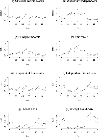
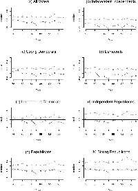
Each panel in Fig. 1 displays for each year the median of the absolute differences for a different set of electors. Figure 1a shows the medians for all voters and nonvoters, and the remaining panels show the medians for each of the seven NES types of party identifiers. Among all voters (Fig. 1a) the median absolute difference between each voter's ideal point and the position the voter attributes to the presidential winner's party is always greater at midterm than it is during the preceding presidential election year. But in every case except 1992–1994, the median absolute difference is also greater at midterm among all nonvoters. The pattern among nonvoters does not match what surge and decline theory predicts.
The closest match to the pattern predicted by the surge and decline theory occurs among Independent Independents (Fig. 1b), but even there the support for surge and decline is weak at best. In 1978, 1990, and 1994 there are decreases at midterm in the median absolute difference among nonvoters. But in the remaining three midterms the median absolute difference increases from the preceding presidential year among nonvoters. Moreover, in 1990 the median absolute difference decreases among voters. There is hardly any support for surge and decline in the data for Independent Democrats and Independent Republicans (Figs. 1e and 1f). Among nonvoters there are nine instances where the median absolute difference increases at midterm and only three instances where it decreases at midterm. Moreover, among Independent Democrats there are two instances (1990 and 1998) where the median absolute difference for voters decreases at midterm and among Independent Republicans there is one instance (1998).
Instead of the pattern that the surge and decline theory predicts, what we see is that typically both voters and nonvoters are farther from the policy of the president's party at midterm than they were at the time that the party won the presidency in the preceding election. Nonvoters are somewhat more likely than voters are to be closer to the president's party at midterm, but the difference is not regular enough for surge and decline to be a compelling explanation.
Surge and decline theory also asserts that some regular voters deviate from their partisan affiliation during the presidential elections and vote for House candidates of the presidential winner's party, but return to their normal partisan vote at midterm (Born 1990, 635). The insignificant effects (cEC) we estimate retrospective economic evaluations have on choices between candidates may partly account for that. In Mebane (2000), the corresponding parameters (cH1) are significant in four of the six presidential years. Presidential-year deviations prompted by economic evaluations tend to disappear at midterm.
MODERATION BY CHANGES IN POLICY POSITIONS
Figure 1 shows that the absolute difference between electors' ideal points and the policy positions of the party that won the presidential election usually increases at midterm. Figure 1 is a bit one-sided, however, because it summarizes the relationship between electors' ideal points and only one party's policy positions, but the expected policy-related losses that affect vote choices depend on both parties' policies.
To assess the components of change it is important to consider not merely the magnitudes but also the directions in which the aggregate of voters moves with respect to the parties. Consider a situation in which all voters think the Democratic party policy position is left of the Republican party position, i.e., θDi < θRi for all voters i. We may characterize the aggregate movement across elections in terms of two median statistics: the median difference between ideal points and Democratic positions, denoted med_i(θi − θDi), and Republican positions, denoted medi(θi − θRi). Let ΔD = medMi(θi−θDi) − medPi(θi−θDi) denote the difference between the median policy difference with respect to the Democratic party at midterm and the median difference in the preceding presidential year. If ΔD < 0, then at midterm voters have ideal points more to the left of the positions they attribute to the Democratic party than in the preceding presidential year and, other things equal, a greater proportion vote for Democratic candidates at midterm than in the preceding presidential year. If ΔD > 0, then midterm voters have ideal points more to the right of Democratic party positions, and a smaller proportion vote for Democratic candidates at midterm. Analogously let ΔR = medMi(θi−θRi) − medPi(θi−θRi) denote the difference between midterm and the preceding presidential year of the policy differences with respect to the Republican party. If ΔR > 0, then midterm voters have ideal points more to the right of Republican party positions, and Republican candidates receive a greater proportion of votes at midterm than in the preceding presidential year. If ΔR < 0, then Republican candidates receive a smaller proportion of votes at midterm. Because θi, θDi, and θRi vary independently, all combinations of positive and negative values for ΔD and ΔR are possible.
Of particular interest are circumstances in which ΔD and ΔR are either both positive or both negative. If ΔD > 0 and ΔR > 0, then between elections the distribution of voters' ideal points has moved to the right relative to both parties' positions. Other things equal, Republican House vote share
increases. If a Democrat is president, the result is a kind of policy moderation: policy outcomes are expected to be closer to the midterm Republican position.31
This assumes that α does not increase after midterm (recall footnote 26).
If Δ
D < 0 and Δ
R < 0, then between elections the distribution of voters' ideal points has moved to the left relative to both parties' positions, the Republican House vote share decreases, and if a Republican is president, there is moderation of expected policy toward the midterm Democratic position.
Moderation via such a pattern of changes occurs in five of the six midterm elections from 1978 through 1998, according to NES data. Using NES data to compute the median differences between ideal points and the parties' positions, it is necessary to adjust for the fact that some voters place the Democratic party policy position to the right of the Republican party position: for some voters, θDi > θRi. Because moderation refers to movement from one party toward the other and does not depend on the orientation with which each voter interprets its ideal point and the parties' positions, we use the sign of the difference between θRi and θDi to orient all voters the same way. We compute medMi[(θi − θDi) sgn (θRi − θDi)] and medMi[(θi − θRi) sgn(θRi − θDi)] for each midterm year and analogous quantities for each presidential year. In Fig. 2 we plot the values for all voters who report at least one complete set of policy position values (as in Fig. 1) and, in separate panels, for party identifier subsets. The interelection differences are now:
The sign of each ΔD and ΔR value is indicated by the slope of the line that joins each presidential-year median to the succeeding midterm median.
Figure 2a shows that among all voters, in every midterm except 1998 there is moderation based on interelection changes in the location of voters' ideal points relative to the parties' positions.32
The pattern of changes is similar among nonvoters.
In 1978 and 1994, with Democratic presidents, we have Δ
D > 0 and Δ
R > 0, and in 1982, 1986, and 1990, with Republican presidents, we have Δ
D < 0 and Δ
R < 0. In 1998 there is a Democratic president but nonetheless Δ
D < 0 and Δ
R < 0: Democrats' House vote share was pushed up, because between 1996 and 1998 the distribution of voters' ideal points shifted to the left relative to both parties' positions. The pattern of interelection changes is similar across all of the partisan subsets and within each subset is by and large similar to the pattern among all voters, except for 1988–1990. Between 1988 and 1990 we have Δ
R < 0 among all voters but within each partisan subset Δ
R > 0. The reason for the difference is that a higher proportion of voters identified as Democrats and a lower proportion as Republicans in 1990 than in 1988,
33 In 1988 the proportions identifying as Strong Democrats, Democrats, Republicans, and Strong Republicans were 0.20, 0.16, 0.14, and 0.20. In 1990 the proportions were 0.28, 0.18, 0.14, and 0.14.
and (θ
i − θ
Ri) sgn (θ
Ri − θ
Di) is more negative among Democratic voters than among Republican voters.
The moderating pattern associated with having either a Democratic president, ΔD > 0 and ΔR > 0, or a Republican president, ΔD < 0 and ΔR < 0, differs from the mechanism of disappearing uncertainty, but the fluctuations in policy positions may relate to the idea that parties may commit to policies different from their ideal policies. Alesina and Rosenthal (1995, 127–36) report that in such an extension of their model parties often announce policies that are more polarized than their ideal policies are. Polarization increases as the president's power (α) falls. As we mentioned previously, voters usually believe that the president will be more powerful before midterm than afterward. Alesina and Rosenthal (1995) do not examine models in which α changes at midterm, but we may speculate that—with the parties possibly changing their positions at midterm—there would be a tendency for polarization to increase at midterm.
The NES data from 1976 through 1998 support the idea that polarization is greater at midterm. Among voters, the median absolute difference between the parties' positions is smaller in the presidential election than at midterm in five of the six pairs of elections (the exception is 1988–1990).34
By pairs of elections, the medi|θRi − θDi| values are as follows: 1976–1978, 0.20 and 0.21; 1980–1982, 0.33 and 0.39; 1984–1986, 0.36 and 0.45; 1988–1990, 0.33 and 0.29; 1992–1994, 0.37 and 0.41; and 1996–1998, 0.34 and 0.36.
The interelection changes in the median absolute differences are, however, small compared to the observed magnitudes of Δ
D and Δ
R. These results are only suggestive because by construction our measures of party positions are within the unit interval [0, 1] in every year.
The changes ΔD and ΔR may also arise because voters learn something after the presidential election. They may learn more about what a party's true policy position is, about a policy position's consequences, or about elected officials' competence to implement the policy. Any of these may be a reason for a voter to update the relationship between the voter's ideal point and the positions the voter attributes to the parties. A party's actions either in the presidency or in Congress may be informative. Perhaps, for instance, the Democrat-favoring changes shown in Fig. 2 for 1996 to 1998 stem from judgments that Republicans in the House were especially incompetent or extreme.35
The July 1997 plot to remove Newt Gingrich as Speaker revealed disarray among the Republican House leadership. Gingrich resigned shortly after the 1998 election. Polls during 1998 showed that most voters disliked the Republican effort to impeach the president (e.g., Pew Research Center 1998).
The unanswered question is, Why are movements away from the president's party more typical. Why do electors not learn more often that the president's party is more competent or less extreme than they previously thought?
One of the difficulties of explaining why moderation by policy position changes occurs is that our policy position measures are based on the gaps between electors' ideal points and the perceived positions of the two major parties. Across elections, we cannot distinguish between movement in electors' ideal points and movement in the positions of the political parties. For example, notwithstanding the polarization argument, it is possible that a party in office follows policies more extreme than it proposed at election time. Electors may learn this and consequently the gap between the president's party and the electors increases at midterm because electors' perceptions of the parties change. With our data we cannot distinguish such a pattern from one in which electors change their ideal points because they learn more about policies' consequences.
Moderation by policy position changes may explain the pattern that was the original focus of the negative voting variant of surge and decline. Beyond turnout and coattails effects, there is an additional midterm loss apparently due to “public disappointments with the incumbent presidential party's performance” (Campbell 1991, 483). Tufte (1975) measures this phenomenon by a decline in presidential approval that usually occurs in the first two years of an administration. Born (1990, Table 4) measures the same phenomenon by changes in feeling thermometer scores. The usual pattern of interelection changes in policy positions would cause such changes in approval and in feeling thermometers.
CONCLUSION
The NES data strongly confirm the strategic theory of policy moderation. The estimated parameters of the coordinating model satisfy all of the conditions necessary to describe coordinating behavior. The nonstrategic model fails to describe policy-moderating behavior and fits the data significantly worse than does the coordinating model. Coordination also affects decisions whether to vote, but the effects on turnout probabilities are typically small.
Midterm loss is in part caused by policy moderation that occurs because uncertainty about which party will control the presidency disappears after the presidential election. But the mechanism of disappearing uncertainty does not itself explain why midterm losses are as large as they are nor why midterm losses occur as frequently as they do.
The largest source of loss of support for the president's party at midterm is a regularly repeated pattern in which by midterm the median differences between voters' ideal points and the parties' policy positions have become less favorable for the president's party than they were at the time of the presidential election (the same pattern occurs among nonvoters). Such a pattern occurs in all five of the interelection periods during 1976–1998 after which the president's party suffered a midterm loss. Between 1996 and 1998 the pattern reverses: The distribution of voters' ideal points and party positions becomes more favorable to the Democratic party notwithstanding the fact that Democrat Bill Clinton is president, to such an extent that on the whole the Democrats enjoyed a small midterm gain in 1998.
The policies involved in the interelection changes are not limited to macroeconomic policy. Indeed, only in 1980 do the NES survey items we use to measure ideal points and party positions include scales that refer to macroeconomic policy. The interelection changes we document involve a wide range of policies, and the composition of the set of policies changes over time. Nonetheless, changes go in the same direction—away from the president's party—during five of the six interelection periods our data cover. Why the changes typically cut against the president's party is not clear. The dynamic is not explained by variations in turnout.
Our finding that strategic coordination exists shows that the reach of the incentives the constitutional separation of powers creates extends beyond officials to electors. The separation of powers causes electors to attend to one another and make choices that help produce moderate policy outcomes. It is important to keep clear that in moderation via noncooperative coordinating equilibrium, no one has a taste for moderation per se. It is not that coordinating electors are committed to divided government because of a sincere commitment to “cognitive Madisonianism” (Ladd 1990, 67; Sigelman et al. 1997). Each elector always most prefers his or her own ideal point. Moderation occurs only as a collective outcome due to electors' mutual strategic adjustments.






Comments
No Comments have been published for this article.