1 Introduction
Since the earlier experimental studies by Laufer (Reference Laufer1951) and Comte-Bellot (Reference Comte-Bellot1963), the fully developed turbulent channel flow has received a great deal of attention, both experimentally and numerically, due mainly to the simplicity of the flow geometry and consequent simplifications that can be made to the governing equations of motion. A major stimulus for unravelling various aspects of the physics of turbulence, especially close to the wall, was provided by the direct numerical simulation (DNS) of Kim, Moin & Moser (Reference Kim, Moin and Moser1987) in which the governing equations were solved directly so that all the essential scales of the motion were resolved. In their DNS, the data were obtained at a relatively small value (
 $=$
180) of the Kármán number
 $h^{+}$
(
 $\equiv U_{{\it\tau}}h/{\it\nu}$
), which represents the ratio of the half-width of the channel
 $h$
and the viscous length scale
 ${\it\nu}/U_{{\it\tau}}$
(
 $U_{{\it\tau}}(\equiv ({\it\tau}_{w}/{\it\rho})^{1/2})$
is the friction velocity, where
 ${\it\tau}_{w}$
is the wall shear stress and
 ${\it\rho}$
is the density of the fluid; the superscript
 $+$
will subsequently denote normalization by
 ${\it\nu}/U_{{\it\tau}}$
and
 $U_{{\it\tau}}$
). Since then, many DNSs (e.g. Moser, Kim & Mansour Reference Moser, Kim and Mansour1999; Abe, Kawamura & Matsuo Reference Abe, Kawamura and Matsuo2001, Reference Abe, Kawamura and Matsuo2004a
; Iwamoto, Suzuki & Kasagi Reference Iwamoto, Suzuki and Kasagi2002; Abe, Kawamura & Choi Reference Abe, Kawamura and Choi2004b
; del Álamo et al.
Reference del Álamo, Jiménez, Zandonade and Moser2004; Tanahashi et al.
Reference Tanahashi, Kang, Miyamoto, Shiokawa and Miyauchi2004; Hu, Morfey & Sandham Reference Hu, Morfey and Sandham2006; Laadhari Reference Laadhari2007; Hoyas & Jiménez Reference Hoyas and Jiménez2008; Abe, Antonia & Kawamura Reference Abe, Antonia and Kawamura2009; Bernardini, Pirozzoli & Orlandi Reference Bernardini, Pirozzoli and Orlandi2014; Lozano-Durán & Jiménez Reference Lozano-Durán and Jiménez2014; Vreman & Kuerten Reference Vreman and Kuerten2014; Lee & Moser Reference Lee and Moser2015) have been performed at increasingly larger values of
 $h^{+}$
in the same flow. To date, the maximum value for
 $h^{+}$
reached in the DNS of the present flow is 5000 (Lee & Moser Reference Lee and Moser2015) without compromising spatial resolution requirements. This is about a factor of 2 smaller than the maximum value achieved in the laboratory by Comte-Bellot (Reference Comte-Bellot1963) by using a large physical value of
 $h$
(
 $=$
0.09 m).
A major difficulty in experiments is the accurate determination of the wall shear stress
 ${\it\tau}_{w}$
. In this context, significant attention has been given to the streamwise length (
 $L$
) and the aspect ratio (AR) of the channel. To achieve a fully developed flow with
 $\text{d}\bar{P}/\text{d}x=\text{const.}$
, a relatively long channel is required (Monty (Reference Monty2005) suggests
 $L=260h$
). The AR also needs to be as large as possible to avoid possible side wall effects and hence ensure two-dimensionality (Monty (Reference Monty2005) suggests that the AR should be at least 12). When these requirements are met, the momentum balance over a control volume which extends across the whole section of the channel and includes the two walls yields
 $$\begin{eqnarray}{\it\tau}_{w}=-h\frac{\text{d}\bar{P}}{\text{d}x}.\end{eqnarray}$$
However, in order to check that momentum is conserved on an integral basis, an independent, preferably direct estimate of
 ${\it\tau}_{w}$
is needed. Zanoun, Durst & Nagib (Reference Zanoun, Durst and Nagib2003) have estimated
 ${\it\tau}_{w}$
using both the measured pressure gradient and the oil film interferometry technique in a fully developed channel flow. Good agreement between the two estimates was obtained for values of
 $h^{+}$
extending up to
 $h^{+}\approx 5000$
. The corresponding data for the skin friction coefficient defined as
 $$\begin{eqnarray}C_{f}\equiv {\it\tau}_{w}/{\textstyle \frac{1}{2}}{\it\rho}U_{b}^{2}=2/U_{b}^{+2}\end{eqnarray}$$
(
 $U_{b}$
is the bulk mean velocity defined in the channel as
 $U_{b}\equiv (1/h)\int _{0}^{h}\bar{U}\,\text{d}y$
) were consistent with Dean’s (Reference Dean1978) well-known power-law formulation as a function of
 $Re_{b}$
(
 $\equiv U_{b}2h/{\it\nu}$
), viz.
 $$\begin{eqnarray}C_{f}=0.073Re_{b}^{-1/4}.\end{eqnarray}$$
Recently, Zanoun, Nagib & Durst (Reference Zanoun, Nagib and Durst2009) observed that the logarithmic skin friction relation
 $$\begin{eqnarray}U_{b}^{+}=\frac{1}{{\it\kappa}}\ln (h^{+})-\frac{1}{{\it\kappa}}+A\end{eqnarray}$$
or, equivalently,
 $$\begin{eqnarray}\sqrt{\frac{2}{C_{f}}}=\frac{1}{{\it\kappa}}\ln \left(Re_{b}\sqrt{C_{f}}/2\sqrt{2}\right)-\frac{1}{{\it\kappa}}+A\end{eqnarray}$$
obtained from the logarithmic law of the wall
 $$\begin{eqnarray}U^{+}=\frac{1}{{\it\kappa}}\ln (y^{+})+A\end{eqnarray}$$
(
 ${\it\kappa}$
and
 $A$
denote the Kármán constant and the additive constant, respectively), with
 ${\it\kappa}=0.37$
and
 $A=3.7$
, as obtained by Zanoun et al. (Reference Zanoun, Durst and Nagib2003), represents more accurately the experimental skin friction data than Dean’s (Reference Dean1978) formula (1.3), in particular, for
 $h^{+}>2000$
(see figure 5 of their paper). Relation (1.4) is obtained by integrating (1.6) across the channel. Although this may be valid strictly when
 $h^{+}\rightarrow \infty$
, the mean velocity profiles of Zanoun et al. (Reference Zanoun, Durst and Nagib2003) do not deviate significantly from the log law over a wide cross-section of the flow (this was also confirmed by Monty et al. (Reference Monty, Stewart, Williams and Chong2007)). More recently, Schultz & Flack (Reference Schultz and Flack2013) made laser Doppler velocimetry measurements in the range
 $h^{+}=1000{-}6000$
and employed (1.1) to determine
 ${\it\tau}_{w}$
. They reported that the logarithmic friction relation (1.4) with
 ${\it\kappa}=0.40$
and
 $A=5.0$
provides a good fit to their experimental data.
An interesting question which arises from the above observations is why a skin friction relation, based on log-law constants which can only be defined, with some degree of confidence, for
 $h^{+}>2000$
, represents adequately data at values of
 $h^{+}$
that are smaller by almost one order of magnitude. For example, for the
 $h^{+}=180$
DNS channel data of Kim et al. (Reference Kim, Moin and Moser1987),
 $C_{f}$
is approximately 8 % smaller than the prediction by the logarithmic skin friction law (1.5). It is also only approximately 3 % smaller than the value given by Dean’s (Reference Dean1978) relation (1.3) (see also figure 1 of Abe et al. (Reference Abe, Kawamura and Matsuo2001)). We explore this theme by focusing almost exclusively on the behaviour of the turbulent dissipation rate; this approach provides an answer to the question raised above. Particular attention is given to the energy dissipation function
 $E$
(Rotta Reference Rotta1962) since
 $E/U_{{\it\tau}}^{3}$
is equal to
 $U_{b}^{+}$
. This latter relation is obtained readily by considering that the total energy dissipated in the channel is equal to the energy input via the mean pressure gradient, viz.
 $$\begin{eqnarray}E=-\frac{1}{{\it\rho}}\frac{\text{d}\bar{P}}{\text{d}x}U_{b}h=U_{{\it\tau}}^{2}U_{b}\quad \text{or equivalently},\quad U_{b}^{+}=E/U_{{\it\tau}}^{3}.\end{eqnarray}$$
Possible relations for
 $U_{b}^{+}$
are therefore obtained on the basis of not only the velocity log law (viz. (1.4)), but also via
 $E$
(viz. (1.7)). This approach provides an interesting insight into the logarithmic skin friction law since the logarithmic
 $h^{+}$
dependence of
 $U_{b}^{+}$
appears to be established at lower Reynolds numbers than the velocity log law. In this context, Laadhari (Reference Laadhari2007) examined the relative contributions of the turbulent strain rate
 $\overline{{\it\varepsilon}}$
and that which arises from the mean strain rate
 $\overline{{\it\varepsilon}}_{mean}$
, viz.
 $$\begin{eqnarray}E\equiv \underbrace{{\it\nu}\overline{u_{i,j}(u_{i,j}+u_{j,i})}}_{\overline{{\it\varepsilon}}}+\underbrace{{\it\nu}\overline{U}_{i,j}(\overline{U}_{i,j}+\overline{U}_{j,i})}_{\overline{{\it\varepsilon}}_{mean}}.\end{eqnarray}$$
Note that
 $u_{1}$
,
 $u_{2}$
,
 $u_{3}$
denote the streamwise, wall-normal and spanwise velocity fluctuations, respectively;
 $u$
,
 $v$
,
 $w$
are used interchangeably with
 $u_{1}$
,
 $u_{2}$
,
 $u_{3}$
;
 ${\it\nu}$
denotes the kinematic viscosity and the overbar denotes averaging with respect to
 $x$
,
 $z$
(
 $x$
,
 $y$
,
 $z$
are the streamwise, wall-normal and spanwise directions, respectively) and
 $t$
(time); upper cases denote instantaneous quantities. He noted that the logarithmic friction relation is obtained from
 $E$
, with
 ${\it\kappa}=0.38$
and
 $A=4.65$
, and the resulting relation agrees well with his DNS data for
 $h^{+}>500$
as well as the higher
 $h^{+}$
data of Zanoun et al. (Reference Zanoun, Durst and Nagib2003). In the present paper, we extend Laadhari’s (Reference Laadhari2007) work and assess how
 $E$
varies over a wider range of
 $h^{+}$
than covered by Laadhari (Reference Laadhari2007). In particular, we try to clarify how the logarithmic dependence of
 $U_{b}^{+}$
is established by focusing on how the turbulent energy dissipation rate
 $\overline{{\it\varepsilon}}$
scales in different regions of the channel. We also give significant attention to the overlap scaling of
 $\overline{{\it\varepsilon}}$
by applying a matching argument to elucidate the outer layer similarity we observe for
 $\overline{{\it\varepsilon}}$
.
This paper is organized as follows. In § 2,
 $E$
is explained in the context of a turbulent channel flow. A brief description is given in § 3 of the present DNS databases for the channel flow. The effect of the streamwise domain on
 $E$
is addressed in § 4.1. Results for the dependence of
 $E$
on
 $h^{+}$
are presented in § 4.2 together with available DNS and experimental data. Section 4.3 extends the
 $U_{b}^{+}$
relation established in § 4.2 to a pipe flow since (1.7) holds in internal flows. The relationship between the resulting
 $\ln (h^{+})$
dependence of
 $U_{b}^{+}$
and the scaling law of the turbulent energy dissipation rate is also discussed in some detail in §§ 4.4 and 4.5 where comparisons are made with available DNS data of
 $\overline{{\it\varepsilon}}$
for the pipe and the zero-pressure-gradient turbulent boundary layer. Conclusions are given in § 5.
2 Relation for the energy dissipation function
 $E$
in a channel flow

Rotta (Reference Rotta1962) discussed the energy dissipation function
 $E$
in some detail in the context of the boundary layer. By integrating the transport equations of the mean and turbulent kinetic energy between the wall and the freestream, he obtained
 $$\begin{eqnarray}\displaystyle E & = & \displaystyle \int _{0}^{\infty }\overline{{\it\varepsilon}}\,\text{d}y+\int _{0}^{\infty }{\it\nu}\left(\frac{\partial \overline{U}}{\partial y}\right)^{2}\,\text{d}y\nonumber\\ \displaystyle & = & \displaystyle \int _{0}^{\infty }\frac{{\it\tau}}{{\it\rho}}\left(\frac{\partial \overline{U}}{\partial y}\right)\,\text{d}y-\int _{0}^{\infty }\left(\overline{u^{2}}-\overline{v^{2}}\right)\frac{\partial \overline{U}}{\partial x}\,\text{d}y-\frac{\text{d}}{\text{d}x}\int _{0}^{\infty }\overline{U}k\,\text{d}y,\end{eqnarray}$$
where
 ${\it\tau}$
is the total shear stress and
 $k$
the turbulent kinetic energy. Rotta (Reference Rotta1962) underlined that the last two terms on the right of (2.1) are merely corrections and that the main contribution to
 $E$
comes from the work done by the shear stress.
In a channel flow, a relation for
 $E$
is obtained readily using the total shear stress relation, viz.
 $$\begin{eqnarray}\frac{{\it\tau}}{{\it\rho}}\equiv -\overline{uv}+{\it\nu}\frac{\text{d}\bar{U}}{\text{d}y}=\frac{1}{{\it\rho}}\left({\it\tau}_{w}-y\frac{\text{d}\bar{P}}{\text{d}x}\right),\end{eqnarray}$$
where the mean-pressure-gradient term appears. By multiplying (2.2) by
 $\text{d}\overline{U}/\text{d}y$
, we obtain the energy balance for the mean flow, viz.
 $$\begin{eqnarray}-\!\overline{uv}\frac{\text{d}\bar{U}}{\text{d}y}+{\it\nu}\left(\frac{\text{d}\bar{U}}{\text{d}y}\right)^{2}=\frac{1}{{\it\rho}}\left({\it\tau}_{w}\frac{\text{d}\bar{U}}{\text{d}y}-y\frac{\text{d}\bar{P}}{\text{d}x}\frac{\text{d}\bar{U}}{\text{d}y}\right).\end{eqnarray}$$
 $({\it\tau}_{w}/{\it\rho})(\text{d}\overline{U}/\text{d}y)$
represents the rate of energy transfer from the outer part of the boundary layer to the inner region (see also DeGraaff & Eaton Reference DeGraaff and Eaton2000; Morrison et al.
Reference Morrison, McKeon, Jiang and Smits2004); the term which includes
 $\text{d}\overline{P}/\text{d}x$
is the energy input from the mean pressure gradient. The energy is partly dissipated directly by viscosity (the second term on the left-hand side of (2.3)) and partly extracted to turbulence via the work done by the Reynolds shear stress (the first term on the left-hand side of (2.3)).
By assuming the symmetry with respect to the centreline, the integral of (2.3) from
 $y=0$
to
 $h$
then leads to
 $$\begin{eqnarray}\int _{0}^{h}-\overline{uv}\frac{\text{d}\bar{U}}{\text{d}y}\,\text{d}y+\int _{0}^{h}{\it\nu}\left(\frac{\text{d}\bar{U}}{\text{d}y}\right)^{2}\,\text{d}y=-\frac{1}{{\it\rho}}\frac{\text{d}\bar{P}}{\text{d}x}\int _{0}^{h}\bar{U}\,\text{d}y,\end{eqnarray}$$
or equivalently,
 $$\begin{eqnarray}\langle \overline{{\it\varepsilon}}\rangle +\left\langle {\it\nu}\left(\frac{\text{d}\bar{U}}{\text{d}y}\right)^{2}\right\rangle =U_{{\it\tau}}^{2}U_{b},\end{eqnarray}$$
where the angular brackets denote integration with respect to
 $y$
across the channel half-width. Note that in (2.5) we also consider the energy balance for the turbulent kinetic energy so that
 $\langle P_{k}\rangle$
is replaced by
 $\langle \overline{{\it\varepsilon}}\rangle$
where
 $P_{k}\equiv -\overline{uv}(\text{d}\bar{U}/\text{d}y)$
since the relation
 $$\begin{eqnarray}\langle P_{k}\rangle =\langle \overline{{\it\varepsilon}}\rangle ,\end{eqnarray}$$
which expresses equality between the net turbulent energy production and the total turbulent energy dissipation rate, holds in a channel flow. Relation (2.5) can then be arranged as follows
 $$\begin{eqnarray}\frac{U_{b}}{U_{{\it\tau}}}=\frac{\langle \overline{{\it\varepsilon}}\rangle }{U_{{\it\tau}}^{3}}+\left.\left\langle {\it\nu}\left(\frac{\text{d}\bar{U}}{\text{d}y}\right)^{2}\right\rangle \right/U_{{\it\tau}}^{3}=\frac{E}{U_{{\it\tau}}^{3}}.\end{eqnarray}$$
Equation (2.7) is equivalent to the relationship between
 $E/U_{{\it\tau}}^{3}$
and
 $U_{b}/U_{{\it\tau}}$
, (1.7). The viscous contribution is expected to dominate near the wall while the contribution from the turbulent energy dissipation rate should dominate elsewhere. It is also expected that the viscous term will be dominant at small
 $h^{+}$
whereas
 $\langle \overline{{\it\varepsilon}}\rangle$
should become increasingly important as
 $h^{+}$
becomes very large so that the
 $h^{+}$
dependence of
 $U_{b}/U_{{\it\tau}}$
, which is related to the skin friction coefficient
 $C_{f}\equiv 2(U_{{\it\tau}}/U_{b})^{2}$
(1.2), should essentially reflect that of the normalized integrated energy dissipation rates across the channel.
3 DNS databases
The present numerical databases have been obtained from DNSs in a turbulent channel flow with passive scalar transport by Abe et al. (Reference Abe, Kawamura and Matsuo2004a
, Reference Abe, Antonia and Kawamura2009). In the present study, we exclusively use flow field data for a fully developed turbulent channel flow driven by a constant streamwise mean pressure gradient. Four values of
 $h^{+}$
(
 $=180$
, 395, 640 and 1020) are used. We also consider other DNS data available in the literature up to
 $h^{+}=5200$
(Moser et al.
Reference Moser, Kim and Mansour1999; Iwamoto et al.
Reference Iwamoto, Suzuki and Kasagi2002; del Álamo et al.
Reference del Álamo, Jiménez, Zandonade and Moser2004; Tanahashi et al.
Reference Tanahashi, Kang, Miyamoto, Shiokawa and Miyauchi2004; Tsukahara et al.
Reference Tsukahara, Seki, Kawamura and Tochio2005; Hu et al.
Reference Hu, Morfey and Sandham2006; Laadhari Reference Laadhari2007; Hoyas & Jiménez Reference Hoyas and Jiménez2008; Bernardini et al.
Reference Bernardini, Pirozzoli and Orlandi2014; Lozano-Durán & Jiménez Reference Lozano-Durán and Jiménez2014; Vreman & Kuerten Reference Vreman and Kuerten2014; Lee & Moser Reference Lee and Moser2015).
The numerical methodology for the DNSs is briefly as follows. A fractional step method is used with semi-implicit time advancement. The third-order Runge–Kutta method is used for the viscous terms in the
 $y$
direction and the Crank–Nicolson method is used for the other terms. A finite difference method is adopted for the spatial discretization. A fourth-order central scheme is used in the
 $x$
and
 $z$
directions, whilst a second-order central scheme is used in the
 $y$
direction. The periodic boundary condition is employed in the
 $x$
and
 $z$
directions, whereas the no-slip condition applies in the
 $y$
direction. Further details of the simulations are given in Abe et al. (Reference Abe, Kawamura and Matsuo2001, Reference Abe, Kawamura and Matsuo2004a
,Reference Abe, Kawamura and Choi
b
, Reference Abe, Antonia and Kawamura2009) and Antonia, Abe & Kawamura (Reference Antonia, Abe and Kawamura2009), and the reader may refer to these papers for information on basic turbulence statistics.
Domain size, grid points and spatial resolution of the DNS databases.

The computational domain size (
 $L_{x}\times L_{y}\times L_{z}$
), number of grid points (
 $N_{x}\times N_{y}\times N_{z}$
) and spatial resolution (
 ${\rm\Delta}x$
,
 ${\rm\Delta}y$
,
 ${\rm\Delta}z$
) are given in table 1, the superscript
 $^{\ast }$
representing normalization by either
 $v_{K}$
(
 $\equiv ({\it\nu}\overline{{\it\varepsilon}})^{1/4}$
; the Kolmogorov velocity scale) or
 ${\it\eta}$
(
 $\equiv ({\it\nu}^{3}/\overline{{\it\varepsilon}})^{1/4}$
; the Kolmogorov length scale); the subscripts
 $w$
and
 $c$
referring to the wall and centreline, respectively. The effect of the domain size was examined by Abe et al. (Reference Abe, Kawamura and Choi2004b
) (
 $h^{+}=640$
) who compared two cases:
 $(L_{x}\times L_{z})=(6.4h\times 2h)$
and (
 $12.8h\times 6.4h$
). They found that the effect on the mean flow variables and second-order moments was negligible. They also examined one-dimensional energy spectra and noted that their streamwise domain size was not large enough to include all the large-scale contributions, whereas their spanwise domain size was quite sufficient. Abe et al. (Reference Abe, Kawamura and Choi2004b
) also reported that the most energetic spanwise wavelength of
 $u$
is approximately 1.3–
 $1.6h$
in the outer region. The identical behaviour was also observed for
 $h^{+}=1020$
(see figure 4b of Antonia et al. (Reference Antonia, Abe and Kawamura2009)) and for
 $h^{+}=2022$
and 4079 (see figure 13a of Bernardini et al. (Reference Bernardini, Pirozzoli and Orlandi2014)), which supports the finding of Flores & Jiménez (Reference Flores and Jiménez2010) and Lozano-Durán & Jiménez (Reference Lozano-Durán and Jiménez2014) that
 $L_{z}={\rm\pi}h$
is sufficient to obtain good one-point statistics up to the centre of the channel.
In § 4.1, we further examine the effect of
 $L_{x}$
on the main quantities of interest, viz. those which contribute most significantly to
 $E$
. This will be done for
 $h^{+}=395$
and 1020 by varying the streamwise domain size, while keeping the spanwise domain constant (Abe et al.
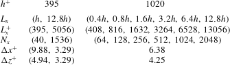
Reference Abe, Kawamura, Toh, Itano, Palma and Lopes2007). The domain size, number of grid points and spatial resolutions are listed in table 2. The smallest streamwise domain for
 $h^{+}=395$
and 1020 is
 $L_{x}^{+}\approx 400$
, which is the minimal unit of near-wall turbulence (Jiménez & Moin Reference Jiménez and Moin1991). We also compare our results with other DNS data obtained with different domain sizes (Lozano-Durán & Jiménez Reference Lozano-Durán and Jiménez2014; Lee & Moser Reference Lee and Moser2015).

4 Results for the energy dissipation function
$E$

4.1 Effect of the streamwise domain
We first clarify the effect of
 $L_{x}$
on the total energy dissipation
 $E$
. Distributions of
 $\langle {\it\nu}(\text{d}\bar{U}/\text{d}y)^{2}\rangle$
and
 $\langle \overline{{\it\varepsilon}}\rangle$
normalized by
 $U_{{\it\tau}}^{3}$
are shown in figure 1 as a function of
 $L_{x}/h$
for both
 $h^{+}=395$
and 1020. Also included in figure 1(a) are the data of Lozano-Durán & Jiménez (Reference Lozano-Durán and Jiménez2014) at
 $h^{+}=4179$
with
 $L_{x}=2{\rm\pi}h$
and Lee & Moser (Reference Lee and Moser2015) at
 $h^{+}=1000$
and 5186 with
 $L_{x}=8{\rm\pi}h$
since
 $\langle {\it\nu}(\text{d}\bar{U}/\text{d}y)^{2}\rangle /U_{{\it\tau}}^{3}$
is constant for
 $h^{+}\geqslant 300$
(see figure 3
a) and the departure from constancy corresponds to the
 $L_{x}$
effect. It is shown that the viscous energy dissipation rate
 $\langle {\it\nu}(\text{d}\bar{U}/\text{d}y)^{2}\rangle /U_{{\it\tau}}^{3}$
increases with decreasing
 $L_{x}$
when
 $L_{x}<2h$
. This is caused by the thickened buffer region as
 $L_{x}$
decreases (see figure 2
a where the distributions of
 $(\text{d}\bar{U}^{+}/\text{d}y^{+})^{2}$
are shown).
 $\langle \overline{{\it\varepsilon}}\rangle /U_{{\it\tau}}^{3}$
is however essentially unaffected by
 $L_{x}/h$
, whereas
 $\langle \overline{{\it\varepsilon}}_{11}\rangle /U_{{\it\tau}}^{3}$
(the streamwise component of the dissipation) is affected in a similar manner to
 $\langle {\it\nu}(\text{d}\bar{U}/\text{d}y)^{2}\rangle /U_{{\it\tau}}^{3}$
. This is closely associated with the energy redistribution where the pressure strain rate and pressure diffusion terms, viz.
 $$\begin{eqnarray}{\it\phi}_{ij}^{+}=\overline{p^{+}\left(\frac{\partial u_{i}^{+}}{\partial x_{j}^{+}}+\frac{\partial u_{j}^{+}}{\partial x_{i}^{+}}\right)}\end{eqnarray}$$
and
 $$\begin{eqnarray}{\it\varphi}_{ij}^{+}=-\!\left(\frac{\partial }{\partial x_{i}^{+}}\overline{u_{j}^{+}p^{+}}+\frac{\partial }{\partial x_{j}^{+}}\overline{u_{i}^{+}p^{+}}\right),\end{eqnarray}$$
Distributions of
 $\langle {\it\nu}(\text{d}\bar{U}/\text{d}y)^{2}\rangle /U_{{\it\tau}}^{3}$
and
 $\langle \overline{{\it\varepsilon}}\rangle /U_{{\it\tau}}^{3}$
in a channel flow as a function of
 $L_{x}/h$
: (a)
 $\langle {\it\nu}(\text{d}\bar{U}/\text{d}y)^{2}\rangle /U_{{\it\tau}}^{3}$
; (b)
 $\langle \overline{{\it\varepsilon}}\rangle /U_{{\it\tau}}^{3}$
.

Distributions of
 $(\text{d}\bar{U}^{+}/\text{d}y^{+})^{2}$
,
 ${\it\phi}_{ij}^{+}$
and
 ${\it\varphi}_{22}^{+}$
in a channel flow for
 $h^{+}=1020$
: (a)
 $(\text{d}\bar{U}^{+}/\text{d}y^{+})^{2}$
; (b)
 ${\it\phi}_{ij}^{+}$
and
 ${\it\varphi}_{22}^{+}$
.

play an important role. Distributions of
 ${\it\phi}_{ij}^{+}$
and
 ${\it\varphi}_{ij}^{+}$
are shown in figure 2(b) for
 $h^{+}=1020$
. The data of Lee & Moser (Reference Lee and Moser2015) for
 $h^{+}=1000$
with
 $L_{x}=8{\rm\pi}h$
are also plotted. For
 $L_{x}<6.4h$
, the magnitudes of
 ${\it\phi}_{11}^{+}$
,
 ${\it\phi}_{22}^{+}$
and
 ${\it\phi}_{33}^{+}$
are attenuated significantly due to the impaired global nature of the pressure, i.e. the turbulent kinetic energy is not redistributed properly to
 $\overline{v^{+}v^{+}}$
and
 $\overline{w^{+}w^{+}}$
. In particular, the rate of decrease in
 ${\it\phi}_{11}^{+}$
and
 ${\it\phi}_{33}^{+}$
with decreasing
 $L_{x}/h$
is large, which makes
 $\overline{u^{+}u^{+}}$
and
 $\overline{w^{+}w^{+}}$
more and less energetic, respectively. This result implies that the inactive motion is affected more significantly by
 $L_{x}$
than the active motion. Note that the inactive motion refers to the large-scale motion (or structure) and the irrotational pressure fluctuations of the outer region (Townsend Reference Townsend1961; Bradshaw Reference Bradshaw1967) which contribute to the Reynolds normal stress (mostly to the low-wavenumber components of
 $\overline{u^{+}u^{+}}$
and
 $\overline{w^{+}w^{+}}$
as described by Townsend’s (Reference Townsend1976) attached eddy model) in the inner region, while the active motion contributes almost exclusively to the Reynolds shear stress (see also § 6 of Antonia et al. (Reference Antonia, Teitel, Kim and Browne1992)) in this region.
 $\overline{{\it\varepsilon}}_{11}$
(the streamwise component of the dissipation) and
 $\overline{{\it\varepsilon}}_{33}$
(the spanwise component of the dissipation) become therefore larger and smaller with decreasing
 $L_{x}/h$
. This leads to an increase in
 $\langle \overline{{\it\varepsilon}}_{11}\rangle /U_{{\it\tau}}^{3}$
and decrease in
 $\langle \overline{{\it\varepsilon}}_{33}\rangle /U_{{\it\tau}}^{3}$
(figure 1
b), and hence a small dependence on
 $L_{x}/h$
of
 $\langle \overline{{\it\varepsilon}}\rangle /U_{{\it\tau}}^{3}$
since the sum of
 $\langle \overline{{\it\varepsilon}}_{11}\rangle /U_{{\it\tau}}^{3}$
,
 $\langle \overline{{\it\varepsilon}}_{22}\rangle /U_{{\it\tau}}^{3}$
,
 $\langle \overline{{\it\varepsilon}}_{33}\rangle /U_{{\it\tau}}^{3}$
is equal to
 $2\langle \overline{{\it\varepsilon}}\rangle /U_{{\it\tau}}^{3}$
. This is the reason why the
 $L_{x}$
effect does not appear in
 $\langle \overline{{\it\varepsilon}}\rangle /U_{{\it\tau}}^{3}$
explicitly. The present criterion of
 $L_{x}=6.4h$
is identical with the finding of Lozano-Durán & Jiménez (Reference Lozano-Durán and Jiménez2014) that correct one-point statistics are obtained when
 $L_{x}$
is larger than
 $2{\rm\pi}h$
. This criterion is most likely associated with the streamwise extent of the large-scale structures (Balakumar & Adrian (Reference Balakumar and Adrian2007) reported 2–
 $3{\it\delta}$
), but not very large-scale structures (Monty et al. (Reference Monty, Stewart, Williams and Chong2007) reported long meandering features up to
 $25{\it\delta}$
long in the channel and pipe) since the latter are very long structures and exhibit a shallow angle to the wall so that they may be thought of as the wall-parallel mode (i.e. the zero mode in the energy spectra). The required
 $L_{x}$
in the DNS is obviously shorter than that in the experiment since the DNS is started with the fully developed turbulent state. In the DNS, once the velocity field reaches the statistically steady state (viz. a linear profile of the total shear stress), the Navier–Stokes equations are integrated further in time to obtain various turbulence statistics.
Distributions of
 $\langle {\it\nu}(\text{d}\bar{U}/\text{d}y)^{2}\rangle /U_{{\it\tau}}^{3}$
and
 $\langle \overline{{\it\varepsilon}}\rangle /U_{{\it\tau}}^{3}$
in a channel flow as a function of
 $h^{+}$
: (a)
 $\langle {\it\nu}(\text{d}\bar{U}/\text{d}y)^{2}\rangle /U_{{\it\tau}}^{3}$
; (b)
 $\langle \overline{{\it\varepsilon}}\rangle /U_{{\it\tau}}^{3}$
.

4.2 Reynolds number dependence
We now quantify the
 $h^{+}$
dependence of the total energy dissipation rate by considering the DNS data in which
 $L_{x}\geqslant 2{\rm\pi}h$
. The normalized values of
 $\langle \overline{{\it\varepsilon}}\rangle$
and
 $\langle {\it\nu}(\text{d}\bar{U}/\text{d}y)^{2}\rangle$
are plotted in figure 3 (on linear–log scales) in terms of
 $h^{+}$
using the present and existing DNS data. The viscous energy dissipation rate
 $\langle {\it\nu}(\text{d}\bar{U}/\text{d}y)^{2}\rangle /U_{{\it\tau}}^{3}$
(figure 3
a) is essentially constant for
 $h^{+}\geqslant 300$
; the value of the constant (
 $=$
9.13) is the same as that reported by Laadhari (Reference Laadhari2007), who noted that this constancy applies for
 $h^{+}\geqslant 500$
, when
 $\langle \overline{{\it\varepsilon}}\rangle /U_{{\it\tau}}^{3}$
exceeds
 $\langle {\it\nu}(\text{d}\bar{U}/\text{d}y)^{2}\rangle /U_{{\it\tau}}^{3}$
. The value of
 $\langle {\it\nu}(\text{d}\bar{U}/\text{d}y)^{2}\rangle /U_{{\it\tau}}^{3}$
seems to be identical with the values obtained in either a pipe or a boundary layer (see figure 3
a where the data of Wu & Moin (Reference Wu and Moin2008) in a pipe flow and Schlatter & Örlü (Reference Schlatter and Örlü2010) in a zero-pressure-gradient boundary layer are included in terms of
 $R^{+}$
(
 $R$
is the pipe radius) and
 ${\it\delta}_{99}^{+}$
(
 ${\it\delta}_{99}$
is the 99 % boundary layer thickness), respectively). This is consistent with the good collapse in the near-wall distribution of
 $\bar{U}^{+}$
in terms of
 $y^{+}$
for these three flows; the inner layer similarity of
 $\bar{U}^{+}$
leads to the constancy of
 $\langle {\it\nu}(\text{d}\bar{U}/\text{d}y)^{2}\rangle /U_{{\it\tau}}^{3}$
. Klebanoff (Reference Klebanoff1954) also noted that the viscous energy dissipation rate is negligible above
 $y^{+}\approx 30$
for the three flows (see also figure 2
a where the distribution of
 $(\text{d}\bar{U}^{+}/\text{d}y^{+})^{2}$
is shown at
 $h^{+}=1020$
). On the other hand,
 $\langle \overline{{\it\varepsilon}}\rangle /U_{{\it\tau}}^{3}$
(figure 3
b) increases logarithmically with increasing
 $h^{+}$
over the same range of
 $h^{+}$
(viz.
 $h^{+}\geqslant 300$
). This increase is well described by
 $$\begin{eqnarray}\langle \overline{{\it\varepsilon}}\rangle /U_{{\it\tau}}^{3}=2.54\ln (h^{+})-6.72,\end{eqnarray}$$
which is obtained by substituting the relation for
 $U_{b}^{+}$
(4.6) and the constant value (
 $=$
9.13) for
 $\langle {\it\nu}(\text{d}\bar{U}/\text{d}y)^{2}\rangle /U_{{\it\tau}}^{3}$
into (2.7). Viscosity affects
 $\langle \overline{{\it\varepsilon}}\rangle$
and
 $\langle {\it\nu}(\text{d}\bar{U}/\text{d}y)^{2}\rangle$
significantly below
 $h^{+}=300$
since there is no clear separation between the inner and outer regions.
To ensure the accuracy of
 $\langle \overline{{\it\varepsilon}}\rangle$
and
 $\langle {\it\nu}(\text{d}\bar{U}/\text{d}y)^{2}\rangle$
, the ratios
 $$\begin{eqnarray}{\it\xi}=\langle P_{k}\rangle /\langle \overline{{\it\varepsilon}}\rangle\end{eqnarray}$$
and
 $$\begin{eqnarray}{\it\psi}=(\langle \overline{{\it\varepsilon}}\rangle +\langle {\it\nu}(\text{d}\bar{U}/\text{d}y)^{2}\rangle )/U_{{\it\tau}}^{2}U_{b}\end{eqnarray}$$
should be equal to 1 (see also (2.6) and (2.7)). Several DNS data, including the present data, indicate that the departure from 1 of the ratios
 ${\it\xi}$
and
 ${\it\psi}$
is almost negligible (figure 4), thus confirming the accuracy of these simulations. From a historical perspective, it is of interest to note that the earliest attempt to test
 $\overline{{\it\varepsilon}_{iso\,2}}$
, measured in a turbulent channel flow, was made in Taylor’s (Reference Taylor1935) seminal paper where the isotropic expressions
 $\overline{{\it\varepsilon}_{iso}}=15{\it\nu}\overline{(\partial u/\partial x)^{2}}$
and
 $\overline{{\it\varepsilon}_{iso\,2}}=7.5{\it\nu}\overline{(\partial u/\partial y)^{2}}$
were first derived. In essence, Taylor (Reference Taylor1935) was testing (2.6), except that his integration was started at the centre of the channel and the upper limit of the integration did not quite go to the wall (the measurement location closest to the wall was
 $y/h\approx 0.08$
). By extrapolating the data to the wall, we estimate that
 $\langle P_{k}\rangle /\langle \overline{{\it\varepsilon}_{iso2}}\rangle$
could be somewhat greater than 2. This is, perhaps surprisingly, not an implausible outcome since the contribution from
 $\langle {\it\nu}(\text{d}\bar{U}/\text{d}y)^{2}\rangle$
is likely to be comparable to that of
 $\langle \overline{{\it\varepsilon}}\rangle$
at this Reynolds number (
 $h^{+}\approx 450$
),
 $\langle \overline{{\it\varepsilon}_{iso\,2}}\rangle$
is likely to overestimate
 $\langle \overline{{\it\varepsilon}}\rangle$
(inset of figure 4
a) and the aspect ratio of the channel was only 4. In experiments, data for
 $\langle \overline{{\it\varepsilon}}\rangle /U_{{\it\tau}}^{3}$
and
 $\langle {\it\nu}(\text{d}\bar{U}/\text{d}y)^{2}\rangle /U_{{\it\tau}}^{3}$
are not usually available. A possible formula for
 $U_{b}^{+}$
can however be established from the experimental data.
Distributions of
 ${\it\xi}$
and
 ${\it\psi}$
in a channel flow as a function of
 $h^{+}$
: (a)
 ${\it\xi}$
; (b)
 ${\it\psi}$
.

Distributions of
 $U_{b}^{+}$
in a channel flow for all available DNS data and several sets of experimental data are shown in figures 5(a) and (b), respectively. A least squares fit to the DNS data in figure 5(a) over the range
 $h^{+}\geqslant 300$
yields
 $$\begin{eqnarray}U_{b}^{+}(\equiv U_{b}/U_{{\it\tau}})=2.54\ln (h^{+})+2.41,\end{eqnarray}$$
or, equivalently,
 $$\begin{eqnarray}\frac{1}{\sqrt{C_{f}}}=1.80\ln \left(Re_{b}\sqrt{C_{f}}\right)-0.163.\end{eqnarray}$$
This relation represents a good fit to nearly all the experimental data for
 $U_{b}^{+}$
over more than one decade of
 $h^{+}$
(see figure 5
b). Also included in figure 5 are relations for
 $U_{b}^{+}$
, originally established for the skin friction coefficient
 $C_{f}$
by Dean (Reference Dean1978) and Zanoun et al. (Reference Zanoun, Nagib and Durst2009), which can be written as
 $$\begin{eqnarray}U_{b}^{+}=7.32\,h^{+1/7}\end{eqnarray}$$
and
 $$\begin{eqnarray}U_{b}^{+}=2.702\ln (h^{+})+0.997,\end{eqnarray}$$
respectively. Dean’s (Reference Dean1978) relation (4.8) appears to represent the data adequately over almost the complete range of
 $h^{+}$
. However, the concave curvature exhibited by (4.8) is not discernible in the overall trend of the data and implies that the difference between the logarithmic dependence (4.6) and the power-law relation (4.8) will become more perceptible as
 $h^{+}$
extends beyond
 $10^{4}$
.
Distributions of
 $U_{b}^{+}$
in a channel flow as a function of
 $h^{+}$
: (a) DNS; (b) experiment.

Note that among the experimental data included in figure 5(b),
 $U_{{\it\tau}}$
was most likely underestimated by Comte-Bellot (Reference Comte-Bellot1963) (
 $AR=13.3$
,
 $L=133h$
) (see also Abe & Antonia Reference Abe and Antonia2011). For the latter data, correction was hence made for
 $U_{{\it\tau}}$
using (4.7); the resulting values of
 $U_{b}^{+}$
lie much closer to relation (4.6) than the original values (see figure 5
b). For more recent experiments, special care was taken in determining
 $U_{{\it\tau}}$
. Zanoun et al. (Reference Zanoun, Durst and Nagib2003) (also Zanoun et al.
Reference Zanoun, Nagib and Durst2009) obtained close agreement between
 ${\it\tau}_{w}$
determined from the static pressure distribution along the fully developed part of the channel (aspect ratio
 $AR=12$
and length
 $L=260h$
) and that estimated using oil film interferometry. Their hot-wire data covered the range
 $1167<h^{+}<4783$
. Fischer, Jovanović & Durst (Reference Fischer, Jovanović and Durst2001) determined
 $U_{{\it\tau}}$
from a polynomial fit to the mean velocity in the viscous sublayer and the lower part of the buffer region. Their LDA measurements in a water channel (
 $AR=18$
,
 $L=200h$
), acquired with good spatial and temporal resolution, extended up to
 $h^{+}\approx 480$
. Earlier, Durst et al. (Reference Durst, Fischer, Jovanović and Kimura1998) reported results in the same channel over the range
 $87<h^{+}<293$
. Shah (Reference Shah1988) (
 $AR=18.1$
,
 $L=349h$
) and Hussain & Reynolds (Reference Hussain and Reynolds1975) (
 $AR=16.4$
,
 $L=460h$
) conducted measurements with long channels for
 $h^{+}=187{-}1357$
and 637–1383, respectively, to ensure
 $\text{d}\bar{P}/\text{d}x=\text{const.}$
and hence accuracy of
 $U_{{\it\tau}}$
. Bakken et al. (Reference Bakken, Krogstad, Ashrafian and Andersson2005) made measurements in both smooth and rough walls (
 $AR=14$
,
 $L=100h$
). In their smooth wall case,
 $h^{+}$
ranges from 360 to 3300;
 $U_{{\it\tau}}$
was determined from both the mean pressure gradient and the Reynolds shear stress using the total shear stress relation. Monty (Reference Monty2005) obtained
 $U_{{\it\tau}}$
using the mean pressure gradient in a channel (
 $AR=11.7$
,
 $L=205h$
) for
 $h^{+}\approx 380{-}4000$
. Monty’s data for
 $U_{b}^{+}$
are in reasonable agreement with those of Zanoun et al. (Reference Zanoun, Durst and Nagib2003) (also Zanoun et al.
Reference Zanoun, Nagib and Durst2009) when
 $h^{+}$
exceeds approximately 2000. Schultz & Flack (Reference Schultz and Flack2013) also obtained
 $U_{{\it\tau}}$
using (1.1) in their LDV measurements (
 $AR=8$
,
 $L=248h$
) for
 $h^{+}=1010{-}5900$
. These experimental data indeed provide strong support for relation (4.6) in figure 5(b). The logarithmic variation of
 $U_{b}^{+}$
, established from DNS data up to
 $h^{+}=5000$
, can be extrapolated to values of
 $h^{+}$
that extend to approximately
 $10^{4}$
.
It should also be noted that the logarithmic relation (4.6) is a better fit to both the DNS and experimental data than (4.9) for
 $h^{+}<2000$
, possibly because the present
 $U_{b}^{+}$
relation (4.6) is based on (2.7), whereas Zanoun et al. (Reference Zanoun, Nagib and Durst2009) obtained the
 $U_{b}^{+}$
relation (4.9) from the velocity log law (1.4). This difference cannot be dismissed given that, unlike the velocity log law, the skin friction law (4.6) is established unambiguously for
 $h^{+}>300$
.
4.3 Extension to a pipe flow
Given that the sum of the integrals of the mean and turbulent energy dissipation rates is equal to the non-dimensional energy input from the mean pressure gradient
 $(U_{b}^{+})$
in internal flows (i.e. (2.7)) and that as in a channel (i.e. (4.3)),
 $\langle \overline{{\it\varepsilon}}\rangle /U_{{\it\tau}}^{3}$
exhibits the
 $2.54\ln (R^{+})$
dependence in a pipe (see § 4.5), it would be straightforward to check if the slope of
 $U_{b}^{+}$
(viz.
 $\ln (h^{+})$
versus
 $h^{+}$
) obtained in the channel (viz. the slope of (4.6)) also applies to the pipe. In the latter flow, Prandtl (see Schlichting Reference Schlichting1979) established the well-known law for the friction factor
 ${\it\lambda}(=4C_{f})$
based on Nikuradse’s (Reference Nikuradse1932) data, viz.
 $$\begin{eqnarray}1/\sqrt{{\it\lambda}}=2.0\log \left(Re_{b}\sqrt{{\it\lambda}}\right)-0.8.\end{eqnarray}$$
This equation can be rewritten as
 $$\begin{eqnarray}U_{b}^{+}=2.46\ln (R^{+})+2.0.\end{eqnarray}$$
The present relation, based on the Reynolds number dependence of
 $\langle \overline{{\it\varepsilon}}\rangle /U_{{\it\tau}}^{3}$
, is written as
 $$\begin{eqnarray}U_{b}^{+}=2.54\ln (R^{+})+1.31,\end{eqnarray}$$
which is close to Prandtl’s relation. Clearly, (4.12) gives a reasonable fit to the DNS and experimental data in the range
 $R^{+}=300{-}10^{4}$
(see figure 6). The magnitude of
 $U_{b}^{+}$
is approximately 5 % larger in the channel than in the pipe. On the other hand, while there is reasonable inner layer similarity in the distributions of
 $\bar{U}^{+}$
, the magnitude of
 $\bar{U}^{+}$
is larger in the pipe than in the channel in the outer region (see Monty et al.
Reference Monty, Hutchins, Ng, Marusic and Chong2009; see also figure 12 where
 $\overline{{\it\varepsilon}}{\it\delta}/U_{{\it\tau}}^{3}$
(
 ${\it\delta}$
denotes either
 $h$
,
 $R$
or
 ${\it\delta}_{99}$
) shows the same trend as
 $\bar{U}^{+}$
). The difference in
 $U_{b}^{+}$
is thus most likely due to a difference in geometry between these two flows.
Distributions of
 $U_{b}^{+}$
in a pipe flow as a function of
 $R^{+}$
.

It is worthwhile mentioning that the present skin friction relation for the pipe (4.12) is quite close to that obtained by Furuichi et al. (Reference Furuichi, Terao, Wada and Tsuji2015) using LDV measurements in the range
 $4\times 10^{2}<R^{+}<2.7\times 10^{5}$
, viz.
 $$\begin{eqnarray}1/\sqrt{{\it\lambda}}=2.090\log \left(Re_{b}\sqrt{{\it\lambda}}\right)-1.172.\end{eqnarray}$$
The corresponding expression for
 $U_{b}^{+}$
is
 $$\begin{eqnarray}U_{b}^{+}=2.57\ln (R^{+})+1.13.\end{eqnarray}$$
Both (4.12) and (4.14) give a reasonable fit to the data for lower Reynolds numbers than those at which the velocity log law is established.
Distributions of
 $\overline{U}$
and
 $\overline{{\it\varepsilon}}$
with the inner and outer scalings: (a)
 $\overline{U}^{+}$
; (b)
 $\overline{{\it\varepsilon}}{\it\nu}/U_{{\it\tau}}^{4}$
; (c)
 $(U_{0}-\overline{U})/U_{{\it\tau}}$
; (d)
 $\overline{{\it\varepsilon}}h/U_{{\it\tau}}^{3}$
. Note that
 $U_{0}$
denotes the centreline mean velocity.

4.4 Scaling laws of
$\overline{{\it\varepsilon}}$
and matching argument

Here, we focus on the scaling of
 $\overline{{\it\varepsilon}}$
in different regions of the channel. There have been a number of observations indicating that the classical inner scaling,
 $$\begin{eqnarray}\overline{{\it\varepsilon}}^{+}\equiv \overline{{\it\varepsilon}}{\it\nu}/U_{{\it\tau}}^{4}=f(y^{+}),\end{eqnarray}$$
does not hold, the normalized distributions of
 $\overline{{\it\varepsilon}}^{+}$
in the wall region exhibiting a non-negligible dependence on
 $h^{+}$
(Antonia, Kim & Browne Reference Antonia, Kim and Browne1991; Hoyas & Jiménez Reference Hoyas and Jiménez2008). On the other hand, there is adequate evidence that the outer scaling,
 $$\begin{eqnarray}\overline{{\it\varepsilon}}h/U_{{\it\tau}}^{3}=g(y/h),\end{eqnarray}$$
is satisfied closely in the outer region of the channel (see Hoyas & Jiménez Reference Hoyas and Jiménez2008; Abe & Antonia Reference Abe and Antonia2011). Distributions of
 $\overline{{\it\varepsilon}}$
with inner and outer scalings are shown in figure 7 together with those of
 $\overline{U}$
. The magnitude of
 $\overline{{\it\varepsilon}}^{+}$
increases with
 $h^{+}$
close to the wall due to the effect of the inactive motion (see Hoyas & Jiménez Reference Hoyas and Jiménez2008), while
 $\overline{{\it\varepsilon}}^{+}$
seems to collapse for
 $y^{+}\geqslant 20$
provided
 $h^{+}\geqslant 300$
(figure 7
b). In contrast to the mean velocity, viscous effects are unlikely to affect the energy dissipation rate significantly for
 $y^{+}>20$
. This is associated with Bradshaw’s (Reference Bradshaw1967) observation that the only noticeable effect of the inactive motion is an increased dissipation of kinetic energy into heat in the viscous sublayer. For
 $y^{+}>20$
,
 $-\overline{uv}=\text{const.}$
is also satisfied reasonably well when
 $h^{+}$
is large enough (see figure 10
b). On the other hand, unlike
 $\overline{U}$
,
 $\overline{{\it\varepsilon}}$
collapses almost perfectly on
 $U_{{\it\tau}}^{3}$
and
 $h$
in the region
 $20/h^{+}<y/h<1$
(figure 7
d; see also figure 9
b where the location
 $20/h^{+}$
is identified by the dashed vertical lines). In this context, McKeon & Morrison (Reference McKeon and Morrison2007) indicated that the similarity in
 $\overline{{\it\varepsilon}}$
is obtained for
 $R^{+}>5000$
in a pipe by analysing the superpipe data, in which estimates for
 $\overline{{\it\varepsilon}}$
are made by invoking
 $P_{k}=\overline{{\it\varepsilon}}$
. The present results indicate that the outer layer similarity for
 $\overline{{\it\varepsilon}}$
is more convincing than that for
 $\overline{U}$
even at small
 $h^{+}$
(
 $h^{+}\geqslant 300$
) (see figure 7
c,d).
We now apply a matching argument to
 $\overline{{\it\varepsilon}}$
. Here, we assume that
 $h^{+}$
is large enough to have a clear distinction between inner and outer regions, and that there is a region where relations (4.15) and (4.16) overlap so that the gradient of
 $\overline{{\it\varepsilon}}$
should coincide, viz.
 $$\begin{eqnarray}\frac{\text{d}\overline{{\it\varepsilon}}}{\text{d}y}=\frac{U_{{\it\tau}}^{5}}{{\it\nu}^{2}}\frac{\text{d}f}{\text{d}y^{+}}=\frac{U_{{\it\tau}}^{3}}{h^{2}}\frac{\text{d}g}{\text{d}y^{\ast }},\end{eqnarray}$$
where
 $y^{\ast }\equiv y/h$
. After multiplying by
 $y^{2}$
, the equality between the second and third members of (4.17) becomes
 $$\begin{eqnarray}y^{+^{2}}\frac{\text{d}f}{\text{d}y^{+}}=y^{\ast ^{2}}\frac{\text{d}g}{\text{d}y^{\ast }}.\end{eqnarray}$$
This is satisfied if
 $$\begin{eqnarray}\frac{\text{d}f}{\text{d}y^{+}}=\frac{D}{y^{+^{2}}}\quad \text{or}\quad \frac{\text{d}g}{\text{d}y^{\ast }}=\frac{D}{y^{\ast ^{2}}}.\end{eqnarray}$$
Equation (4.18) indicates that
 $\overline{{\it\varepsilon}}$
should indeed scale with
 $U_{{\it\tau}}^{3}$
and
 $y$
in the overlap region. After integrating (4.19a,b
), we obtain
 $$\begin{eqnarray}f=-\frac{D}{y^{+}}+D_{1}\quad \text{or}\quad g=-\frac{D}{y^{\ast }}+D_{2}.\end{eqnarray}$$
Here, we adopt a small parameter
 ${\it\gamma}=1/h^{+}$
and an outer variable
 $y^{\ast }={\it\gamma}y^{+}$
as was done by Afzal (Reference Afzal1976) for the mean velocity gradient and obtain
 $D_{1}=-{\it\gamma}c$
and
 $D_{2}=-c$
. Equation (4.20a,b
) is then rewritten as
 $$\begin{eqnarray}f=-\frac{D}{y^{+}}-{\it\gamma}c\quad \text{or}\quad {\it\gamma}g=-{\it\gamma}\frac{D}{y^{\ast }}-{\it\gamma}c,\end{eqnarray}$$
where
 $c$
is a constant. After the normalization, it follows from (4.21a,b
) that the overlap scaling may be written as
 $$\begin{eqnarray}\overline{{\it\varepsilon}}y/U_{{\it\tau}}^{3}=1/{\it\kappa}_{{\it\varepsilon}}-c(y^{+}/h^{+})\end{eqnarray}$$
and
 $$\begin{eqnarray}\overline{{\it\varepsilon}}y/U_{{\it\tau}}^{3}=1/{\it\kappa}_{{\it\varepsilon}}-c(y/h)\end{eqnarray}$$
in inner and outer coordinates, respectively, where
 $D=-1/{\it\kappa}_{{\it\varepsilon}}$
and
 ${\it\kappa}_{{\it\varepsilon}}$
is a constant. The matching argument highlights that the overlap scaling of
 $\overline{{\it\varepsilon}}$
requires neither the existence of a velocity log law nor energy equilibrium
 $(P_{k}=\overline{{\it\varepsilon}})$
. It does however require the Reynolds number to be large enough (
 $h^{+}\approx 300$
) to allow the overlap region, where the relevant length scale is the distance from the wall,
 $y$
to be distinguished unambiguously. In the overlap region, when
 $-\overline{uv}\simeq \text{const.}$
(this constancy is plausible only when
 $h^{+}$
is large enough) (see figure 10
b),
 $P_{k}y/U_{{\it\tau}}^{3}\approx y\text{d}\bar{U}^{+}/\text{d}y$
(see figures 10
c and 11
a) and
 $P_{k}/\overline{{\it\varepsilon}}\approx 1$
(see figure 10
a). Equations (4.22) and (4.23) are analogous to the generalized velocity log law for the channel flow proposed by Jiménez & Moser (Reference Jiménez and Moser2007) using the asymptotic matching of the mean velocity gradient,
 $$\begin{eqnarray}y\frac{\text{d}\bar{U}^{+}}{\text{d}y}=\frac{1}{{\it\kappa}}+{\it\alpha}\frac{y^{+}}{h^{+}}+\frac{{\it\beta}}{h^{+}}\end{eqnarray}$$
and
 $$\begin{eqnarray}y\frac{\text{d}\bar{U}^{+}}{\text{d}y}=\frac{1}{{\it\kappa}}+{\it\alpha}\frac{y}{h}+\frac{{\it\beta}}{h^{+}}\end{eqnarray}$$
in inner and outer coordinates, respectively, with
 $1/{\it\kappa}=2.49$
,
 ${\it\alpha}=1.0$
and
 ${\it\beta}=150$
. While both the present study and that of Jiménez & Moser (Reference Jiménez and Moser2007) use a matching argument, there are discernible differences between (4.22) and (4.23) and (4.24) and (4.25) in terms of the constants (i.e.
 ${\it\kappa}_{{\it\varepsilon}}$
and
 ${\it\kappa}$
) and in the limits of applicability of the overlap expressions (i.e.
 $30/h^{+}\leqslant y/h\leqslant 0.2$
in (4.22) and (4.23) (this is discussed below) and
 $300/h^{+}<y/h<0.45$
in (4.24) and (4.25)).
Distributions of
 $\overline{{\it\varepsilon}}y/U_{{\it\tau}}^{3}$
in a channel, pipe and boundary layer: (a) channel (in terms of
 $y^{+}$
); (b) boundary layer (in terms of
 $y^{+}$
); (c) channel (in terms of
 $y/h$
); (d) pipe (in terms of
 $y/R$
). In (c), line patterns are the same as in (a).

In (4.22) and (4.23), the second terms on the right-hand sides are responsible for the finite Reynolds number effect, i.e.
 $-c(y^{+}/h^{+})$
(the second term of (4.22)) goes to zero as
 $h^{+}\rightarrow \infty$
, while
 $-c(y/h)$
(the second term of (4.23)) does not depend on
 $h^{+}$
but may enhance the outer limit of the overlap scaling. When the finite Reynolds number effect disappears, equations (4.22) and (4.23) reduce to
 $\overline{{\it\varepsilon}}y/U_{{\it\tau}}^{3}=1/{\it\kappa}_{{\it\varepsilon}}$
analogous to the classical scaling based on the velocity log law
 $\overline{{\it\varepsilon}}y/U_{{\it\tau}}^{3}=1/{\it\kappa}$
(see, for example, Townsend Reference Townsend1976). Note that
 ${\it\kappa}_{{\it\varepsilon}}$
is identical with
 ${\it\kappa}$
only if the velocity log law and energy equilibrium conditions are satisfied. Hoyas & Jiménez (Reference Hoyas and Jiménez2008) found that the magnitudes of all the terms in the budgets of
 $\overline{u_{i}u_{j}}$
and
 $k$
in the channel decrease almost proportionally to
 $y^{-1}$
in the region
 $y^{+}=50$
to
 $y/h=0.4$
for
 $h^{+}=2003$
. Figure 8(a) highlights that the largest magnitude of
 $\overline{{\it\varepsilon}}y/U_{{\it\tau}}^{3}$
(
 $=$
2.54) is attained at
 $y^{+}=30{-}40$
. This value is the same for the channel, pipe and boundary layer due to the wall similarity of the constant stress region (Townsend Reference Townsend1976). It depends on the Reynolds number in the channel and pipe, but not in the boundary layer (see figure 8). This finite Reynolds number effect comes from the
 $\text{d}\overline{P}/\text{d}x$
effect, which reduces the magnitude of
 $-\overline{uv}$
and hence
 $P_{k}$
and
 $\overline{{\it\varepsilon}}$
when
 $h^{+}$
is small. On the other hand, this effect is negligible when
 $h^{+}\approx 5000$
, which allows us to determine
 $1/{\it\kappa}_{{\it\varepsilon}}$
unambiguously. Indeed,
 $1/{\it\kappa}_{{\it\varepsilon}}=2.54$
is identified asymptotically for
 $h^{+}\geqslant 5000$
in the channel (figure 8
a), while this value is obtained for
 ${\it\delta}_{99}^{+}\geqslant 300$
in the zero-pressure-gradient boundary layer due to the absence of the
 $\text{d}\overline{P}/\text{d}x$
effect (figure 8
b). A fit to the DNS data over
 $30/{\it\delta}^{+}\leqslant y/{\it\delta}\leqslant 0.2$
then yields
 $c=2.6$
, 1.3 and 0 in the channel, pipe and boundary layer. Indeed, equations (4.22) and (4.23) reproduce the
 $h^{+}$
dependence of the peak magnitude of
 $\overline{{\it\varepsilon}}y/U_{{\it\tau}}^{3}$
successfully for
 $h^{+}\geqslant 300$
and provide a good fit to the data in the region
 $30/h^{+}\leqslant y/h\leqslant 0.2$
(see figure 8
c). While the classical overlap argument based on
 $\bar{U}$
(Millikan Reference Millikan1938) strictly holds only at large
 $h^{+}$
, the overlap region for
 $\overline{{\it\varepsilon}}$
is established at small
 $h^{+}$
(
 ${\approx}$
300) (see also figure 8
c in which the DNS data for
 $h^{+}=395$
follow the present overlap scaling very well).
Distributions of
 $\overline{{\it\varepsilon}}{\it\nu}/U_{{\it\tau}}^{4}$
and
 $\overline{{\it\varepsilon}}h/U_{{\it\tau}}^{3}$
in a channel flow with log–log coordinates: (a)
 $\overline{{\it\varepsilon}}{\it\nu}/U_{{\it\tau}}^{4}$
; (b)
 $\overline{{\it\varepsilon}}h/U_{{\it\tau}}^{3}$
. – ⋅ – ⋅ –,
 $h^{+}=180$
;
 $\cdots \cdots$
,
 $h^{+}=395$
; – – – –,
 $h^{+}=640$
; ——,
 $h^{+}=1020$
; - ⋅ - ⋅ - ⋅ -,
 $h^{+}=1440$
(Hu et al.
Reference Hu, Morfey and Sandham2006); — ⋅ ⋅ — ⋅ ⋅ —,
 $h^{+}=2003$
(Hoyas & Jiménez Reference Hoyas and Jiménez2008); — —,
 $h^{+}=4079$
(Bernardini et al.
Reference Bernardini, Pirozzoli and Orlandi2014); - - - - - -,
 $h^{+}=5186$
(Lee & Moser Reference Lee and Moser2015);


Distributions of
 $P_{k}/\overline{{\it\varepsilon}}$
,
 $-\overline{u^{+}v^{+}}$
,
 ${\it\tau}^{+}$
and
 $y^{+}(\text{d}\bar{U}^{+}/\text{d}y^{+})$
in a channel flow: (a)
 $P_{k}/\overline{{\it\varepsilon}}$
; (b)
 $-\overline{u^{+}v^{+}}$
and
 ${\it\tau}^{+}$
; (c)
 $y^{+}(\text{d}\bar{U}^{+}/\text{d}y^{+})$
. In (b), line patterns are the same as in (a).

In the outer region (
 $y/h>0.2$
), there is still a decrease in
 $\overline{{\it\varepsilon}}y/U_{{\it\tau}}^{3}$
towards the centreline (see figure 11
b). After the fit to the DNS data in figure 7(d), the decrease is approximated closely by the outer scaling, viz.
 $$\begin{eqnarray}\overline{{\it\varepsilon}}h/U_{{\it\tau}}^{3}=2.45/(y/h)-d,\end{eqnarray}$$
with
 $d=1.7$
. Figure 9(b) underlines that (4.26) is a good fit in the region
 $20/h^{+}<y/h<1$
(see the thick lines in figure 9
b). Equation (4.26) also applies to the pipe reasonably well albeit with a different value of
 $d$
. In the boundary layer, it applies only below
 $y/{\it\delta}_{99}\approx 0.4$
, with yet another value of
 $d$
(see figure 12 where
 $d=0.9$
and
 $-1.0$
for the pipe and boundary layer, respectively). The different magnitudes of
 $d$
are most likely associated with the different flow characteristics (e.g. effects of the mean pressure gradient in the channel and pipe, curvature in the pipe and the presence of the turbulent/non-turbulent interface in the boundary layer). The present results underline that, as for the mean velocity, there is a discernible departure from similarity in the energy dissipation rate for the channel, pipe and boundary layer.
The excellent agreement with (4.26) in both the channel and pipe is due to the
 $\text{d}\bar{P}/\text{d}x$
effect. This latter effect seems to be responsible for yielding nearly the same slope (i.e. 2.45) as in the overlap scaling (i.e.
 $1/{\it\kappa}_{{\it\varepsilon}}=2.54$
) so that a reasonable collapse on the outer scaling is obtained over a wider range
 $20/h^{+}<y/h<1$
(see figure 9
b) than for the velocity log law, usually between
 $y^{+}\simeq 30$
and
 $y/h=0.2$
. A nearly identical observation was made for
 $\bar{U}$
by Monty et al. (Reference Monty, Stewart, Williams and Chong2007) who noted that the pipe and channel mean velocity profiles lie closer to the log law than in the boundary layer beyond
 $y/{\it\delta}=0.15$
. In the region
 $20<y^{+}<h^{+}$
, there is satisfactory collapse on inner scaling with the same slope (i.e. 2.45) as for outer scaling, viz.
 $$\begin{eqnarray}\overline{{\it\varepsilon}}{\it\nu}/U_{{\it\tau}}^{4}=2.45/y^{+}-d/h^{+}\end{eqnarray}$$
(see figure 9
a). Note that since it seems difficult to make a clear distinction between the overlap and outer regions of
 $\overline{{\it\varepsilon}}$
in the channel (see figure 9 where the inner and outer scalings (4.26), (4.27) hold reasonably well in the region
 $20/h^{+}<y/h<1$
), we assume that the upper bound of the overlap region of
 $\overline{{\it\varepsilon}}$
is
 $y/h=0.2$
, as is normally assumed for the velocity log law. In the present work, the overlap region of
 $\overline{{\it\varepsilon}}$
is thus defined by the region
 $30/h^{+}\leqslant y/{\it\delta}\leqslant 0.2$
, in which (4.22) and (4.23) hold quite well.
Distributions of
 $P_{k}y/U_{{\it\tau}}^{3}$
and
 $\overline{{\it\varepsilon}}y/U_{{\it\tau}}^{3}$
in a channel, pipe and boundary layer at
 ${\it\delta}^{+}\approx 1000$
: (a)
 $P_{k}y/U_{{\it\tau}}^{3}$
; (b)
 $\overline{{\it\varepsilon}}y/U_{{\it\tau}}^{3}$
.

Distributions of
 $\overline{{\it\varepsilon}}{\it\delta}/U_{{\it\tau}}^{3}$
in a channel, pipe and boundary layer at
 ${\it\delta}^{+}\approx 1000$
.

4.5 Fractional contributions to
$\langle \overline{{\it\varepsilon}}\rangle /U_{{\it\tau}}^{3}$

It is of importance to clarify if the integral of
 $\overline{{\it\varepsilon}}$
over the overlap region yields the logarithmic
 $h^{+}$
dependence of
 $\langle \overline{{\it\varepsilon}}\rangle /U_{{\it\tau}}^{3}$
. In the present study, we follow the same approach as in Sreenivasan (Reference Sreenivasan, Deshpande, Prabhu, Sreenivasan and Viswanath1995), viz.
 $$\begin{eqnarray}\frac{\langle \overline{{\it\varepsilon}}\rangle }{U_{{\it\tau}}^{3}}=\underbrace{\int _{0}^{30}\overline{{\it\varepsilon}}^{+}\,\text{d}y^{+}}_{C_{i}}+\underbrace{\int _{30{\it\nu}/U_{{\it\tau}}}^{0.2h}\frac{\overline{{\it\varepsilon}}}{U_{{\it\tau}}^{3}}\,\text{d}y}_{C_{log}}+\underbrace{\int _{0.2}^{1}\frac{\overline{{\it\varepsilon}}h}{U_{{\it\tau}}^{3}}\,\text{d}\left(\frac{y}{h}\right)}_{C_{o}},\end{eqnarray}$$
where the limits for the second integral in (4.28) correspond to the extent of the overlap region of
 $\overline{{\it\varepsilon}}$
, i.e.
 $y^{+}\simeq 30$
and
 $y/h=0.2$
. Values of
 $C_{i}$
,
 $C_{log}$
and
 $C_{o}$
obtained from the DNS data in the channel are shown in figure 13 and are compared with the corresponding values in the pipe and boundary layer. Clearly, there is a
 $\ln (h^{+})$
dependence for
 $C_{log}$
(figure 13
b). This dependence is obtained by integrating (4.22) or (4.23), viz.
 $$\begin{eqnarray}C_{log}\simeq \int _{30{\it\nu}/U_{{\it\tau}}}^{0.2h}\left(\frac{1}{{\it\kappa}_{{\it\varepsilon}}y}-\frac{c}{h}\right)\,\text{d}y=2.54(\ln (h^{+})+\ln (0.2)-\ln (30))-2.6(0.2-30/h^{+}),\end{eqnarray}$$
in which the last term of (4.29), the finite Reynolds number effect or the
 $\text{d}\bar{P}/\text{d}x$
effect, cannot be dismissed when
 $h^{+}$
is small. On the other hand, the last term of (4.29) is negligible in the zero-pressure-gradient boundary layer due to the absence of the
 $\text{d}\bar{P}/\text{d}x$
effect (see figure 13
b). Given that
 $C_{o}$
is essentially constant
 $({\sim}1/{\it\kappa}_{{\it\varepsilon}})$
(figure 13
c) but the magnitude of
 $C_{i}$
increases slowly with
 $h^{+}$
(figure 13
a), we integrate
 $\overline{{\it\varepsilon}}$
from
 $y=0$
to
 $0.2h$
(viz.
 $C_{i}+C_{log}$
) (figure 13
b). The resulting integral is described adequately by
 $$\begin{eqnarray}C_{in}+C_{log}=\int _{0}^{0.2h}\frac{\overline{{\it\varepsilon}}}{U_{{\it\tau}}^{3}}\,\text{d}y=2.54\ln (h^{+})-C_{2}\end{eqnarray}$$
for
 $h^{+}\geqslant 300$
with
 $C_{2}=9.28$
. Note that the sum of (4.30) and
 $C_{o}$
(
 ${\approx}$
2.6) is identical to (4.3). This implies that the more appropriate expression for the logarithmic dependence of
 $\langle \overline{{\it\varepsilon}}\rangle /U_{{\it\tau}}^{3}$
for the channel requires integration from
 $y=0$
to
 $0.2h$
, viz. the contribution of
 $C_{i}$
(
 $h^{+}$
) cannot be ignored. The same trend is observed for the pipe. The slightly different magnitude of the integral from
 $y=0$
to
 $0.2{\it\delta}$
(viz.
 $C_{i}+C_{log}$
) between the three flows is attributed to the finite Reynolds number effect or the
 $\text{d}\bar{P}/\text{d}x$
effect, represented well by the terms
 $-c(y^{+}/h^{+})$
and
 $-c(y/h)$
in (4.22) and (4.23). This effect however does not affect the
 $\ln ({\it\delta}^{+})$
dependence of
 $C_{i}+C_{log}$
(see figure 13
b where the
 $2.54\ln ({\it\delta}^{+})$
dependence is valid for the three flows when
 ${\it\delta}^{+}\geqslant 300$
). The present results highlight that the slope of 2.54 in (4.30) can be identified with
 $1/{\it\kappa}_{{\it\varepsilon}}$
as inferred from the overlap scaling of
 $\overline{{\it\varepsilon}}$
, and that
 $1/{\it\kappa}_{{\it\varepsilon}}$
is identical with the slope for the
 $\ln (h^{+})$
dependence of
 $U_{b}^{+}$
.
Distributions of piecewise contributions to
 $\langle \overline{{\it\varepsilon}}\rangle /U_{{\it\tau}}^{3}$
in a channel, pipe and boundary layer as a function of
 ${\it\delta}^{+}$
: (a) from
 $y^{+}=0$
to 30
 $(C_{i})$
; (b) from
 $y^{+}=30$
to
 $y/{\it\delta}=0.2$
 $(C_{log})$
and from
 $y/{\it\delta}=0$
to 0.2
 $(C_{i}+C_{log})$
; (c) from
 $y/{\it\delta}=0.2$
to 1
 $(C_{o})$
.

The Reynolds number dependence of
 $C_{i}$
is more significant for the channel/pipe than for the boundary layer (figure 13
a) owing to the finite Reynolds number effect (viz. the
 $\text{d}\bar{P}/\text{d}x$
effect) in the former two flows. Schlatter & Örlü (Reference Schlatter and Örlü2010) observed a difference in
 ${\it\tau}_{1\,rms}^{+}=(\partial u^{+\prime }/\partial y^{+})_{w}$
,
 ${\it\tau}_{1\,rms}^{+2}$
being one of the major contributors to
 $\overline{{\it\varepsilon}}^{+}$
at the wall, between the channel and boundary layer at low Reynolds numbers and attributed it to the presence of
 $\text{d}\bar{P}/\text{d}x$
in the channel. On the other hand,
 $C_{o}$
differs significantly between the three flows (figure 13
c) due to the different external flow characteristics (see figure 12 which shows distributions of
 $\overline{{\it\varepsilon}}{\it\delta}/U_{{\it\tau}}^{3}$
in the three flows). The constancy of
 $C_{o}$
for the channel and pipe is associated with the excellent outer scaling we observe for these two flows, viz. integrating (4.26) from
 $y=0.2{\it\delta}$
to
 ${\it\delta}$
yields 2.58 and 1.53 for the channel and pipe, respectively, these two values being reasonable estimates of
 $C_{o}$
(see figure 13
c).
The dependence on
 ${\it\delta}^{+}$
of
 $C_{i}$
tends to become small in all three flows as the Reynolds number increases (see figure 13
a), implying a decreasing contribution of
 $C_{i}$
to the
 $2.54\ln (h^{+})$
dependence as
 $h^{+}$
increases. When
 $h^{+}\rightarrow \infty$
, the overlap region should contribute exclusively to the
 $2.54\ln (h^{+})$
dependence of the integrated turbulent energy dissipation rate. The present logarithmic
 $h^{+}$
dependence of
 $U_{b}^{+}$
is essentially linked to the excellent overlap region we observe for
 $\overline{{\it\varepsilon}}$
even at small
 $h^{+}$
. Note that
 ${\it\kappa}_{{\it\varepsilon}}=0.39$
defined in (4.22) and (4.23) is not identical with
 ${\it\kappa}$
obtained from the velocity log law (1.6) for the Reynolds numbers examined (see figures 8
a and 10
c). This is because the constancy of
 $1/{\it\kappa}\equiv y^{+}(\text{d}\bar{U}^{+}/\text{d}y^{+})$
is apparent only above
 $h^{+}=5000$
due to the non-negligible viscous effect on
 $\bar{U}$
(figure 10
c). Also, there is a discernible departure from unity of
 $P_{k}/\overline{{\it\varepsilon}}$
in the region normally referred to as the velocity log law (figure 10
a). The universality of
 ${\it\kappa}$
obtained from the velocity log law has been questioned (see the review of Smits, McKeon & Marusic (Reference Smits, McKeon and Marusic2011)); its magnitude increases slowly with increasing
 $h^{+}$
in the channel (
 ${\it\kappa}=0.37$
at
 $h^{+}=2000$
by Zanoun et al. (Reference Zanoun, Durst and Nagib2003);
 ${\it\kappa}=0.38$
at
 $h^{+}=5200$
by Lee & Moser (Reference Lee and Moser2015); see also figure 10
c). Marusic et al. (Reference Marusic, Monty, Hultmark and Smits2013) also reported that experiments support a universal logarithmic behaviour of the mean velocity and streamwise turbulence intensities in the region
 $3{\it\delta}^{+^{1/2}}<y^{+}<0.15{\it\delta}^{+}$
of the laboratory boundary layer, pipe and atmospheric surface layer with
 ${\it\kappa}=0.39$
at extremely large Reynolds number
 $(2\times 10^{4}<{\it\delta}^{+}<6\times 10^{5})$
. The present value of
 ${\it\kappa}_{{\it\varepsilon}}$
may be reconcilable with the value of
 ${\it\kappa}$
(obtained at very large
 $h^{+}$
) if one recognizes that the outer layer similarity of
 $\overline{{\it\varepsilon}}$
is established at a much smaller
 $h^{+}$
than for
 $\bar{U}^{+}$
. Indeed, this appears to be adequately supported by the available DNS data (see figure 7).
5 Conclusions
In the present study, we have examined the functional dependence on the Kármán number
 $h^{+}$
of the energy dissipation function (viz. (1.7), (1.8)) in a fully developed turbulent channel flow. The present DNS data for
 $h^{+}=180$
, 395, 640 and 1020 together with other DNS and experimental data extending to
 $h^{+}=10^{4}$
have been used to clarify this dependence. After establishing that the streamwise extent of the computational domain is sufficient to allow reliable estimates of the integrals across the channel half-width of the mean and turbulent energy dissipation rates, an unambiguous relation for
 $U_{b}^{+}$
with respect to
 $h^{+}$
is obtained on the basis of the energy balances for both mean and turbulent kinetic energy. The scaling behaviour of the turbulent energy dissipation rate has also been carefully examined in order to confirm the logarithmic dependence of
 $U_{b}^{+}$
on
 $h^{+}$
. The main conclusions are as follows.
In a channel flow, after normalizing by
 $U_{{\it\tau}}^{3}$
, the energy dissipation function, or sum of the integrals of the mean and turbulent energy dissipation rates, is equal to
 $U_{b}^{+}$
(i.e. (2.7)). For
 $h^{+}\geqslant 300$
, the integral of the mean energy dissipation rate associated with the mean velocity gradient, i.e.
 $\langle {\it\nu}(\text{d}\bar{U}/\text{d}y)^{2}\rangle$
, normalized by
 $U_{{\it\tau}}^{3}$
, is essentially constant, whereas
 $\langle \overline{{\it\varepsilon}}\rangle /U_{{\it\tau}}^{3}$
increases logarithmically with increasing
 $h^{+}$
. Viscosity affects
 $\langle \overline{{\it\varepsilon}}\rangle$
and
 $\langle {\it\nu}(\text{d}\bar{U}/\text{d}y)^{2}\rangle$
significantly for
 $h^{+}<300$
since there is no clear separation between inner and outer regions. The logarithmic
 $h^{+}$
dependence of
 $\langle \overline{{\it\varepsilon}}\rangle /U_{{\it\tau}}^{3}$
for
 $h^{+}\geqslant 300$
is hence linked to that of
 $U_{b}^{+}$
. The resulting logarithmic friction relation (4.6) is supported convincingly by DNS and experimental data over the range
 $300\leqslant h^{+}\leqslant 10^{4}$
.
Support for the logarithmic
 $h^{+}$
dependence of
 $\langle \overline{{\it\varepsilon}}\rangle /U_{{\it\tau}}^{3}$
is provided by the scaling behaviour of the mean turbulent energy dissipation rate. The inner layer scaling, i.e.
 $\overline{{\it\varepsilon}}{\it\nu}/U_{{\it\tau}}^{4}=f(y^{+})$
, does not hold for
 $y^{+}\leqslant 20$
. On the other hand,
 $\overline{{\it\varepsilon}}$
collapses almost perfectly with
 $U_{{\it\tau}}^{3}$
and
 $h$
in the region
 $20/h^{+}<y/h<1$
. Unlike the mean velocity, the turbulent energy dissipation rate is not affected significantly by viscosity for
 $y^{+}>20$
. Whereas the classical overlap argument based on
 $\bar{U}$
(Millikan Reference Millikan1938) strictly holds only at large
 $h^{+}$
, the overlap region for
 $\overline{{\it\varepsilon}}$
is established at small
 $h^{+}$
(
 ${\approx}300$
) independently of the existence of a velocity log law. It does however require the Reynolds number to be large enough (
 $h^{+}\approx 300$
) to allow an overlap region where the relevant length scale is
 $y$
. In this region (
 $30/h^{+}\leqslant y/h\leqslant 0.2$
),
 $\overline{{\it\varepsilon}}y/U_{{\it\tau}}^{3}$
approaches a constant (
 ${\it\kappa}_{{\it\varepsilon}}^{-1}=2.54$
), allowing for a finite Reynolds number correction, equations (4.22) and (4.23), for
 $h^{+}\geqslant 300$
. When
 $h^{+}$
is sufficiently large (
 ${\geqslant}$
5000) for the velocity log law to be established over a region where
 $P_{k}\simeq \overline{{\it\varepsilon}}$
and
 $-\overline{uv}\simeq \text{const.}$
, the Kármán constant
 ${\it\kappa}$
can be identified with
 ${\it\kappa}_{{\it\varepsilon}}$
. The present logarithmic
 $h^{+}$
dependence of
 $U_{b}^{+}$
follows from the overlap argument based entirely on the behaviour of
 $\overline{{\it\varepsilon}}$
in the inner and outer regions. We stress that the outer layer similarity of
 $\overline{{\it\varepsilon}}$
is more convincing than that of
 $\bar{U}$
and is established at a smaller value of
 $h^{+}$
(see figure 7). This is the reason why the present
 $U_{b}^{+}$
relation (4.6) is validated over a wide range of
 $h^{+}$
and is established at a lower Reynolds number than that the velocity log law. The present logarithmic Reynolds number dependence of
 $U_{b}^{+}$
also applies to the pipe due to the excellent similarity of the overlap scaling for
 $\overline{{\it\varepsilon}}$
in internal flows.
Acknowledgements
Computations performed on the JAXA (Japan Aerospace Exploration Agency) Supercomputer System are gratefully acknowledged. H.A. is grateful to Professor H. Kawamura for helpful comments during the course of this work, to Dr Y. Matsuo for their help with the simulations, and to Professors S. Toh and T. Itano for the minimal channel work.