


1. Introduction
Statistical models are pervasive in political science research. Sometimes these models are used to describe empirical phenomena, sometimes to predict political outcomes, and often to draw inferences about causal relationships. Political scientists' focus on causal inference stems largely from the important role such inferences play in the process of developing, evaluating, and modifying causal theories. Quite frequently, researchers attempt to estimate causal effects using observational data, and do so by attempting to adjust for observed confounders. The methods used for such adjustments were once solely the province of linear or generalized linear regression models, but in recent years there has been an explosion in alternative methods such as matching, methods based on inverse probability weighting, and nonparametric and semiparametric regression methods.
Across these various methods for statistical adjustment, we note one salient feature by which one can classify these statistical methods. All of these methods of statistical adjustment fall into one of two categories. The first category is comprised of weighting and matching methods. Matching is better known than weighting methods in political science but weighting sees widespread use in fields such as epidemiology, where it is often refered to as inverse probability weighting.Footnote 1 We label both of these methods' nuisance parameter approaches. Here, the independent variables are divided into two groups: the treatment and the controls. Then, with these methods, interpretable estimates are not produced for any of the covariates defined as controls. The only coefficient estimated is that of the treatment effect.Footnote 2
We call the next category multi-parameter approaches. Here, we group the multi-parameter category to describe a wide range of statistical techniques that impose very different functional form assumptions. In this category, we group together any statistical method that produces interpretable output of some type for all right-hand side covariates. For example, nonparametric regression methods such as kernel regularized least squares (KRLS), which relaxes the additivity assumption and linearity assumptions, provide interpretable estimates for every right-hand side covariate included in the model (Hainmueller and Hazlett, Reference Hainmueller and Hazlett2013). The key difference between the multi-parameter approach and the nuisance parameter approach is that multi-parameter methods produce interpretable outputs for all right-hand side variables, and the nuisance parameter approach only produces an interpretable output for the treatment of interest. Thus, multi-parameter methods stand in contrast to nuisance parameter approaches where the estimated association between control variables and the outcome is unavailable to the investigator.
In this essay, we address one question that is of practical significance to any researcher that uses the multi-parameter approach: what causal interpretation can we give to the coefficients in statistical models? Our concern with this question stems from a curious disconnect between the advice one finds in the statistical literature on causality and the way most political scientists specify, estimate, and interpret empirical models. Specifically, most work in statistics and biostatistics on causal inference relies on the nuisance parameter approach.
In contrast, the usual practice in political science is to specify a statistical model with multiple control variables and then, in many cases, to interpret estimated associations for two or more of those variables causally. Sometimes this practice reflects the underlying goals of the study, which may pose one or more rival hypotheses and seek to use the estimates of different causal effects (from the same statistical model) to adjudicate between them.Footnote 3 Likewise researchers almost always include a set of “control” variables in the statistical model that are not of primary interest, but that are thought necessary to identify the causal effects of interest. A cursory review of recent empirical work reveals that researchers often give the estimated associations for control variables causal interpretations. A careful reading of many such interpretations makes it clear that researchers often feel compelled to provide a causal interpretation of the estimated association between a control variable and an outcome precisely because, in specifying the model in the first place, they expected the variable to impact the outcome in a specific, known way (perhaps because of previous empirical work). If these expectations are then confirmed, the researcher takes this result as both additional empirical evidence to add to the literature on the causal effect of that control variable on the outcome and as a type of positive specification check for the estimated model. If instead the estimated association between the control variable and the outcome is unexpected, this is seen as an anomaly to explain in the Discussion section, a refutation of an alternative hypothesis, or, if sufficiently egregious, as a sign of model misspecification.
In this essay, we explore the conditions under which causal interpretations of the estimated association between a control variable and an outcome, or of multiple such associations (as in the test of rival hypotheses set up) are justified. We argue that this question is best solved via reference to a specific identification strategy. Under this approach, each treatment of interest requires a carefully articulated identification strategy. Here, we use causal graphs to clarify which estimates in a regression model can be given causal interpretations. Using causal graphs, we can plainly characterize what is required to give causal interpretations to multiple estimated parameters in a regression model (and so answer more specific questions about the causal status of estimated associations for control variables, or how we can test rival hypotheses). We show that estimated coefficients for control variables are uninterpretable and researchers should avoid interpreting these quantities in statistical models. Next, we outline our basic argument and provide a brief overview of causal graphs.
2. The causal interpretation of statistical estimates
We begin with a brief definition of terms and then outline our central argument. First, we assume an association between two variables D and Y as the case when the distribution of Y varies across levels of D.Footnote 4 We say there is a causal relationship between D and Y in a population if and only if there is at least one unit in that population for which intervening in the world to change D will change Y (Pearl, Reference Pearl2009b). Intuition tells us that associations are the result of causal relationships. That is, if D causes Y this will produce an association between D and Y. However, the challenge of moving in the other direction (from association to causation) is that there are forces other than causality, such as confounding and selection, which can induce an association between D and Y. Moreover, association is nondirectional. An association might imply that Y causes D instead of D causing Y.
Therefore, an observed association between D and Y contains some unknown mix of causal and noncausal (spurious) components. The central role of an identification strategy is to provide a logic for establishing that D is independent of potential values of Y, thus allowing the analyst interpret observed associations as causal effects. A nonparametric identification strategy allows the investigator to isolate a causal effect from an observed association without functional form assumptions.Footnote 5 Thus, any research that makes a causal claim must adopt, at least implicitly, some identification strategy. That said, not all identification strategies are equally convincing. One of the principal responsibilities of researchers making causal claims is to articulate and justify the identification strategy that supports those claims. See Keele (Reference Keele2015) for a detailed overview of different identification strategies.
Identification strategies also provide the basis for judging which estimated parameters can be given causal interpretations. That is, analysts can give causal interpretations to any estimated parameters for which the assumptions contained in the identification strategy render that covariate independent of potential values of Y. Under many identification strategies, this is a straightforward judgment. For example, in a randomized experiment, analysts can give causal interpretations to the estimated coefficients for treatments that were randomized in the design. If one treatment is randomized, the only estimated coefficient that merits a causal interpretation is the one associated with the randomized treatment. However, under the most commonly used identification strategy in political science—and the one with which we will be concerned here—selection on observables, the question is often much more subtle—especially when multi-parameter methods are used.
How might researchers decide which estimates have a causal interpretation and which do not? To address the question of which estimates from a statistical model can be given a causal interpretation, we use the causal graph framework. Using causal graphs, analysts can straightforwardly deduce which estimates in a regression model are identified given the causal assumptions, and as such, can be given causal interpretations. We make two points before providing a brief review of identification with causal graphs. First, causal interpretations of estimates always depend on the causal assumptions. Causal identification always rests on untestable assumptions, and thus claims of identification may be controversial. However, once one assumes that a given set of identification assumptions hold, one can clearly decide which or how many estimates can be given a causal interpretation. Second, one need not use causal graphs. Derivations of this sort can also be done via the potential outcomes framework. We use causal graphs, since for this particular purpose, we think graphs make the issues at stake transparent. We first provide a brief review of identification under causal graphs based on the selection on observables.
2.1. Identification using causal graphs
One way to derive nonparametric identification results is through the use of casual graphs (Pearl, Reference Pearl2009b). As we outline below, one can nonparametrically identify effects by making assumptions about the absence of certain causal effects that make the causal graph Markovian and acyclic (Pearl, Reference Pearl2009b, §3.2.3). Next, we briefly introduce key concepts for nonparametric identification using causal graphs. See Morgan and Winship (Reference Morgan and Winship2014), Elwert (Reference Elwert and Stephen2013), and Pearl (Reference Pearl2009a) for more in-depth treatments. Under selection on observables, we seek to identify a set of covariates such that conditioning on those covariates makes treatment assignment independent of potential values of the outcome. One way to identify this set of covariates is to draw a casual graph and use graphical identification rules to find this set of covariates.
A directed acyclic graph or DAG is a graph that consists of labeled “nodes” (circles) connected by “edges” or paths that encode the assumed, qualitative, causal structure of the process generating a given outcome. A node represents a variable or set of variables. We represent measured variables (on which we can condition) with a solid circle and unobserved variables with an open circle. A path between two nodes implies a direct causal effect. Figure 1 contains an example DAG. In Figure 1, the path D → Y implies a direct causal effect of D on Y. Parents of D are the set of nodes that have paths going into D. The set P(W) = U, C, L are parents of D in Figure 1. Descendants of D are the set of nodes that have a sequence of paths going from D into them. In Figure 1, Y is a descendant of D. To represent a causal process as a DAG, it must be the case that no variable can affect itself, and any other causal effects are independent error terms (Pearl, Reference Pearl2009b, Theorem 1.2.7).
An example DAG
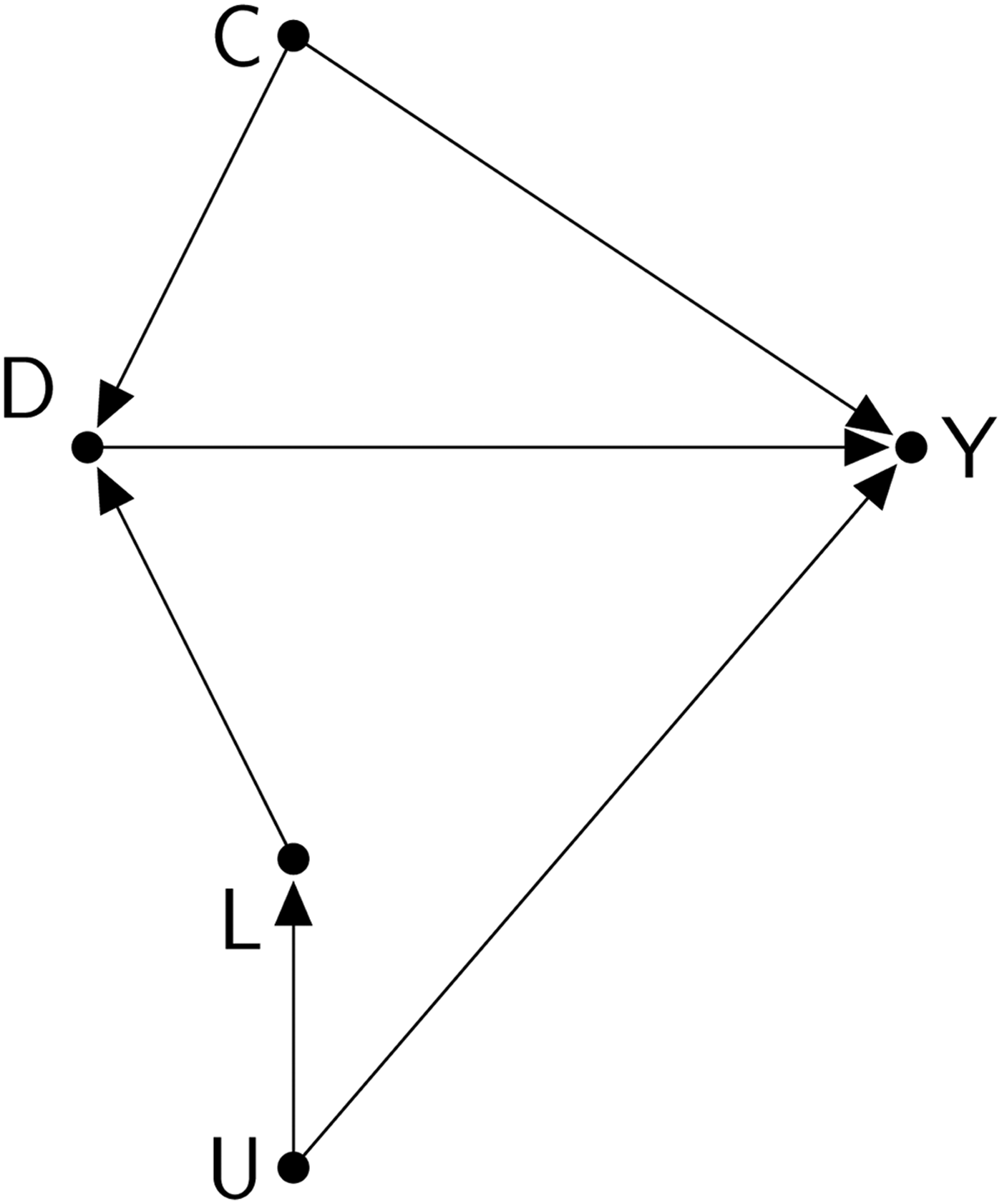
A DAG displays three types of causal effects: direct effects, total effects, and indirect effects. Consider the nodes C and Y in Figure 1. The direct effect of C on Y is indicated by a single arrow from C to Y. Indirect effects of C on Y are indicated by those directed paths that flow through one or more other nodes usually refered to as mediators. In Figure 1, C has a indirect effect on Y through D. The total effect of C on Y is comprised of all the causal paths that begin at C and end at Y. Next, we turn to identification. We only focus on the identification on total effects. See Imai et al. (Reference Imai, Keele, Tingley and Yamamoto2011), Acharya et al. (Reference Acharya, Blackwell and Sen2016), and Van der Weele (Reference Van der Weele2015) for more details on indirect and direct effects.
Identification in a DAG depends on the property of d-separation, which is used to determine whether two variables are causally connected or not. When two variables are d-separated in a DAG, they will be statistically independent, but if two variables are d-connected they will typically be statistically associated. Variables may be d-connected under three scenarios. First, they will be d-connected if one isa direct cause of another such as D → Y in Figure 1. Second two variables will be d-connected if they share a common cause that is not conditioned on. In Figure 1, L and Y are d-connected since they share the common cause U that is not conditioned on. Finally, two variables will be d-connected if a variable they both effect is conditioned on. In Figure 1, C and L are d-separated, but will be d-connected if one were to condition on D. Next, an indirect causal effect is a sequence of paths with all the paths pointing in the same direction. In Figure 1, the indirect effect of C on Y is given by: C → D → Y. Finally, a collider is a variable that is affected by two other variables; in Figure 1 D is a collider since paths from C and L collide into it. A collider is said to be activated if it has been conditioned on, and unactivated if not. Critically, dependence does not flow through a unactivated collider, but does flow through an activated collider. Thus if we condition on D, L and C will be dependent even though in the DAG they are independent. That is, if we condition on D, they will be d-connected.
With these principles, one can use the DAG for an identification analysis. First, the analyst draws the DAG. Next, the analyst must classify the variables in a DAG. Obviously, one variable must be classified as the outcome, and then one variable is classified as the treatment or intervention. An identification analysis under selection on observables will classify which of the other “independent” variables should be used as controls, and which should be ignored. The identification analysis is always done relative to which variables the investigator selected as the outcome and treatment.
Next, the analyst should ensure the DAG is complete. A DAG is complete if every common cause of any two variables on the graph is included. This includes unobserved common causes.Footnote 6 It is the assumption of the completeness that is often controversial in that other investigators can assert that some common cause has been left off and thus identification is no longer valid. Assuming a DAG is complete, however, is entirely consistent with the selection on observables assumption. Under selection on observables, the analyst asserts that he or she has the complete set of variables that predict whether units select in or out of treatment. The completeness of DAGs is observationally equivalent in that one assumes he or she has the complete set of variables that block all back-door paths between D and Y.
To use the DAG to identify the total effect of D on Y, we must first identify all the causal paths between D and Y. These are often called front-door paths, since they are causal paths that flow out of D. Next, we must block all confounding paths between D and Y. These paths are often called back-door paths since these are paths that point into D. If there are a set of observed variables W that block all back-door paths, then the set W satisfies the back-door criterion relative to the effect of D on Y. Finally, to satisfy the back-door criterion, W cannot contain any colliders that would unblock back-door paths and no element of W can be a descendent of D. If W does satisfy the back-door criterion, the causal effect is identifiable using the back-door adjustment formula. Under further functional form assumptions, one could estimate the causal effects of D on Y using methods like regression to control for W. Finally, the back-door criterion can be used to identify effects for sets of treatment variables where effects are interpreted as joint interventions. Effects of this type are known as causal interactions (Van der Weele, Reference Van der Weele2009). From our reading of the literature, observational studies of this type are relatively rare in the political science literature. In what follows, we focus on single interventions.
2.2. Graphs and causal interpretations
As we outlined above, statistical estimates of treatment effects can be given causal interpretations when the identification strategy implies that a treatment is independent of potential values of Y. A DAG is one method that investigators may use to clarify which variables have causal interpretations in statistical models. It is only identified effects that deserve causal interpretations after estimation occurs. Imagine the following research process to understand how this process might work. The analyst writes down a DAG. He or she uses it to derive which causal effects are identified. The analysts then proceeds to estimate a regression model. Keep in mind that we have defined the term regression broadly to include nonparametric methods. As such, we bracket functional form considerations. This is not to minimize the bias that can result from functional form misspecification. However, there are a wide variety of estimation methods available to avoid restrictive functional form assumptions. Instead we focus on the following question: which of the estimates in the regression model can be given a causal interpretation? The investigator can give causal interpretations to those estimates that were found to be identified in the DAG. The estimates for control variables are not given a causal interpretation, since they are not identified. Thus the DAG can perfectly clarify the form of interpretation for the many estimates produced by a regression model. Next, we turn to two stylized examples to demonstrate how DAGs clarify the causal interpretation of estimates from regression models.
3. Examples
Here we provide two examples to demonstrate that while some estimates in a regression merit a causal interpretation, many estimates do not. For both examples, we develop one possible DAG for a theoretical question. While we think these DAGs are fairly realistic interpretations of the literature, they are not meant to serve as theoretical statements on these questions. Instead they are stylized representations of these literatures, since our goals are methodological and not theoretical. The main purpose of these DAGs is to demonstrate how the interpretation of regression estimates depends directly on the assumed causal structure represented in the DAG. As such, we are assuming additionally that the use of a linear regression model to estimate the effects identified in the DAG is unproblematic. Finally, our examples do not include the use of data or the actual estimation of models. Our main point is about what an assumed causal structure implies about model estimates, and thus we need not estimate a model to understand those implications.
3.1. Example 1: effective number of parties
First, we develop an example drawn from the literature on comparative electoral systems. In comparative politics, a great deal of research has focused on identifying the factors that determine the number of parties that will compete in elections and the level of electoral support each will receive (jointly understood as the “effective number of parties” in the system). Since Duverger (Reference Duverger1959), comparativists have asked whether the structure of electoral systems causes the effective number of parties and posited various mechanisms that would suggest such a relationship. Most famously, Duverger argued that single member district systems encouraged bipartisan while proportional representation encouraged multiple parties. The most comprehensive updating of Duverger's logic is due to Cox (Reference Cox1997), who generalized the argument to the hypothesis that, under a wide variety of electoral systems, the maximum number of parties competing and receiving support in an electoral district should be the number of seats at stake plus 1. Other researchers have also theorized about these relationships and estimated empirical models intended to provide evidence about them (Powell, Reference Powell1982; Taagepera and Shugart, Reference Taagepera and Shugart1989; Ordeshook and Shvetsova, Reference Ordeshook and Shvetsova1994).
Figure 2 contains a DAG that represents a possible causal structure drawn from our reading of this literature for the effective number of parties in some legislative electoral district. We do not claim that this DAG fully represents any one scholar's theory or captures all the important debates in this literature. Indeed, for pedagogical clarity, we have left out several important ideas in this literature that a fuller treatment should include (e.g., the role of proximity between legislative and presidential elections). The variables that are included, however, capture some of the most important debates in the literature including not only district magnitude but the anti-productive impact of upper tier allocation formulas, societal cleavages, and the interaction between presidential and legislative party systems. We have also included an unmeasured common cause U of several variables, which one can think of as including unmeasured influences like partisan rhetorical strategies (e.g., Przeworski and Sprague (Reference Przeworski and Sprague1986)) that can both heighten or depress societal divisions—and so shape societal cleavages—while also conditioning support for current parties in both the legislative and presidential races. Finally, we must assume that this DAG is complete. That is, we have included every common cause of any two variables in the model. As we noted before, the assumption of completeness is our assertion that we have the complete set of variables that we need to adjust for. A typically controversial claim in many applications. For example, here we are assuming that Social Cleavages and Upper Tier Seat Allocation do not share any common causes. This is a strong assumption that must be defended. However, the DAG makes this assumption explicit in a way that is often unclear when investigators assert identification under selection on observables.
One possible DAG for the effective number of legislative parties. a Electoral rules for presidential elections.

We assume that the researcher is interested in estimating a single total causal effect (specifically, the effect of district magnitude on the effective number of parties) from a regression model that includes as controls for the other measured variables in the DAG (we consider a case in which a researcher wants to compare multiple causal effects in the next example). For this example, we consider only an additive specification (as used by several important studies) and ignore more complicated interactive specifications (e.g., Cox, Reference Cox1997, ch. 11). The question we ask then is what causal interpretation, if any, is justified for these control variables? First, we note that, given the DAG in Figure 2, the main causal effect of interest, the total effect of district magnitude on the effective number of legislative parties, can be identified by adjusting for observables. While there are many back-door paths between district magnitude and the expected number of legislative parties, each of these runs through at least one of the observable noncollider variables (Number of Social Cleavages or the Existence of Upper Tier Seat Allocation) and so can be blocked by including those variables as controls in a model. Likewise, there are no variables that mediate between district magnitude and the effective number of legislative parties and no collider variables introduced by conditioning on any of the observables. Thus, the total effect of district magnitude on the effective number of legislative parties can be nonparametrically identified by conditioning on the following variables: number of social cleavages, the number of presidential parties, and the existence of upper tiers observable. Suppose that we believe the DAG in Figure 2 holds, and we decide to use a linear empirical model (without interactions) to estimate the total effect of district magnitude on the effective number of parties. However, we include all the variables in the DAG in the model. Note this very simple specification is for illustrative purposes only. One could use a method like KRLS to produce a more flexible fit but also interpretable output for all the model parameters. As such, the analyst estimates the following model:

Next, using the information from the DAG, we review the causal interpretation of each of the estimated coefficients:
• β1 does not represent a total effect because it does not account for the indirect effect of upper tiers through legislative district magnitude.
• β2 represents the total effect of district magnitude on the effective number of legislative parties since this total causal effect is identified.
• β3 does not represent a causal effect, since the effect of social cleavages is unidentified due to unblocked back-door paths.
• β4 does not represent a causal effect, since the effect of electoral rules is unidentified due to unblocked back-door paths (and this variable is not even necessary to identify the main causal effect of interest and so could be dropped from the model).
• β5 does not represent a causal effect, since the effect of the effective number of presidential parties is unidentified due to unblocked back-door paths.
Thus, only one of the four coefficients in Equation 1 represents a total causal effect, that of district magnitude. In contrast, the total effect of upper tier allocation cannot be estimated from this regression model, given the causal structure in the DAG. The regression coefficient on the measure of upper tier allocation only represents a direct effect.Footnote 7 Further, no effects (either direct or total) of social cleavages or the effective number of presidential parties are identified. Therefore, in these cases, the estimated regression coefficients do not represent a causal quantity of any kind. While a measure of social cleavages is necessary to identify the effect of district magnitude on the effective number of legislative parties, its casual effect is not identified under this DAG. This demonstrates the hazards of attempting to interpret all the coefficients in a regression model. Unless one understands the causal structure, regression coefficients can represent any number of quantities.
It will strike some readers as absurd for us to say that β4 represents nothing since the effect of social cleavages on the effective number of legislative parties is unidentified. One might say: aren't regression coefficients always interpretable even when they don't represent causal effects? One might claim that β4 represents a conditional association but not a causal effect given the DAG in Figure 2. However, these are conditional associations given the control set in the DAG, as such, interpretation of unidentified conditional associations is not recommended. Thus while the number of social cleavages and the effective number of legislative parties may be (positively) correlated in this regression, one should not take this result as evidence that the number of social cleavages has any causal effect on the effective number of legislative parties.
In general, this leads to a broader point about estimated associations (as opposed to causal effects). In a given empirical literature, there are almost always some relationships for which estimated associations in different empirical models are unstable (i.e., when a given covariate, D, is included in different specifications for Y, the estimated association between D and Y is sometimes statistically significant and sometimes not and/or its sign changes frequently). It is easy to accept the conclusion that the estimated coefficients for these kinds of relationships are just associations that are likely spurious. It is more challenging, however, to accept this judgment for more stable associations—that is, a relationship between D and Y, that across many different empirical models, reliably produces statistically significant coefficients with the sign in the expected direction. Whether one can interpret such coefficients as causal depends on what causal structures one believes to be true, and there is no reason to assume that the stability of the estimated coefficients indicates, by itself, a causal effect. It is entirely possible that there area set of unobserved confounders that are themselves stable – thus producing a reliable estimated association in many different models and specifications.
Finally, we outline two specific structures in a DAG that lead to this lack of causal interpretability for a regression coefficient. Figure 3 contains two DAGs with the general structure that leads to this phenomenon. In both cases, L blocks a back-door path between D and Y, therefore we must condition on L to identify the effect of D on Y. However, in both cases, the effect of L is not identified, therefore it would be problematic to provide any interpretation for a regression coefficient for L when one is trying to estimate the effect of D on Y. Therefore, if one suspects one of these structures is in operation, one must take care in the interpretation of coefficients as casual effects.
DAG structures that lead to regression coefficients that cannot be interpreted as causal effects. In panel (a) L has no effect on Y and in panel (b) the confounder, L, has an effect on Y. In both cases, one must condition on L to identify the effect of D on Y, but the effect of L on Y is not identified. (a) One structure for confounding. (b) A second structure for confounding.

3.2. Example 2: vote choice in US elections
In the previous example, we considered the case in which an analyst specified a model with the goal of identifying a particular causal effect—the impact of democracy on conflict—and so chose a set of control variables considered sufficient to block all open back-door paths to identify that effect. As we saw, it is not always possible to give the estimated associations between these control variables and the outcome a causal interpretation. Another common situation, however, occurs when a researcher has several different causal hypotheses that he or she wishes to simultaneously examine (and adjudicate among) and so includes measured variables that capture these different hypotheses in a single regression model. Clearly, given the structure of such studies, the estimated coefficient on each variable requires a casual interpretation.
As an example, consider a researcher who has collected survey data on a set of variables capturing the generally accepted causes of vote choice and wants to estimate the relative importance of these drivers for the election at hand. A stylized, but eminently recognizable, selection of such covariates might include party identification, perceptions of economic performance, relative issue stances (perhaps aggregated into general left–right positions), and perceived candidate qualities, characteristics, or images. Each of these covariates comes from a well-developed theoretical literature, and we suspect that most electoral researchers would agree that these concepts often have causal effects on vote choice—recognizing, of course, that these effects may or may not be apparent in any given election. Clearly, the hypotheses that our electoral researcher wishes to test are causal and so the question is whether all four causal effects (party id, economic performance, candidate quality, and relative issue positions) can be tested in the kind of single equation empirical model usually used in such situations? Again, an appropriate DAG (or set of DAGs) can help answer this question.
Here, using a DAG, one can show which of the causal effects of interest are identified given the causal assumptions the investigator is willing to invoke. For example, the DAG in Figure 4 provides one plausible causal structure for vote choice with these variables and others as causes. Using the back-door criterion, we can determine that in this DAG three of the main causal effects are identified. Thus, we can identify the effects of candidate qualities, economic perceptions, and issue positions. It is worth repeating that these causal inferences are conditional on the assumed theoretical structure of the DAG. For example, in this DAG there is a single unobserved confounder affecting party identification and vote choice. This is a strong assumption, since one could, for example, imagine that there might be unobserved common causes between party identification and issue positions. If one articulated a different data generating process, one would draw different conclusions about what causal inferences are possible.
One possible DAG for a model of vote choice.

This pattern of identification stems from two sources. First, the DAG makes a set of exclusion restrictions sufficient to eliminate unblocked back-door paths between any of the variables of interest and the outcome. For example, the DAG implies there are no unmeasured variables that impact both a respondent's issue positions and her views of the economy. In a mature literature in which many of the most important confounders have been identified, this is perhaps a reasonable position to take—and is, at least implicitly, the position taken by many electoral researchers that estimate and interpret vote choice models. Note however that the effect of party identification on the vote is not identified in this DAG, since there is an unblocked back-door path—running through U—between it and vote choice. Here, U might represent early parental influences that condition both party id and vote choice.
Further, what is very clear from this DAG—and perhaps not otherwise—is that this happy situation of simultaneous identification of the causal effects for each causal hypotheses of interest (other than party id) depends almost entirely on the fact that in this theoretical specification, party id is a sort of “super-blocker” of back-door paths. By controlling for party id, one manages, in one stroke, to simultaneously block the back-door paths that would otherwise confound each of the three (nonparty id) variables of interest. A DAG of this type is consistent with the theoretical position that party id is the “unmoved-mover”—as many students of American electoral behavior do (e.g., Campbell et al., Reference Campbell, Converse, Miller and Donald1966; Green and Palmquist, Reference Green and Palmquist1994; Miller and Shanks, Reference Miller and Shanks1996; Green et al., Reference Green, Palmquist and Schickler2004). A different strand in the literature argues that short-term factors like issue positions (Carsey and Layman, Reference Carsey and Layman2006; Highton and Kam, Reference Highton and Kam2011), candidate characteristics (Page and Jones, Reference Page and Jones1979), and economic perceptions (Fiorina, Reference Fiorina1981; MacKuen et al., Reference MacKuen, Erikson and Stimson1989) can, at least under some conditions, move party id. A proponent of this theory would undoubtedly draw a different DAG. For our methodological purposes, we draw just a single DAG.
Next if we assumed that this data generating process is linear without any interactions, we might estimate the following regression model:

In this regression model, vote choice is a function of all the observed covariates in the DAG. Under standard advice about complete specifications, one would hesitate to leave any of these covariates out of the right-hand side of the model. Following the discussion above, the coefficients for economic perceptions, candidate qualities, and issues can be interpreted as estimates of the identified total effects, while the coefficient for party identification cannot be given a causal interpretation as any type of effect. In this regression model, party identification serves to block open back-door paths, but its coefficient, β1, cannot be given a causal interpretation since it causes the other covariates and shares an unmeasured set of causes with vote choice. Indeed, even if party id did not share common causes with vote choice, the fact that the regression specification conditions on the decedents of party id means this estimated association is not a total causal effect.Footnote 8 Under these conditions, the total effect of party id could be estimated in a bivariate regression of party id on vote choice. Likewise, based on the graph, the coefficient on the real economy, β6, is not a total effect, since the model conditions on decendents of this variable. Finally, the coefficient on demographics, β2, cannot be interpreted as a total causal effect in this model (since again the model conditions on its descendants) and neither does it represent a direct effect. However, its total effect can easily be estimated (given the DAG) with a bivariate regression of demographics on vote choice.
More generally, this example demonstrates that it is possible to conduct a test of rival hypotheses in a single regression model. That is, multiple estimates in a regression model may merit a casual interpretation. However, as we noted above, it is only through a causal identification analysis that one can separate which estimates are for causal effects and which are for associations. Casual graphs are one way for analysts to clearly demonstrate which estimates deserve causal interpretations. In general, we would also argue that analysts should take great care when giving causal interpretation to regression estimates. Moreover, additional care must be taken when more than one regression estimate is given a causal interpretation. While it is possible multiple causes are identified, we think that in general this will be a difficult enterprise. Only a well-grounded identification analysis can reveal which estimates merit a causal interpretation. Finally, we must emphasize that use of a DAG does not mean the causal effects are actually identified. That is, any causal interpretation given to a regression estimate based on a DAG assumes the DAG represents the true causal structure, which is an assumption that readers may question or accept. Our point is that once a DAG is presumed to be true, researchers may use it to clearly identify which estimates in a regression model merit a causal interpretation.
4. A brief literature review
One might accept the premise of our argument, but insist that empirical practice in the discipline has advanced beyond this issue. Perhaps, giving causal interpretations to multiple regression coefficients is a thing of the past. To that end, we selected an issue of the American Political Science Review for review—specifically, the first issue of 2017. This issue contained 13 research articles, and seven of these did not contain any empirical results. The remaining six articles all focused on making causal inferences using data, and they were all observational studies. Of these six articles, three focused on a single treatment effect and did not provide multiple causal interpretations (Gulzar and Pasquale, Reference Gulzar and Pasquale2017; Kim, Reference Kim2017; Klasnja and Titiunik, Reference Klasnja and Titiunik2017). The other three empirical investigations examined multiple causes absent clear identification arguments for each cause. Moreover, each gave causal interpretations to multiple regression coefficients (Gibler, Reference Gibler2017; Goren and Chapp, Reference Goren and Chapp2017; Touchton et al., Reference Touchton, Sugiyama and Wampler2017). While our review is certainly not systematic, it does show that in a very recent issue of the leading journal in political science this practice is common.
5. Conclusion
In this paper we attempt to explain how careful theoretical thinking about causal structures is necessary to answer a set of questions that have long troubled political scientists: how should multiple estimates from a regression model be interpreted when causal inference is the goal? We outlined that identification strategies are what give estimates causal interpretations. Thus each treatment of interest in a study will require a carefully articulated and defended identification strategy. Often it will not be practical to examine more than one causal effect at a time. Finally, we conclude with some guidelines. Researchers should minimally
• Carefully articulate an identification strategy. All causal analyses require one.
• Each treatment of interest requires a separate assessment of identification.
• Researchers should avoid providing any interpretation for estimates of control variables.
Acknowledgments
We would like to thank Judea Pearl, Alan Dafoe, Josh Kertzer, and seminar participants at Yale University and University of California, Davis for helpful comments.



